A Practical Guide to ROS 2 and Jetson for Humanoid Robotics
1. Humanoid Robotics Requirements and System Architecture
1.1 Define Humanoid Use Cases and Operational Constraints
A humanoid robot is not “a robot with legs.” It’s a system that must coordinate perception, balance, manipulation, and safety while operating under strict physical limits. Start by writing use cases in a way that forces clarity: what the robot must do, what it must not do, and what conditions must hold for success.
Identify Humanoid Use Cases That Fit the Hardware
Choose use cases that map cleanly to the robot’s capabilities. A good use case includes a primary task, supporting tasks, and measurable outcomes.
- Primary task: e.g., “Pick up an object from a table and place it into a bin.”
- Supporting tasks: e.g., “Maintain balance while reaching,” “Detect the object,” “Plan a collision-free path,” “Execute joint commands within limits.”
- Outcome: e.g., “Object ends inside the bin within 2 cm,” “No contact with prohibited zones,” “Robot returns to a stable stance after placement.”
A practical trick: write the use case twice—first as a human description, then as a checklist of required signals (pose, joint states, contact state, object pose). If you can’t list the signals, the use case is probably too vague.
Specify Operational Constraints That Prevent Surprise
Operational constraints are the rules the robot must obey even when everything else is going well. Treat them like engineering requirements, not preferences.
-
Environment constraints
- Lighting range for cameras (e.g., normal indoor lighting, not direct sunlight).
- Floor properties that affect traction and slip risk.
- Allowed obstacles and their minimum clearance.
-
Timing constraints
- Control loop frequency for balance and joint actuation.
- Maximum acceptable perception latency for tasks that require tracking.
- End-to-end action timing budgets, such as “reach and grasp within 3 seconds.”
-
Physical constraints
- Joint position, velocity, and torque limits.
- Maximum center-of-mass deviation before recovery is required.
- Reach envelope and self-collision boundaries.
-
Safety constraints
- Prohibited contact regions and emergency stop behavior.
- Maximum allowable force at the hands during interaction.
- Safe fallback posture when sensors degrade.
-
Reliability constraints
- What “success” means when perception is uncertain.
- How many retries are allowed before the robot must stop.
- Logging requirements for post-run diagnosis.
Turn Use Cases into Requirements
Convert each use case into a small set of requirements that can be tested. For example, for “pick and place,” define:
- Perception requirement: object pose must be published at a known rate with a defined frame.
- State requirement: robot base pose must be available to the controller with bounded error.
- Control requirement: joint commands must respect limits and produce stable stance transitions.
- Interaction requirement: grasp attempt must stop if contact force exceeds a threshold.
If you can’t attach a number or a pass/fail condition to a requirement, it will be hard to debug later.
Mind Map: Use Cases and Constraints
Example: From Task Description to Constraints
Use case: “Approach a person’s hand, grasp a lightweight object, and place it on a shelf at chest height.”
- Environment constraints: indoor lighting; shelf height within a known range; keep a minimum distance from the person’s torso.
- Timing constraints: approach motion must slow down when hand tracking confidence drops; grasp attempt must complete within a fixed window.
- Physical constraints: limit arm speed near the person; enforce joint torque caps during contact.
- Safety constraints: stop motion if the robot enters a forbidden zone; cap hand force during contact.
- Reliability constraints: if object pose is lost twice, retreat to a stable stance and wait.
This example shows why constraints belong early: they shape the controller behavior, the perception confidence handling, and the motion planning strategy.
Example: A Minimal Use Case Template
Use this template to keep each use case testable:
- Task:
- Start condition:
- End condition:
- Required sensors/signals:
- Frames and coordinate conventions:
- Timing budgets:
- Physical limits:
- Safety rules:
- Success criteria:
- Failure handling:
When you fill it in, you’ll naturally discover missing pieces like coordinate frames, contact sensing needs, or recovery behaviors. That’s the point: constraints turn vague ideas into buildable robot behavior.
1.2 Map Sensors Actuators and Compute Resources to Functional Blocks
A humanoid robot is easiest to build when you treat hardware as a set of functional blocks, not a pile of devices. The goal of this section is to map each sensor and actuator to the software responsibilities that consume or command it, and then assign compute resources to those responsibilities.
Start with Functional Blocks, Not Parts
Begin by listing the robot’s core runtime responsibilities. For a practical humanoid, a common set is:
- State estimation: turn raw sensor readings into a consistent robot state.
- Perception: detect and track objects, people, and surfaces in the robot’s view.
- Planning: decide where the robot should move next.
- Whole body control: convert plans into joint-level commands that respect constraints.
- Safety and diagnostics: detect faults, enforce limits, and keep the system recoverable.
- Communication and orchestration: move data between components at the right rates.
Now map hardware to these responsibilities. A sensor rarely belongs to only one block; for example, IMU data feeds both state estimation and safety checks.
Map Sensors to Consumers and Data Contracts
For each sensor, define:
- What it measures (units and reference frame)
- What it outputs (message type and fields)
- What consumes it (which functional blocks)
- How often it updates (expected rate)
- What quality looks like (latency tolerance, noise expectations)
A useful rule: if you cannot state the reference frame and units, you are not ready to integrate the sensor.
Example: IMU mapping
- State estimation consumes angular velocity and linear acceleration to update orientation and motion.
- Safety consumes angular velocity spikes to detect falls or impacts.
- Compute assignment: IMU processing is lightweight but time-critical, so it should run on a CPU core with predictable scheduling.
Example: Depth camera mapping
- Perception consumes depth images to build a local 3D representation.
- Planning consumes obstacle geometry derived from perception.
- Safety consumes near-field occupancy to prevent collisions.
- Compute assignment: depth preprocessing and inference are heavier, so they belong on a GPU-capable compute path.
Map Actuators to Command Interfaces and Control Loops
Actuators should be mapped to the control responsibilities that generate their commands. For each actuator group, define:
- Command type: position, velocity, effort/torque, or mixed
- Control loop ownership: which block closes the loop
- Limits: max speed, max torque, joint travel bounds
- Feedback: which sensors provide joint state
Example: Joint motors
- Whole body control owns the loop that outputs desired joint positions or torques.
- State estimation provides joint angles and velocities from encoders.
- Safety monitors limit violations and controller divergence.
If your actuator driver expects a different command type than your controller produces, insert a small “command adapter” block. This keeps the rest of the system honest and reduces hidden conversions.
Assign Compute Resources by Workload Shape
Compute mapping is about workload shape, not just raw speed.
- Time-critical, low-latency: sensor timestamping, state propagation, safety limit checks.
- Throughput-heavy: image preprocessing, feature extraction, depth filtering.
- Algorithmic, moderate latency: planning, kinematics, collision checking.
- Deterministic control: whole body control updates at a fixed cycle.
A practical Jetson-style split is:
- CPU: state estimation, controller logic, safety checks, orchestration.
- GPU: perception inference and image/depth preprocessing.
- Optional microcontroller: low-level motor drivers and fast fault handling.
Mind Map of the Mapping Process
Mind Map: Mapping Hardware to Functional Blocks
Integrated Example: From Sensors to Commands
Suppose you want the robot to take a step toward a visible target.
- Perception consumes RGB and depth to produce a target pose and nearby obstacles in the robot’s local frame.
- State estimation fuses IMU and joint encoders to maintain an accurate base pose and joint velocities.
- Planning uses the target pose and obstacle geometry to generate a short horizon trajectory.
- Whole body control converts the trajectory into joint commands while enforcing joint limits and balance constraints.
- Safety continuously checks for unexpected motion, excessive joint effort, and imminent collisions, then triggers a safe stop if needed.
The mapping step ensures each block knows exactly which hardware feeds it, what it must output, and what timing it must respect. When that is in place, integration becomes mostly wiring and verification rather than guesswork.
1.3 Choose ROS 2 Communication Patterns for Real Time Robot Behavior
Real-time robot behavior depends less on “fast computers” and more on choosing the right communication pattern for each job. In ROS 2, the main patterns are topics, services, and actions. The practical rule is simple: use topics for continuous streams, services for request-response work that must finish, and actions for long-running tasks that can be preempted.
Topics for Continuous State and Sensor Streams
Topics are the default choice when data changes over time: camera frames, IMU readings, joint states, planned trajectories, and controller commands. Topics fit real-time behavior because publishers and subscribers can run independently, and you can tune delivery behavior with Quality of Service (QoS).
A useful mental model is “producer-consumer with timing.” If the consumer is late, you usually want the newest data, not an old backlog. For that reason, many sensor pipelines use a QoS profile with a small history depth and a best-effort reliability setting. For control loops, you often prefer reliable delivery but still keep history small to avoid stale commands.
Example: a joint state pipeline.
- A hardware interface publishes
/joint_statesat 200 Hz. - A state estimation node subscribes and publishes
/robot_state. - A whole-body controller subscribes to
/robot_stateand publishes/joint_commands.
If the controller misses a cycle, it should use the most recent state it has, not wait for older messages. That is a QoS and scheduling decision, not a “hope for the best” decision.
Services for Synchronous Decisions
Services are for operations that behave like “do one thing and return a result.” They are appropriate for calibration triggers, mode switches, or queries that must be answered immediately by some component.
Services are not ideal for high-rate control because each request creates a tight coupling between caller and callee. In real-time systems, tight coupling can cause jitter: if the callee is busy, the caller stalls.
Example: a safety node that answers “Is it safe to start walking?”
- The controller sends a service request to
/safety/check_start. - The safety node checks current contact sensors and joint limits.
- The service returns a boolean plus a reason code.
The controller can then transition states without continuously polling. That reduces unnecessary traffic and keeps the decision path explicit.
Actions for Long-Running Tasks with Preemption
Actions are for goals that take time: grasping, walking, searching, or multi-step manipulation. Actions add feedback and allow cancellation, which is crucial for humanoid behavior where the robot must react to new information.
An action server accepts a goal and streams feedback. The client can cancel when conditions change, such as a new obstacle detected or a balance controller requesting an abort.
Example: a “reach and grasp” action.
- Client sends goal: target pose and grasp type.
- Server plans and executes in phases.
- Feedback includes current stage and estimated completion time.
- If perception updates the target, the client cancels the current goal and sends a new one.
This pattern keeps the control logic clean: continuous control stays in topics, while the high-level task lifecycle uses actions.
Mind Map: Communication Pattern Selection
Putting It Together: A Humanoid Behavior Split
A reliable architecture separates responsibilities:
- Use topics for the control loop inputs and outputs:
/joint_states,/tf,/robot_state,/wrench,/joint_commands. - Use services for discrete transitions:
/set_stance,/enable_balance_controller,/safety/check_start. - Use actions for task-level behaviors:
/walk_to,/reach_grasp,/get_up.
This separation prevents the most common timing problem: a controller waiting on a service while it should be computing the next command. Instead, the controller reads the latest topic data every cycle, while higher-level nodes manage goals and state transitions.
Example: End-to-End Message Flow for Walking
- Topics:
/imuand/joint_statesupdate state estimation./robot_statefeeds balance control./cmd_velor/footstep_targetsfeeds the walking controller.
- Service:
/safety/check_startis called once when a walk request arrives.
- Action:
/walk_toruns the walking task.- Feedback reports progress and current phase.
- Cancellation stops the task when balance constraints are violated.
When each pattern is used for its natural job, the system becomes easier to reason about under timing pressure. The robot still has to be fast, but now it also has predictable behavior when messages arrive late, goals change, or safety conditions flip.
1.4 Establish Data Flows for Perception Planning Control and State Estimation
A humanoid robot behaves like a chain of cause and effect: sensors produce measurements, state estimation turns them into a consistent world model, perception produces task-relevant observations, planning turns goals into trajectories, and control turns trajectories into actuator commands. Data flows are the wiring that makes this chain reliable under real timing constraints.
Foundational Data Contracts
Start by defining what each stage outputs and what it consumes. Use message contracts that are explicit about frame, timestamp, and units.
- Measurements: raw sensor outputs such as camera detections, IMU samples, joint encoders.
- State: a consistent estimate of robot pose, velocities, and optionally contact state.
- Perception Outputs: task-level observations such as “hand is near cup” or “support foot is stable.”
- Plans: time-parameterized trajectories or discrete motion primitives.
- Commands: actuator-level setpoints with safety limits.
A practical rule: every message that crosses a stage boundary must include a timestamp and a frame identifier (or an explicit statement that it is frame-free). If you skip this, debugging becomes guesswork.
System Timing and Synchronization
ROS 2 nodes run concurrently, so you need a timing strategy.
- Choose a reference clock: typically the ROS time source aligned with your sensor timestamps.
- Stamp early: stamp messages as close to the sensor acquisition as possible.
- Handle latency: perception and estimation may run slower than sensors, so downstream consumers must tolerate stale data.
- Use consistent update rates: for example, state estimation at 100 Hz, planning at 10 Hz, control at 200 Hz.
If you use a fixed control loop, treat planning and perception as asynchronous inputs that the controller samples at each tick.
Core Flow: From Sensors to State Estimation
State estimation is the glue that makes perception and planning agree on “where the robot is.” A typical flow looks like this:
- Joint encoders and IMU feed an estimator.
- The estimator publishes robot state in a known frame tree.
- TF transforms provide the mapping between frames.
When you publish state, include both pose and velocity if your controller needs them. If you only publish pose, you will end up estimating velocity again inside control, often with different assumptions.
Perception Flow: From Images to Task Observations
Perception should produce outputs that planning can use without reinterpreting raw pixels.
- Camera node publishes images and/or detection results.
- A perception node converts detections into geometry using known camera intrinsics and TF transforms.
- The perception node publishes observations in a stable frame, such as
base_linkormap.
A simple contract for perception outputs is: what it is, where it is, how confident you are, and when it was observed. Confidence can be a scalar or a boolean gate, but it must be consistent across the pipeline.
Planning Flow: From Goals to Trajectories
Planning consumes state and perception outputs.
- Inputs: current robot state, target pose or object pose, and constraints.
- Outputs: a trajectory with time stamps or a method to compute desired setpoints at time
t.
To keep the pipeline coherent, planning should reference the same frame tree used by state estimation. If planning outputs are in odom but control expects base_link, you will get “it moves but not where you think” bugs.
Control Flow: From Trajectories to Actuation
Control consumes plans and produces actuator commands.
- The controller runs at a fixed rate.
- Each tick, it samples the latest plan and computes desired joint positions, velocities, or torques.
- Safety logic clamps commands based on joint limits, velocity limits, and estimated contact state.
A useful pattern is to separate trajectory following from safety gating. That way, you can test the follower with a simulated actuator interface before adding safety constraints.
Mind Map: Integrated Data Flow
Example: Pick-and-Place Data Flow with Clear Contracts
Assume a “reach to grasp” behavior.
- Perception publishes
object_poseinbase_linkwith timestampt_obj. - State estimation publishes
robot_stateinodomand TF transforms. - Planning runs at 10 Hz, reads the latest
robot_stateandobject_pose, and outputs a trajectory inodomwith time stamps. - Control runs at 200 Hz, samples the trajectory at the controller tick time, and outputs joint setpoints.
If t_obj is older than a threshold, planning can either reject the observation or replan using the last valid pose. The key is that the decision is explicit and based on timestamps, not on “it seems fine.”
Example: Minimal Topic Set for Coherent Wiring
    flowchart LR
  A[Camera + Detections] --> B[Perception Node]
  C[IMU + Encoders] --> D[State Estimation Node]
  E[TF Transforms] --> B
  E --> D
  B --> F[Perception Observations]
  D --> G[Robot State]
  F --> H[Planner]
  G --> H
  H --> I[Trajectory]
  G --> J[Controller]
  I --> J
  J --> K[Joint Commands]
This wiring keeps each stage’s responsibility narrow: perception produces task geometry, estimation produces consistent robot state, planning produces time-based motion, and control produces safe actuator commands.
1.5 Set Up a Reproducible Development Workflow for Hardware and Software
Reproducibility means you can take a fresh machine, run the same commands, and get the same behavior: builds succeed, nodes start, and sensor-to-actuator pipelines behave as expected. For humanoid robotics, that includes both software determinism and hardware determinism, because a “working” setup that depends on one developer’s laptop is not a setup.
Define What “Reproducible” Means for Your Robot
Start by writing a short checklist of outcomes you will reproduce. For example: “A clean checkout builds all packages,” “a single launch brings up perception and state estimation,” and “hardware interfaces publish joint states at the expected rate.” Then decide which parts must match exactly (ROS 2 distribution, message definitions, controller parameters) and which can vary within limits (log file names, absolute paths, machine hostnames).
A practical trick: treat each outcome as a testable acceptance criterion. If you cannot measure it, you cannot reproduce it.
Pin the Software Stack and Make It Portable
Reproducibility starts with pinning versions. Use a single source of truth for:
- ROS 2 distribution and build tool versions
- OS packages that affect builds (compiler, dependencies)
- Python dependencies used by scripts
- Message/service/interface packages that other nodes rely on
Containerization helps because it freezes the environment. The goal is not “containers everywhere,” but “one known-good runtime.” Keep the container image build steps explicit and deterministic, and ensure the workspace is mounted read-only when running tests.
Standardize the Workspace Layout and Build Commands
Use a consistent workspace structure so paths and package discovery behave the same way. A common pattern is:
src/contains packagesbuild/,install/,log/are generated artifacts- launch and config files live inside packages so they travel with the code
Then standardize commands: one script for “setup,” one for “build,” one for “test,” and one for “run.” This removes the “I ran it with a different flag” problem.
Example workflow commands (adapt names to your repo):
# setup
./scripts/setup.sh

# build
./scripts/build.sh

# tests
./scripts/test.sh

# Run a Known Demo
./scripts/run_demo.sh
Capture Hardware Configuration as Data, Not Memory
Humanoid robots fail in boring ways: wrong serial device, swapped USB ports, mismatched joint limits, or a controller tuned for a different actuator. Put hardware configuration into versioned files:
- device mappings (e.g.,
/dev/ttyUSB*rules by serial number) - calibration parameters (encoder offsets, IMU orientation)
- controller gains and safety limits
- URDF/Xacro parameters that define link lengths and joint axes
Use a single “hardware profile” selector so the same launch file can run against different robots without editing code.
Make Launch Behavior Deterministic
Launch reproducibility is about ordering, parameters, and timing. Ensure:
- nodes receive the same parameter sets every time
- TF frames are published consistently
- simulation and hardware modes differ only where necessary
- startup waits for required topics or services when appropriate
A simple rule: if a node depends on another node’s data, encode that dependency in the launch logic rather than relying on “it usually starts fast enough.”
Add Verification Steps That Catch Drift Early
Verification should run quickly and fail loudly. Include:
- build checks (linting, unit tests)
- runtime smoke tests (topic presence, message schema compatibility)
- timing checks (expected publish rates for joint states and sensor streams)
- safety checks (controller limits loaded and within bounds)
Keep logs structured so you can compare runs. For example, record controller parameter hashes and calibration file versions at startup.
Use a Mind Map to Keep the Workflow Coherent
Mind Map: Reproducible Development Workflow
Integrated Example: From Clean Checkout to Hardware Smoke Test
Assume you have a humanoid_bringup package with a launch file and a hardware_profiles/ directory.
- Clean checkout and setup:
./scripts/setup.shinstalls pinned dependencies and builds the workspace.
- Select a hardware profile:
run_demo.sh --profile lab_robot_aloads calibration and controller limits from versioned files.
- Start bringup deterministically:
- launch injects parameters, publishes TF frames, and starts state estimation before controllers begin commanding.
- Run smoke verification:
test.shchecks that joint states publish at the expected rate and that the controller reports loaded limits.
If any step fails, the failure message should point to the exact layer: environment, build, configuration, or runtime dependency. That’s what makes the workflow reproducible instead of merely repeatable.
2. Installing ROS 2 and Setting Up a Jetson Development Environment
2.1 Select A ROS 2 Distribution And Align It With Jetson Software Versions
Choosing the right ROS 2 distribution for Jetson is mostly about compatibility. The goal is simple: make sure your ROS 2 packages, the underlying Ubuntu base, and the Jetson software stack agree on versions so you spend time building robot behavior instead of chasing dependency errors.
Start with the Jetson Baseline
First identify what Jetson software you are actually running. On most systems this means the JetPack version and the Ubuntu release it includes. ROS 2 distributions are built against specific Ubuntu versions, and Jetson images often pin you to a particular Ubuntu release.
A practical workflow:
- Check your Jetson OS release (Ubuntu version).
- Check your JetPack version.
- Pick a ROS 2 distribution that targets that Ubuntu release.
- Confirm you can install the ROS 2 packages you need using the same package manager strategy you plan to use (binary packages vs source builds).
If you skip step 1, you can end up with a ROS 2 install that compiles but fails at runtime due to mismatched system libraries.
Match Ubuntu Compatibility Before Anything Else
ROS 2 distributions are tied to Ubuntu releases. For example, if your Jetson runs Ubuntu 20.04, you should focus on ROS 2 distributions that support 20.04. If your Jetson runs Ubuntu 22.04, you should focus on ROS 2 distributions that support 22.04.
When you align Ubuntu first, the rest becomes easier:
- System dependencies like DDS implementations and networking libraries are consistent.
- Message generation tools and build tooling behave predictably.
- You reduce the chance of “works on my machine” when you later move from development to deployment.
Decide Between Binary Install and Source Build
Binary installs are faster and usually sufficient for typical robot stacks. Source builds are useful when you need a package version that is not available as binaries for your exact Ubuntu/ROS combination.
A rule of thumb:
- Use binary ROS 2 when your required packages exist for your chosen distribution.
- Use source builds when you must patch a dependency, add a missing package, or build a custom message/service interface.
If you choose source builds, align your build toolchain with the Jetson OS. That means using the same compiler version family expected by the Ubuntu release and keeping your workspace clean.
Keep DDS and Networking in Mind
ROS 2 uses DDS for discovery and data exchange. Different DDS vendors can behave differently under constrained networks and different multicast settings.
On Jetson, you typically want to ensure:
- Your ROS 2 middleware choice is consistent across all machines in the system.
- Your network interfaces are stable (avoid switching Wi-Fi/Ethernet mid-session).
- Your firewall rules do not block discovery traffic.
This matters because a “correct” ROS 2 install can still appear broken if discovery never completes.
Use a Simple Version Alignment Checklist
Before installing ROS 2, write down the versions you will align. This prevents accidental drift when you later rebuild.
Mind Map: Version Alignment Checklist
Example: Aligning a Jetson with ROS 2 On Ubuntu 20.04
Assume your Jetson runs Ubuntu 20.04. You select a ROS 2 distribution that supports 20.04 and install it using the standard ROS 2 apt approach. Then you verify that core tools work before adding robot-specific packages.
A minimal validation sequence:
- Confirm ROS 2 environment sourcing works.
- Confirm
ros2command availability. - Confirm a basic publisher/subscriber example can exchange messages.
If those steps succeed, you can proceed to your robot stack with much less risk.
Example: When You Must Use Source Build
Suppose your robot requires a package version that is not available as binaries for your exact ROS 2 distribution. You can still keep the system stable by:
- Installing the ROS 2 base using binaries.
- Building only the missing packages from source in a separate workspace.
- Keeping the workspace isolated so you do not accidentally override system packages.
This approach limits the surface area where version mismatches can occur.
Common Pitfalls to Avoid
- Mixing ROS 2 packages built for different Ubuntu releases.
- Installing ROS 2 base binaries and then rebuilding core ROS 2 components without a clear reason.
- Changing DDS or network settings between nodes during debugging.
A small amount of upfront alignment saves hours later, especially when you start integrating perception and control where timing and message flow matter.
Quick Decision Summary
Pick the ROS 2 distribution that matches your Jetson’s Ubuntu release, choose binary install when possible, and validate basic ROS 2 communication before adding custom robot packages. That sequence keeps your foundation solid and your humanoid stack easier to reason about.
2.2 Install ROS 2 on Jetson and Configure Networking for Development
A solid ROS 2 setup on Jetson starts with two goals: (1) the right software versions, and (2) networking that behaves predictably when multiple machines and devices are involved. This section walks through both in a systematic order, from baseline checks to practical multi-device workflows.
Confirm Jetson Baseline and ROS 2 Compatibility
Before installing anything, verify the Jetson OS and architecture so you don’t end up debugging package mismatches. Check that you are on an ARM64 system, confirm the Ubuntu release (or the Jetson Linux base), and note whether you’re using a desktop environment or a minimal install. ROS 2 packages expect a consistent set of system libraries, so keep the OS stable during the install.
A practical habit: record the output of your system checks in a short note file on the Jetson. When something breaks later, you’ll know whether the issue is code or environment.
Install ROS 2 on Jetson with a Reproducible Approach
Use the ROS 2 installation method that matches your target ROS 2 distribution and Jetson OS. The key is to install ROS 2 in a way that can be repeated on a fresh device.
- Update package lists and upgrade system packages.
- Install ROS 2 using the official repository method for your ROS 2 distribution.
- Source the ROS 2 environment in your shell and verify the core tools.
- Run a minimal test to confirm nodes can start and communicate locally.
Example: after installation, open a new terminal and run the ROS 2 CLI to list available topics. If the CLI works but no topics appear, that’s normal until you start nodes.
# Terminal 1
source /opt/ros/<ros_distro>/setup.bash
ros2 topic list

# Terminal 2
source /opt/ros/<ros_distro>/setup.bash
ros2 run demo_nodes_cpp talker
If you see the talker output in Terminal 2, you’ve confirmed the ROS 2 runtime is functional.
Configure Networking for Reliable Discovery
ROS 2 discovery relies on DDS, which uses network interfaces and multicast. On Jetson, the most common failure mode is “it works on one machine but not the other,” caused by interface selection, firewall rules, or mismatched network settings.
Start by identifying the network interface you will use for development, such as eth0 for wired or wlan0 for Wi‑Fi. Use a static IP for the development network when possible, because DHCP changes can silently break discovery.
Mind map of the networking checklist:
Mind Map: Jetson Networking for ROS 2
Set Environment Variables for Deterministic DDS Behavior
When you have multiple interfaces or containers, DDS may bind to the wrong one. To reduce surprises, set environment variables that constrain DDS to the intended interface and, when needed, specify discovery behavior.
A common approach is to set the ROS 2 domain ID so all machines in the same project share the same discovery scope. Pick a domain ID and keep it consistent across Jetson and your workstation.
Example: set the domain ID and ensure both machines use it.
# On Jetson and on the Workstation
export ROS_DOMAIN_ID=42
Then verify discovery by running a node on one machine and checking topics from the other.
Validate Local and Cross-Machine Communication
Validation should be incremental: first confirm ROS 2 works locally, then confirm discovery across devices.
- Local test on Jetson: start a talker and confirm it appears in
ros2 topic list. - Cross-machine test: start talker on Jetson, run
ros2 topic echoon the workstation. - If discovery fails: check IP reachability (ping), confirm both machines are on the same subnet, and re-check firewall settings.
Example workflow:
# Jetson
source /opt/ros/<ros_distro>/setup.bash
export ROS_DOMAIN_ID=42
ros2 run demo_nodes_cpp talker
# Workstation
source /opt/ros/<ros_distro>/setup.bash
export ROS_DOMAIN_ID=42
ros2 topic list
ros2 topic echo /chatter
If /chatter appears and ros2 topic echo prints messages, networking is correctly configured.
Handle Common Jetson Networking Pitfalls
If you can’t see topics across machines, the issue is usually one of these:
- Wrong interface: DDS may bind to a different NIC than the one you’re using.
- Firewall blocking multicast or UDP traffic: discovery can fail even when TCP tools like SSH work.
- Domain mismatch: different
ROS_DOMAIN_IDvalues isolate discovery. - Subnet mismatch: machines on different networks won’t share multicast discovery.
A quick sanity check is to confirm both machines report the same ROS_DOMAIN_ID and can reach each other at the IP level.
Create a Development-Ready Shell Setup
To avoid forgetting environment variables, add them to your shell startup so every terminal session is consistent. This includes sourcing ROS 2 and setting the domain ID.
Example snippet for ~/.bashrc:
source /opt/ros/<ros_distro>/setup.bash
export ROS_DOMAIN_ID=42
After updating, open a new terminal and rerun the cross-machine test. Consistency beats memory, especially when you’re juggling multiple nodes and devices.
2.3 Build and Test Core ROS 2 Packages From Source When Needed
Building from source is the “I need exactly this version” option. You use it when a prebuilt package is missing, too old, or built with different options than your Jetson setup. The goal is simple: produce a workspace that builds cleanly, runs predictably, and fails in understandable ways.
When Source Builds Are Worth It
Start by listing the reason you need source builds:
- You need a specific commit or patch for a driver or message definition.
- You need to compile with flags that match your Jetson environment.
- You want to test changes to a core package without waiting for binary releases.
A practical rule: if you can describe the mismatch in one sentence, source builds are usually justified.
Workspace Foundations That Prevent Pain
Use a consistent workspace layout so builds and tests behave the same across machines.
- Keep your ROS 2 installation separate from your workspace.
- Use a single workspace for the packages you actively modify.
- Prefer building only what you changed plus its dependencies.
A typical workflow is:
- Create or reuse a workspace.
- Add the target packages to the workspace source tree.
- Resolve dependencies.
- Build with colcon.
- Run tests and basic runtime checks.
Mind Map: Source Build Workflow
Dependency Resolution Without Guesswork
Before compiling, resolve dependencies deterministically. The most common failure mode is “it builds on my machine” caused by missing system packages or mismatched versions.
A systematic approach:
- Identify the packages you will build.
- Run dependency resolution for those packages.
- Re-check that the dependency list matches the ROS 2 distribution you installed.
If dependency resolution fails, treat it as a data problem: inspect the missing package name and version, then install the exact system dependency that satisfies it.
Building with Colcon Like You Mean It
Use colcon to build only what you need. This reduces build time and makes failures easier to interpret.
Example: build a single package and its dependencies.
# From the Workspace Root
source /opt/ros/<distro>/setup.bash
colcon build --packages-up-to <package_name>
Example: rebuild only a set of packages after changes.
source /opt/ros/<distro>/setup.bash
colcon build --packages-select <pkg_a> <pkg_b>
When a build fails, read the first error, not the last. Later errors often cascade from the first missing header, type mismatch, or CMake option.
Testing Strategy That Matches Robot Reality
Tests come in layers. Unit tests confirm logic; integration tests confirm message flow; runtime checks confirm the system starts and publishes what you expect.
A practical testing sequence:
- Run package tests for the packages you built.
- Run any available launch-based tests.
- Start a minimal node graph and verify key topics.
Example: run tests for selected packages.
source /opt/ros/<distro>/setup.bash
colcon test --packages-select <package_name>
colcon test-result --verbose
If tests are missing, don’t treat that as a dead end. Replace them with a minimal runtime verification: start the node, check that it publishes expected topics, and confirm parameters load correctly.
Example: Building a Custom Message Package Safely
Suppose you added a new message type used by multiple nodes. Build and test in a way that catches downstream breakage.
- Build the message package.
- Build the nodes that depend on it.
- Run tests or at least start those nodes and verify they can subscribe.
Example: build up to a dependent package.
source /opt/ros/<distro>/setup.bash
colcon build --packages-up-to <dependent_node_package>
Then run a minimal launch or node start and confirm the subscriber receives messages without type errors.
Debugging Build and Test Failures Systematically
When something breaks, classify the failure:
- CMake configuration errors usually mean missing dependencies or incompatible build options.
- Compile errors usually mean API changes or mismatched message definitions.
- Test failures usually mean assumptions about timing, parameters, or environment.
For timing-related test failures, reduce variables: run tests with the same environment variables and parameters you used during manual runtime checks.
Integrated Checklist for Source Builds
- Reason for source build is documented in one sentence.
- Workspace structure is consistent.
- Dependencies are resolved before compilation.
- Build uses package-scoped colcon commands.
- Tests run for built packages, followed by runtime verification.
- Failures are handled by first-error analysis and environment consistency.
A good source build ends with confidence you can reproduce: the same commands, the same workspace, and the same node behavior. That’s the whole point—no mystery, just controlled engineering.
2.4 Configure User Permissions and Device Access for Cameras and Sensors
Humanoid robots tend to fail in boring ways: a camera node starts, then silently can’t open /dev/video0; a sensor driver runs as root in development but fails in production; or a container can see the device but not the permissions. This section makes device access predictable by treating permissions as part of the system design, not an afterthought.
Foundational Concepts for Device Access
Linux device access is usually controlled by three layers:
- Device node permissions: e.g.,
/dev/video0has an owner, group, and mode bits. - User and group membership: the process runs as a user that must match the device node’s group.
- Security boundaries: systemd service settings, udev rules, and container device mappings.
ROS 2 adds one more practical layer: nodes often run under launch-managed processes, so the effective user/group must be correct at runtime, not just in your shell.
Step 1: Identify Devices and Their Current Permissions
Start by listing device nodes and their metadata:
ls -l /dev/video*ls -l /dev/ttyUSB* /dev/ttyACM*for serial sensorsudevadm info -q property -n /dev/video0to see identifying properties
Record the device path, group name, and mode. If you see crw-rw---- with a group like video, that’s your target group for the process.
Step 2: Create Stable Device Ownership with Udev Rules
Device numbers can change across reboots, so permissions should be attached to identity, not to /dev/video0 specifically. Use udev rules to set group and mode based on stable attributes (vendor/product IDs, serial numbers, or physical port identifiers).
A typical rule sets the group to video and ensures read/write access for that group. Keep the rule minimal: set what you need, avoid broad permissions like 0666 unless you have a controlled environment.
Step 3: Align ROS 2 Runtime User and Group
If you run ROS 2 nodes as your login user, ensure that user is in the relevant groups:
videofor V4L2 camerasdialoutfor serial devices- any vendor-specific group used by your udev rules
Then verify the effective permissions from the same context ROS 2 uses. For example, if you start via systemd or a launch script that uses sudo, the effective user changes and permissions may break.
Step 4: Configure Systemd Services Without Permission Surprises
When ROS 2 is launched as a service, set the user explicitly in the service file. Also ensure the service has access to the device nodes by relying on the udev rules you created.
Example systemd service settings:
[Service]
User=robot
Group=robot
SupplementaryGroups=video,dialout
DeviceAllow=/dev/video0 rw
DeviceAllow=/dev/ttyUSB0 rw
Use SupplementaryGroups rather than changing the main group, because it keeps the service’s primary identity stable while granting device-specific access.
Step 5: Handle Containers with Device Mapping
If you run ROS 2 nodes inside a container, two things must be true:
- The container must be started with access to the device nodes.
- The process inside the container must run with a user/group that matches the device node permissions.
A common approach is to map /dev/video* and /dev/ttyUSB* into the container and run with the same numeric UID/GID as the host user that owns the udev-assigned group.
Mind Map: Permissions and Device Access Flow
Example: Fixing a Camera That Won’t Start
Suppose a camera node logs an error like “cannot open device” while your shell can access it.
- Compare contexts: run the node the same way systemd/launch runs it.
- Check device permissions:
ls -l /dev/video0and note the group. - Confirm the service user is in that group:
SupplementaryGroups=video. - If the group changes after reboot, add a udev rule so the camera always lands in the same group.
- If using a container, ensure the container is started with
--device=/dev/video0(or a broader mapping like/dev/video*if appropriate).
Example: Serial Sensor Access for a Humanoid IMU
For a serial IMU on /dev/ttyUSB0:
- Ensure udev assigns the device to
dialout(or your custom group). - Add the ROS 2 runtime user to
dialout. - If the driver runs under systemd, set
SupplementaryGroups=dialout. - Validate by checking that the node can open the port and that it can read expected bytes (not just that the port exists).
Practical Validation Checklist
Before moving on, confirm these points in order:
- Device nodes have the intended group and mode.
- The ROS 2 runtime user has matching supplementary groups.
- systemd services specify the correct user and supplementary groups.
- Containers map the device nodes and run with compatible UID/GID.
- A simple “open and read” test succeeds for each sensor type.
Once these are consistent, permission issues stop being mysterious and start being mechanical—exactly what you want when the robot is standing still and you’re trying to make it move.
2.5 Validate The Environment With Deterministic Build And Runtime Checks
A Jetson + ROS 2 setup is deterministic only if you can reproduce both the build outputs and the runtime behavior. This section gives you a practical checklist that starts with foundational reproducibility and ends with runtime verification that catches the annoying failures: missing devices, wrong clocks, mismatched message types, and silent performance regressions.
Lock Down the Build Inputs
Determinism starts before you compile. First, record the exact ROS 2 distribution and Jetson software baseline you are targeting. Then ensure your workspace uses a consistent dependency resolution strategy.
Best practice: keep one “source of truth” for environment variables.
- Put ROS 2 and workspace paths in a single shell script you can run on demand.
- Avoid relying on interactive shell history or IDE-specific environment settings.
Easy example: create env-setup.sh that exports ROS_DOMAIN_ID, RMW_IMPLEMENTATION, and your workspace path, then source it before every build and run.
Use Reproducible Workspace Builds
A clean build is a sanity check, not a ritual. Build deterministically by controlling the workspace state and build options.
Best practice: build from a known state.
- Use a fresh
build/andinstall/directory when validating. - Keep compiler flags consistent across machines.
Easy example: run a clean build once, then compare artifact timestamps and package summaries. If you see unexpected rebuilds, trace which package or dependency changed.
Verify Package Graph and Interfaces
Runtime failures often come from interface mismatches that still compile. Confirm that the package graph and generated interfaces match what your nodes expect.
Best practice: check the resolved package list and message/service/action types.
- Ensure every node you run is using the intended package version from your workspace install.
- Confirm that message definitions are consistent across the nodes that communicate.
Easy example: after building, run a node that publishes a known message and another that subscribes, then verify the subscriber receives the expected fields and frame IDs.
Validate Runtime Environment Before Launch
Before launching a full humanoid stack, validate the runtime environment in small steps.
Best practice: test the “plumbing” first.
- Confirm network reachability if you use multiple machines.
- Confirm camera and sensor device visibility.
- Confirm time sources and clock behavior.
Easy example: run a minimal ROS 2 node that prints the current ROS time and the system time. If they disagree in a way that breaks your assumptions, fix the clock configuration before you debug perception or control.
Deterministic Runtime Checks with Observability
Now you verify behavior, not just availability. Deterministic runtime checks focus on repeatable measurements.
Best practice: define pass/fail criteria for each subsystem.
- For perception: message rate, end-to-end latency, and dropped frames.
- For state estimation: transform availability and transform age.
- For control: command update frequency and saturation events.
Easy example: run your perception pipeline twice with the same inputs and compare metrics. If latency varies wildly, you likely have CPU contention, inconsistent QoS, or blocking callbacks.
Mind Map: Deterministic Build and Runtime Checks
Example: A Two-Stage Validation Workflow
Stage 1 checks build and interfaces.
- Source your environment script.
- Clean build the workspace.
- Run a small publisher/subscriber pair using the exact message types your real nodes will use.
- Confirm transforms or frame IDs are consistent with your URDF.
Stage 2 checks runtime behavior.
- Launch only the sensor driver and a lightweight consumer.
- Measure message rate and verify no unexpected drops.
- Add the next component (e.g., perception) and repeat the measurement.
- Add state estimation and confirm transform availability within expected time bounds.
If any stage fails, you stop there. That keeps the failure local instead of turning it into a full-stack mystery.
Example: Runtime Checklist for Common Humanoid Pitfalls
- Clock mismatch: ROS time vs system time causes stale transforms.
- QoS mismatch: sensor messages arrive late or not at all.
- Frame ID drift: transforms exist but don’t connect the expected tree.
- Device permissions: cameras or IMUs are “present” but not readable.
- Callback blocking: one slow callback reduces update frequency.
Use the checklist to decide what to fix first. Start with time, then QoS, then frames, then devices, then performance. That order prevents you from chasing symptoms caused by earlier configuration issues.
3. ROS 2 Core Concepts for Robot Software Engineering
3.1 Understand Nodes Topics Services and Actions in ROS 2
ROS 2 is built from a few core building blocks that map cleanly to how robots actually behave: components that run (nodes), messages that flow (topics), request-response interactions (services), and longer-running tasks with feedback and cancellation (actions). Once you can predict how these pieces interact, most robot software design decisions become straightforward.
Nodes: The Running Components
A node is a process (or part of a process) that performs computation and communication. In practice, you’ll create nodes for things like:
- A camera driver that publishes images.
- A perception node that subscribes to images and publishes detections.
- A controller node that subscribes to state and publishes joint commands.
Nodes communicate without direct references to each other. Instead, they meet through ROS 2 interfaces (topics, services, actions). This separation is what makes systems easier to test and swap.
Topics: Continuous Streams of Data
A topic is a named channel for one-way message flow. Publishers send; subscribers receive. Topics fit naturally for:
- Sensor streams (images, IMU, joint states)
- State estimates and transforms
- Logging or monitoring signals
A useful mental model: topics are for “keep talking.” If you stop publishing, subscribers simply stop receiving new data.
Example: Joint State Publishing and Consumption
- The hardware interface publishes
sensor_msgs/msg/JointState. - A visualization node subscribes and renders the robot.
- A controller node subscribes and computes commands.
# Terminal A: publish (conceptual)
ros2 topic echo /joint_states

# Terminal B: subscribe (conceptual)
ros2 topic list | grep joint
Services: One-Off Requests with Replies
A service is a request-response interaction. A client sends a request; a server returns a response. Services fit when you need a single answer, such as:
- “Set a parameter” style commands
- “Get current status”
- “Compute something once”
A useful mental model: services are for “ask and wait.” The client typically blocks until it receives a response (or times out).
Example: Triggering a Calibration Routine
- A calibration manager node offers a service like
std_srvs/srv/Trigger. - An operator UI calls the service.
- The server runs calibration steps and returns success plus a message.
# List Services
ros2 service list

# Call a Trigger Service (conceptual)
ros2 service call /calibrate std_srvs/srv/Trigger "{}"
Actions: Long Tasks with Feedback and Cancellation
Actions handle operations that take time and may need monitoring or interruption. An action includes:
- Goal request
- Feedback messages during execution
- Result when finished
- Cancellation support
Actions fit for:
- Moving a limb to a pose
- Navigating to a waypoint
- Whole-body motions that can be preempted
A useful mental model: actions are for “do work over time, keep me informed, and let me stop you.”
Example: Move Arm With Preemption
- A planner node sends an action goal to a motion executor.
- The executor publishes feedback like current progress or tracking error.
- If a new goal arrives, the client cancels the old one and sends the new goal.
# Inspect Available Actions
ros2 action list

# View Action Details (conceptual)
ros2 action info /move_arm
Choosing the Right Interface
The choice is mostly about interaction shape:
- Topic: continuous data flow, no built-in reply.
- Service: single request, single response.
- Action: multi-step task, feedback, cancellation.
When designing humanoid behaviors, this mapping prevents common mistakes:
- Don’t use a topic for “start and confirm” workflows; you’ll end up inventing acknowledgements.
- Don’t use a service for motions that take seconds; you’ll block and lose the ability to cancel cleanly.
- Don’t use an action for high-rate sensor streams; feedback becomes noisy and expensive.
Mind Map: Nodes Topics Services Actions
Putting It Together in a Humanoid Pipeline
Consider a simple reach behavior:
- A perception node publishes target pose on a topic.
- A behavior coordinator sends an action goal to the whole-body motion executor.
- The executor streams feedback (e.g., tracking error) via the action.
- If the target changes, the coordinator cancels the current goal and sends a new one.
- A service can be used for a one-time “enable/disable balancing mode” command.
This structure keeps responsibilities clean: topics move data, services handle quick interactions, and actions manage time and control flow. Once you can sketch this interaction graph, implementing the actual ROS 2 nodes becomes mostly wiring and message contracts.
3.2 Use Quality of Service Profiles for Sensor Streams and Control Loops
Quality of Service (QoS) in ROS 2 is how you state your communication preferences: how reliable delivery should be, how long data is kept, and what happens when messages arrive faster than they can be processed. For humanoids, the key is to treat sensor streams and control loops differently. Sensors usually tolerate occasional loss but not stale data; control loops usually tolerate small delays but must not silently drop critical commands.
Start with the QoS Building Blocks
Think of QoS as four knobs that you set consistently across publishers and subscribers.
- Reliability:
RELIABLEaims for delivery;BEST_EFFORTallows drops to keep latency low. - Durability:
VOLATILEmeans only new subscribers get future messages;TRANSIENT_LOCALlets late joiners receive the last message. - History and Depth:
KEEP_LASTwith a depth controls how many samples are queued;KEEP_ALLcan grow unbounded. - Deadline and Lifespan: these express timing expectations; they help detect when data is too late or should be considered expired.
A practical rule: for high-rate sensors (cameras, IMUs), prefer low-latency settings with bounded queues; for low-rate state or command topics, prefer reliability and bounded queues.
Mind Map: QoS Choices for Humanoid Systems
Apply QoS to Sensor Streams
For sensor streams, you want subscribers to process the newest data, not a backlog. Use KEEP_LAST with a small depth so the queue acts like a “latest sample” buffer. For example, an IMU at 200 Hz feeding state estimation should not accumulate 100 old samples if the estimator hiccups.
A common setup for IMU-like data:
- Reliability:
BEST_EFFORT - Durability:
VOLATILE - History:
KEEP_LAST, depth5 - Lifespan: slightly above the expected processing interval
For cameras, the same logic applies, but the depth often stays at 1 or 2 because image processing is expensive and you want the newest frame. If you use RELIABLE for images, you can end up waiting for retransmissions and increasing end-to-end latency.
Apply QoS to Control Loops
Control loops are sensitive to missing commands and inconsistent timing. If a controller receives no command updates for a moment, it should not keep acting as if nothing happened. QoS can help by making the system fail loudly instead of quietly.
For command topics (joint targets, gait phase updates, mode changes), prefer:
- Reliability:
RELIABLE - Durability:
VOLATILE - History:
KEEP_LAST, depth1 - Deadline: set to the expected command period
Depth 1 is intentional: it ensures the controller always sees the most recent command, while reliability ensures that the latest command is not lost without the publisher knowing.
Keep QoS Consistent Across the Graph
QoS mismatches can cause subscriptions to connect but not exchange data as you expect. A reliable way to avoid surprises is to define QoS profiles in one place and reuse them across nodes. In ROS 2, you typically create a QoS object and pass it to publishers and subscriptions.
Example: IMU subscriber QoS tuned for freshness.
#include "rclcpp/rclcpp.hpp"
using rclcpp::QoS;

QoS imu_qos(rclcpp::KeepLast(5));
imu_qos.best_effort();
imu_qos.durability_volatile();
// Lifespan and deadline are optional but useful when supported.
// imu_qos.lifespan(rclcpp::Duration(10ms));
// imu_qos.deadline(rclcpp::Duration(5ms));
Example: Joint command publisher QoS tuned for correctness.
#include "rclcpp/rclcpp.hpp"
using rclcpp::QoS;

QoS cmd_qos(rclcpp::KeepLast(1));
cmd_qos.reliable();
cmd_qos.durability_volatile();
// cmd_qos.deadline(rclcpp::Duration(10ms));
Validate with Observable Behavior
QoS settings should be validated by what you can observe: latency, queueing, and whether timing expectations are violated. When you set a deadline or lifespan, you gain a mechanism to detect when the system is not meeting its own assumptions.
A simple validation workflow:
- Start with conservative depths (1–5) to prevent backlog.
- Run the pipeline and watch for missed deadlines or expired samples.
- If estimation lags, reduce depth or switch reliability to
BEST_EFFORTfor that sensor. - If control commands appear to “skip,” increase reliability or verify the publisher period matches the deadline.
Common Humanoid Pitfalls
- Using
RELIABLEeverywhere: it can turn transient overload into persistent latency. - Using large queue depths: it hides timing problems by letting old data arrive late.
- Ignoring timing policies: without deadline/lifespan, stale data can look valid and cause subtle instability.
- Changing QoS between nodes: keep profiles consistent so the behavior is predictable.
When you treat QoS as part of the control design rather than a networking afterthought, your humanoid stack becomes easier to reason about: sensors stay fresh, controllers stay responsive, and failures show up as measurable events instead of mysterious behavior.
3.3 Manage Parameters and Configuration for Repeatable Robot Behavior
Repeatable robot behavior starts with repeatable inputs. In ROS 2, parameters and configuration files are the knobs that turn “works on my machine” into “works on the robot.” The goal is not to cram everything into parameters, but to draw clear boundaries: what must be tuned per robot, what must be tuned per environment, and what must stay fixed to preserve safety and correctness.
Foundational Model of Configuration
Treat configuration as three layers.
- Build-time defaults: constants baked into code or URDF that rarely change.
- Deploy-time parameters: values loaded at startup, such as topic names, frame IDs, controller gains, and thresholds.
- Runtime adjustments: changes made while running, typically via parameter services, used sparingly for debugging or controlled tuning.
A practical rule: if changing a value can invalidate assumptions in other components, prefer deploy-time parameters and restart the affected nodes.
Parameter Design That Prevents Surprises
Use a consistent naming scheme and keep parameter types explicit. For example, prefer string for frame IDs, double for numeric thresholds, and bool for feature toggles. Group related parameters under a namespace-like prefix, such as perception.* or control.*, so logs and parameter listings remain readable.
Also decide who owns each parameter. If multiple nodes depend on the same value (like base_frame), define it once in a launch file and pass it to each node rather than letting each node guess.
Example: A Minimal Parameter Set for Repeatable Behavior
Imagine a humanoid demo where perception publishes detected objects and a controller decides whether to approach. The behavior depends on a few parameters:
perception.confidence_thresholdcontrols filtering.perception.target_classselects which detections matter.control.approach_distance_msets the stopping distance.control.max_velocity_mpscaps motion.
When these are set consistently, the same scenario produces comparable trajectories.
Launch-Time Configuration with Clear Ownership
In ROS 2, launch files are where you connect ownership to values. A launch file can declare parameters once and feed them to nodes. This reduces drift between nodes and makes it obvious what changed between runs.
from launch import LaunchDescription
from launch_ros.actions import Node

def generate_launch_description():
    return LaunchDescription([
        Node(
            package='humanoid_perception',
            executable='detector_node',
            name='detector',
            parameters=[{
                'perception.confidence_threshold': 0.65,
                'perception.target_class': 'cup',
                'use_sim_time': False,
            }],
        ),
        Node(
            package='humanoid_control',
            executable='approach_node',
            name='approach',
            parameters=[{
                'control.approach_distance_m': 0.35,
                'control.max_velocity_mps': 0.25,
                'base_frame': 'base_link',
            }],
        ),
    ])
This pattern makes the “run recipe” explicit: the parameters are visible in one place, and the nodes receive the same values every time.
Parameter Files for Robot-Specific Deployments
For a real robot, you often want a per-robot file that captures calibration and hardware-specific settings. Keep the file small and focused. For example, store:
- frame IDs and sensor mounting offsets
- controller gains that depend on actuator characteristics
- safety limits that must match the hardware
Then keep scenario-specific values in the launch file or a separate scenario file. This separation prevents accidental mixing of calibration and scenario tuning.
Runtime Parameter Changes Without Breaking Assumptions
Runtime updates are useful for debugging, but they can also create inconsistent internal state. When a parameter affects timing, coordinate frames, or controller structure, treat it as “restart required.” When it only affects a threshold or a filter, runtime updates are usually safe.
A disciplined approach:
- Log parameter changes with timestamps.
- Validate ranges before applying changes.
- If a change affects multiple nodes, update them together via the same operator action or script.
Validation and Guardrails
Repeatability improves when invalid configurations fail fast. Add checks at node startup:
- Ensure thresholds are within expected ranges.
- Ensure frame IDs are non-empty.
- Ensure numeric limits are consistent (e.g., max velocity is positive).
Also, make sure your node reports the effective parameter values on startup. When something goes wrong, you want to compare “effective parameters” rather than guessing what was intended.
Mind Map: Parameter Management for Repeatable Behavior
Case Example: Two Runs, One Outcome
Run A and Run B differ only in perception.confidence_threshold. With the same launch recipe otherwise, you can attribute behavior changes to that single parameter. If the robot approaches too early in Run B, you adjust the threshold and re-run. If the behavior changes unpredictably, the first suspect is configuration drift: nodes receiving different values, missing parameters, or frame IDs that differ between runs.
The practical win is simple: parameters become a controlled interface between your intent and the robot’s behavior, and the robot stops treating each run like a surprise quiz.
3.4 Implement Time Synchronization and Clock Handling for Robotics
Robots rarely fail because “time is hard.” They fail because different parts of the system disagree about what time it is, or because they treat timestamps as if they were interchangeable. In ROS 2, good clock handling means you can answer three questions reliably: What clock produced this timestamp? When did the event actually occur relative to that clock? How do you compare timestamps across nodes without guessing.
Foundational Clocks and Why They Matter
ROS 2 supports multiple time sources. The most important distinction is between system time (wall-clock time) and steady time (monotonic time that never goes backward). For robotics, steady time is usually the safer choice for measuring durations and ordering events, because it won’t jump when the system clock is corrected.
A practical rule: use steady time for timeouts, latency measurements, and “how long since X.” Use system time only when you must align with external references or human-readable schedules.
Time Domains in ROS 2
Each node can operate with a configured clock type. When you publish messages, the header timestamp is meaningful only within the same time domain. If one node uses system time and another uses steady time, comparing timestamps becomes meaningless even if both are “valid numbers.”
To keep things coherent, decide early: either standardize on steady time across your robot stack, or explicitly document where system time is required. Then enforce it in launch files and node configuration so you don’t end up debugging “negative latencies” that are really clock mismatches.
Timestamping at the Right Moment
Timestamping is not just “set header.stamp.” The timestamp should reflect when the measurement was taken, not when the message was processed. For example, a camera driver should stamp at capture time if it can. If it stamps at publish time, you must treat the timestamp as “time at handoff,” and compensate for transport and buffering.
A simple sanity check: if your perception pipeline reports consistent delays, but control uses those timestamps to predict motion, you’ll see systematic tracking errors. The fix is either better capture-time stamping or a consistent latency model that matches how timestamps are produced.
Synchronizing Sensor Streams
Time synchronization has two layers: within a sensor and across sensors.
Within a sensor, you want stable timing between frames and consistent metadata. Across sensors, you want to align measurements to a common reference so fusion doesn’t mix “now” from one stream with “then” from another.
In practice, you can implement approximate synchronization by buffering messages and pairing them by timestamp. The key is to define the tolerance window based on your worst-case jitter. If your IMU arrives with occasional bursts, a too-tight window causes dropped pairs; a too-loose window causes stale fusion.
Handling Latency and Jitter in Message Pipelines
Even with correct timestamps, pipelines introduce delay. A robust approach is to compute and log age at the consumer: age = now - msg.header.stamp. When age grows unexpectedly, you know the pipeline is falling behind or timestamps are not what you think.
Use age metrics to tune queue sizes, executor behavior, and callback scheduling. A queue that is too small drops data; one that is too large increases age and makes “latest” less meaningful.
Example: Consumer-Side Age Logging
# ROS 2 Python Example: Log Message Age Using the Node Clock
from rclpy.node import Node
from rclpy.time import Time
from sensor_msgs.msg import Imu

class ImuAging(Node):
    def __init__(self):
        super().__init__('imu_aging')
        self.sub = self.create_subscription(Imu, '/imu', self.cb, 10)

    def cb(self, msg: Imu):
        now = self.get_clock().now()
        stamp = Time.from_msg(msg.header.stamp)
        age = (now - stamp).nanoseconds / 1e6
        self.get_logger().info(f'IMU age_ms={age:.1f}')
This example assumes the publisher and subscriber share the same clock type. If they don’t, age will look wrong immediately, which is exactly what you want during integration.
Mind Map: Time Synchronization and Clock Handling
Advanced Details That Prevent Subtle Bugs
-
Use consistent frame semantics with time. If you transform sensor data using TF, ensure the transform lookup time matches the measurement time, not the current time. Otherwise, you effectively apply the wrong pose to the measurement.
-
Be explicit about time in transforms and interpolation. When you interpolate transforms, the interpolation time should be derived from the message timestamp. If you interpolate at “now,” you create a hidden prediction step.
-
Treat clock jumps as an error condition. If you must use system time, monitor for discontinuities. A single jump can reorder events and break filters that assume monotonic time.
-
Keep timeouts tied to steady time. Control loops and watchdogs should not depend on wall-clock time. If the system clock changes, your watchdog should still behave predictably.
Example: Correct Transform Lookup Timing
When you process a sensor message, use its timestamp for transform lookup so the pose matches the measurement moment.
# Pseudocode-style ROS 2 TF2 usage
# lookup_transform(target, source, msg.header.stamp)
# Then Apply Transform to the Measurement
This pattern is simple, but it eliminates a common class of “it works in simulation but not on hardware” issues caused by mismatched timing between sensor data and pose transforms.
3.5 Organize Workspaces with Packages Launch Files and Build Tooling
A ROS 2 workspace is more than a folder tree; it’s a contract between how you build, how you run, and how you debug. Good organization makes common tasks predictable: adding a package, running a single component, reproducing a build, and tracing where a message is produced.
Workspace Layout That Scales
Start with a single top-level workspace folder, typically named humanoid_ws. Inside it, keep only what belongs to the build: src for packages and optional install, build, and log directories created by the build tool.
Use a consistent naming scheme for packages:
humanoid_descriptionfor URDF/Xacro and related assetshumanoid_bringupfor launch files and system-level orchestrationhumanoid_perceptionfor vision nodes and message definitionshumanoid_controlfor controllers, interfaces, and action servers
This separation prevents a common failure mode: launch logic creeping into library code, or message definitions being scattered across unrelated packages.
Packages as Boundaries
Treat each package as a boundary with a clear purpose. A practical rule: if two parts of the system change independently, they should likely live in different packages.
Within a package, keep these roles distinct:
include/for headers (for C++ libraries)src/for executables and node implementationsconfig/for YAML parameterslaunch/for package-local launch filestest/for tests
When you define messages or services, place them in a dedicated package (for example, humanoid_interfaces). That keeps interface changes from forcing rebuilds of unrelated nodes.
Launch Files as Composition
Launch files should describe how to assemble the system, not how to implement it. A clean pattern is:
- Package-local launch files for a single subsystem (e.g., perception)
- A top-level bringup launch that composes subsystems
Keep launch files small by using arguments and including other launch files. For example, a bringup launch can accept use_sim_time, robot_model, and perception_mode, then pass those into subsystem launches.
Build Tooling That Stays Reproducible
Use colcon to build and test. The key is to build only what you need while keeping dependencies correct.
A typical workflow:
- Build everything once after major changes
- Rebuild only affected packages during iteration
- Always source the workspace
installsetup script before running
Example commands:
mkdir -p humanoid_ws/src
cd humanoid_ws
colcon build --symlink-install
source install/setup.bash
When you add a new package, build it immediately to catch missing dependencies early. If you use symlinks, you can iterate on code without constantly copying artifacts.
Mind Map: Organization Decisions
Example: A Minimal Bringup Structure
Imagine you want to start perception and state estimation together. Keep the perception node in humanoid_perception, and keep the system wiring in humanoid_bringup.
-
humanoid_perception/launch/perception.launch.py- starts camera driver and a detector node
- loads
config/perception.yaml
-
humanoid_bringup/launch/bringup.launch.py- includes
perception.launch.py - includes
estimation.launch.py - sets shared arguments like
use_sim_time
- includes
This structure makes it easy to run perception alone during debugging, while still allowing the full system to start with one command.
Practical Rules That Prevent Pain
- Keep interfaces in one place so message changes don’t ripple unpredictably.
- Keep launch logic in bringup packages so node code stays testable.
- Keep parameter files close to the package that owns the parameters.
- Build early and often after adding packages to surface dependency issues immediately.
When these rules are followed, the workspace becomes a reliable tool: you can add capabilities without breaking existing workflows, and you can reproduce a run by reusing the same launch arguments and parameter files.
4. Building a Humanoid State Estimation Stack with ROS 2
4.1 Model Robot Frames and Coordinate Transforms with TF2
Humanoid robots quickly become a coordinate-management problem: every sensor reading, joint state, and planned motion lives in some frame. TF2 is ROS 2’s way to keep those frames connected with time-stamped transforms, so your perception, estimation, and control code can agree on “where” things are.
Core Frames and Why They Matter
Start by naming frames with intent. A good frame set separates:
- Fixed world frames: e.g.,
mapfor global localization,odomfor drift-prone motion integration. - Robot base frames: e.g.,
base_linkat the robot’s center of mass reference. - Sensor frames: e.g.,
camera_link,imu_link. - Actuated link frames: e.g.,
left_hip_pitch_link,right_knee_pitch_link.
A practical rule: if a transform is purely geometric and never changes, publish it as static. If it changes with motion, publish it dynamically.
Transform Direction and Conventions
TF2 transforms are directional: T(A->B) answers “how to transform a point expressed in frame A into frame B.” In code, this often appears as lookup_transform(target_frame, source_frame, time).
To avoid silent mistakes, decide early:
- Use consistent axis conventions in URDF.
- Keep
base_linkas the anchor for most robot-centric computations. - Treat
map,odom, andbase_linkas a chain, not a jumble.
Building the Frame Tree with URDF
URDF defines the kinematic tree using link and joint. TF2 can mirror this tree, but only if you publish transforms that match the URDF joint origins and axes.
For a humanoid, you typically have:
- A root link (often
base_link). - A chain of joints from torso to each leg and arm.
- Sensor mounts as fixed joints off relevant links.
When you validate URDF, check that every joint has:
- A parent and child link.
- A correct origin (translation and rotation).
- A correct axis for revolute/prismatic joints.
Publishing Transforms with TF2
TF2 expects transforms to be published with timestamps. For a moving robot, transforms should be available at the same time as the sensor data you want to transform.
Common publishing pattern:
- Robot state publisher publishes transforms derived from joint states.
- Static transform publisher publishes fixed transforms like camera mounting.
If your IMU reports orientation in imu_link, you still need the geometric transform from imu_link to base_link so you can express IMU-derived quantities in the robot frame.
Mind Map: Frame Design and TF2 Workflow
Example: Transforming a Camera Detection into the Robot Base
Assume your vision system outputs a point in camera_link at time t. You want it in base_link.
- Ensure
camera_linkis connected tobase_linkvia a fixed transform. - Ensure the transform tree is being published.
- At runtime, request the transform at the detection timestamp.
# Pseudocode for Transforming a Point Using TF2
# target_frame: base_link
# Source_frame: Camera_link
# time: detection_time

transform = tf_buffer.lookup_transform(
    target_frame='base_link',
    source_frame='camera_link',
    time=detection_time
)

point_in_source = [x, y, z, 1.0]
T = transform_to_matrix(transform)  # 4x4 homogeneous
point_in_target = T @ point_in_source
If you use “latest” transforms instead of the detection timestamp, you may introduce small but annoying spatial errors, especially when the robot is moving.
Example: Debugging a Wrong Transform Direction
A classic failure looks like the robot thinks an object is behind it when it is in front. Often the transform direction is flipped.
- If you requested
lookup_transform('camera_link', 'base_link', t)but then applied it as if it werebase_link <- camera_link, your point will land in the wrong place. - Fix by consistently treating
target_frameas the frame you want the output expressed in.
Advanced Details That Prevent Headaches
Time synchronization: TF2 stores transforms over time. If your sensor timestamp is outside the buffer window, lookups fail. Align clocks and ensure your TF publisher rates cover the sensor rate.
Frame naming consistency: pick one naming style and stick to it. Mixing baseLink and base_link is the kind of bug that wastes an afternoon.
Chain length and performance: long chains are fine, but keep them intentional. If you can publish a direct static transform for a tool frame, do it.
Validation loop: visualize frames, then test with one known point. For instance, mount a checkerboard or marker at a fixed location and confirm that transforming its pose into base_link matches the expected geometry.
When frames are modeled cleanly and transforms are published with correct timestamps and directions, TF2 becomes boring—in the best way. Your robot code stops arguing about where things are, and you can focus on the actual task.
4.2 Fuse IMU and Joint States into a Consistent Robot State Representation
A humanoid needs a single, coherent “state” that other modules can trust: perception can reason about where things are, planners can predict motion, and controllers can command joints without fighting stale estimates. Fusion is the process of combining IMU orientation and joint encoders into one consistent pose and velocity estimate in the robot’s chosen frames.
Core Goal and Frame Discipline
Start by fixing the frame story. Pick a base frame (often base_link) and define how it relates to the world frame (often odom or map). IMU provides orientation relative to its own mounting frame (imu_link). Joint encoders provide positions and velocities relative to mechanical joints.
The consistency rule is simple: every published state must be expressible as transforms between frames and must agree with the kinematic model. If your TF tree says the base is at one orientation but your controller assumes another, you get oscillations that look like “tuning problems” but are actually bookkeeping problems.
What Each Sensor Contributes
IMU typically contributes:
- Orientation (roll/pitch/yaw or quaternion) at high rate.
- Angular velocity, useful for short-term motion.
- Linear acceleration, useful for gravity-aware tilt and sometimes velocity integration.
Joint states contribute:
- Kinematic pose of limbs and the base motion induced by leg/hip joints.
- Joint velocities that help estimate base velocity through the robot model.
A practical fusion approach is to use IMU for attitude (especially roll and pitch) and use joint-based kinematics for the rest, while keeping yaw consistent with your chosen reference.
Mind Map: the Fusion Pipeline
Step 1: Calibrate the IMU Mounting Transform
Your IMU is not mounted perfectly aligned with base_link. Create a fixed transform T_base_imu that maps IMU measurements into the base frame. A common workflow is:
- Keep the robot still.
- Measure the IMU orientation.
- Determine the rotation that makes the IMU’s gravity direction align with the base frame’s expected gravity direction.
Even a small mounting error shows up as a persistent tilt in the fused state. That tilt then leaks into foot contact logic and whole-body control.
Step 2: Time Synchronize and Resample
Fusion fails when timestamps don’t line up. Ensure IMU and joint states are time-aligned:
- Use the message header stamps.
- Resample to a common rate (often IMU rate) using the latest joint state for each IMU timestamp.
- If your joint states arrive slower, interpolate joint positions for smoother kinematics.
A good sanity check is to log the time difference between the IMU stamp and the joint stamp used for each update. If it drifts, you’ll see it as “mysterious lag” in the base orientation.
Step 3: Estimate Attitude with Gravity-Aware Roll and Pitch
Roll and pitch are strongly observable from gravity when the robot is not accelerating violently. Use IMU orientation directly for roll/pitch, but verify gravity alignment:
- Compute the gravity direction implied by the fused orientation.
- Compare it to the measured acceleration direction after removing bias.
If the robot is accelerating, gravity-based tilt can momentarily be wrong. In that case, rely more on gyro integration for short windows and blend back when acceleration stabilizes.
Step 4: Handle Yaw Without Fighting the Robot Model
Yaw is weaker in IMU alone because gravity doesn’t constrain it. Joint kinematics can help, but only if you have a reference for heading (for example, odometry from leg motion or an external yaw reference). A robust pattern is:
- Use IMU for roll/pitch.
- Use a yaw source that matches your TF world definition.
- Blend yaw slowly to avoid jumps when the yaw reference updates.
Step 5: Fuse Velocities and Publish a Consistent State
Once you have attitude, compute base twist consistently:
- Use gyro angular velocity for rotational velocity in
base_link. - Use joint velocities with the robot model to estimate translational velocity.
- If you integrate acceleration, do it in a gravity-compensated manner and keep bias under control.
Publish outputs so downstream nodes don’t need to guess:
- Publish TF
odom -> base_link(ormap -> base_link) using the fused pose. - Publish a state message that includes pose and twist with clear frame IDs.
- Keep debug topics for residuals, such as gravity alignment error and yaw discrepancy.
Example: Minimal Fusion Logic for Humanoid Base Attitude
Given:
- T_base_imu (fixed)
- q_imu(t) (IMU orientation in imu_link)
- q_yaw_ref(t) (yaw from your chosen reference)
Compute:
- q_base_from_imu = q(T_base_imu) * q_imu(t)
- Extract roll/pitch from q_base_from_imu
- Build q_fused = combine(roll_pitch_from(q_base_from_imu), yaw_from(q_yaw_ref))
- Publish TF using q_fused
- Use gyro ω_imu transformed to base_link for angular velocity
Validation Checklist That Catches Real Bugs
- TF consistency:
base_linkorientation in TF matches the fused quaternion used for control. - Gravity alignment: When standing still, roll/pitch residual stays near zero.
- Motion sanity: During slow walking, yaw changes smoothly without sudden discontinuities.
- Residual monitoring: Track the difference between predicted and measured gravity direction and angular rates.
A consistent state representation is less about fancy math and more about disciplined frames, careful timing, and fusion outputs that every module can interpret the same way.
4.3 Integrate Wheel or Leg Odometry with Sensor Inputs
Odometry gives you motion between time steps, but it drifts. Sensor inputs—IMU, joint encoders, contacts, and sometimes vision—provide corrections and constraints. Integration is about choosing what to trust at each moment and expressing that trust consistently in ROS 2.
Foundations: What Odometry Can and Cannot Do
Wheel odometry estimates planar motion from wheel speeds and geometry. Leg odometry estimates body motion from foot contacts, joint angles, and kinematics. Both share two limitations: (1) systematic errors from calibration and slip, and (2) unmodeled dynamics like impacts or uneven ground. The fix is not “more sensors”; it is a consistent state representation and a fusion method that respects timing.
A practical state for humanoids is usually a pose plus velocity in a chosen frame, plus sensor biases if you use an IMU. In ROS 2, you typically publish:
nav_msgs/Odometryfor the fused estimate or intermediate odometrysensor_msgs/Imufor raw IMUsensor_msgs/JointStatefor encoderstf2transforms for frame relationships
Mind Map: Integration Flow and Responsibilities
Step 1: Make Time and Frames Boring
Before fusion, ensure every message has a meaningful timestamp and a clear frame relationship. For example, wheel odometry might integrate in odom and output base_link pose. The IMU might be mounted with a fixed transform from imu_link to base_link. In ROS 2, you can keep the transform static and let the fusion node operate in one consistent frame.
A common mistake is mixing “measurement time” with “publish time.” If your wheel driver timestamps at receipt but your fusion uses sensor timestamps, you will see jitter in the fused pose even when the robot is still.
Step 2: Compute Odometry Increments with Uncertainty
Odometry integration should output both an estimate and a covariance (or at least a confidence score mapped to covariance). For wheels, slip increases uncertainty; for legs, missed contacts or foot scuffing increases uncertainty.
For wheel odometry, you can compute incremental motion from wheel angular velocities and wheel radius, then propagate covariance based on a slip model. For leg odometry, you can treat stance phases as constraints: when a foot is in contact, its position relative to the ground is more reliable than when it is swinging.
Even a simple approach helps: during stance, reduce covariance; during swing, increase it. This makes the fusion behave sensibly without requiring perfect modeling.
Step 3: Fuse with IMU and Constraints
A robust pattern is predict-correct:
- Predict: use IMU angular velocity to update orientation and use odometry for velocity/translation increments.
- Correct: use constraints from contacts (leg odometry) or occasional external pose (vision) to reduce drift.
If you already have a dedicated fusion package, the key is to feed it consistent inputs: correct covariances, correct frames, and measurements that match the expected message types.
For leg odometry, contact constraints are especially important. When both feet are in stance, you can constrain roll and pitch more tightly. When only one foot is in stance, yaw and translation along the support polygon are constrained differently.
Step 4: Use Gating to Prevent Bad Measurements from Winning
Gating means you reject or down-weight measurements that disagree too much with the current estimate. Examples:
- If wheel speeds indicate forward motion but IMU acceleration suggests near-zero acceleration for several frames, down-weight odometry.
- If contact sensors report stance but joint encoders imply a foot height inconsistent with ground contact, treat that contact as unreliable.
This is not about being clever; it prevents one bad sensor packet from creating a visible jump in tf.
Example: Wheel Odometry with IMU Correction
Assume you have:
wheel_odomprovidingnav_msgs/Odometryinodomframeimu/dataprovidingsensor_msgs/Imuinimu_link- A static transform
imu_linktobase_link
Your integration node (or fusion configuration) should:
- Convert IMU orientation prediction into
base_linkframe using the static transform. - Use wheel odometry for translation increments and IMU for orientation updates.
- Publish fused odometry with covariance that grows when wheel slip is detected.
A simple diagnostic check: when the robot is stationary, the fused yaw should remain stable and the covariance should not shrink unrealistically.
Example: Leg Odometry with Contact-Aware Covariance
Suppose your leg odometry computes body motion from foot kinematics. You can set covariance based on contact state:
- Double stance: low covariance for roll and pitch
- Single stance: medium covariance for roll and pitch, higher for lateral translation
- Swing: high covariance for translation, rely more on IMU orientation
In ROS 2, encode this by publishing odometry with covariance matrices that change with gait phase. The fusion then naturally trusts odometry during stance and relies on IMU when contacts are unreliable.
Validation Checklist That Catches Real Bugs
- Transform continuity:
odom -> base_linkshould not “teleport” when sensors update. - Covariance behavior: it should generally grow during periods of poor observability.
- Stationary test: drive the robot to a stop and verify pose stability.
- Frame sanity: confirm
child_frame_idandheader.frame_idmatch yourtftree.
When wheel or leg odometry is integrated this way, the result is not magic—it is predictable behavior: drift is limited, jumps are prevented, and each sensor gets to contribute where it is strongest.
4.4 Configure and Run Localization and Pose Estimation Workflows
Localization answers a simple question: “Where is the robot in a map or in its own world frame?” Pose estimation answers a related question: “Where are key objects or the robot body right now?” In a humanoid stack, these tasks must agree on frames, timing, and uncertainty, or your controller will faithfully act on nonsense.
Foundational Frame Discipline
Start by locking down frames and transforms. Define a stable world frame (often map), a drifting-but-consistent local frame (often odom), and a robot-centric frame (often base_link). Your workflow should enforce that:
map -> odomchanges slowly and only when localization updates.odom -> base_linkcomes from odometry and joint/IMU integration.base_linkto sensor frames are static or calibrated.
A practical rule: every sensor message must carry a timestamp, and every transform used for fusion must be available at (or interpolated to) that timestamp. If you skip this, you’ll see “it works in RViz but fails on hardware” behavior.
Choose a Localization Strategy That Matches Your Sensors
Pick the smallest strategy that fits your sensors and environment.
- Visual-inertial or visual-only: good when you have cameras with enough texture and stable lighting.
- LiDAR-based: good when you have geometry and can maintain scan quality.
- Wheel/leg odometry plus IMU: good for short horizons and indoor motion where drift is acceptable.
For humanoids, you often combine multiple sources: joint states and IMU for short-term motion, plus a slower correction from perception or mapping.
Build the Workflow Pipeline
A robust localization workflow typically has five stages.
-
Input normalization
- Convert raw sensor outputs into consistent measurement messages.
- Ensure covariance fields are meaningful. If you don’t know them, start with conservative defaults and adjust.
-
State prediction
- Use IMU and kinematics to predict pose between measurement updates.
- Keep the prediction loop deterministic and bounded in runtime.
-
Measurement update
- Fuse perception or odometry measurements into the predicted state.
- Reject outliers using gating based on innovation magnitude.
-
Transform publication
- Publish transforms in a single place to avoid conflicting
map->odomorodom->base_linksources. - Use a consistent TF authority model.
- Publish transforms in a single place to avoid conflicting
-
Health checks and diagnostics
- Monitor transform age, update frequency, and covariance growth.
- Fail safely when transforms become stale.
Mind Map: Localization and Pose Estimation Workflow
Configure the Estimator Inputs
In ROS 2, the estimator needs three things to behave: correct topics, correct frames, and correct timing.
- Topic mapping: joint states, IMU, odometry (if available), and perception-derived pose or landmarks.
- Frame mapping: confirm the
header.frame_idof each message matches your TF tree. - Time handling: use the message timestamp, not “now,” when possible.
A common humanoid gotcha: IMU orientation is reported in the IMU frame, but your estimator expects it in base_link. Fix this by ensuring the TF tree includes base_link -> imu_link and that the estimator uses TF to transform measurements.
Run the Workflow End to End
Run in a staged manner so you can isolate failures.
-
TF tree validation
- Start with static transforms and joint state publishing.
- Confirm that
base_linkmoves as expected when you move the robot.
-
Odometry sanity
- Enable odometry prediction only.
- Verify that
odom -> base_linkchanges smoothly and stays within expected bounds.
-
Localization correction
- Enable the measurement update source (vision or LiDAR).
- Watch for sudden jumps. If jumps occur, check frame IDs and timestamp alignment first.
-
Controller integration
- Feed the estimator output to the motion stack.
- Ensure the controller uses the same world frame as the estimator.
Example: Debugging a Frame Mismatch
Suppose your estimator publishes map -> odom, but the robot appears to “orbit” the origin in RViz. The fastest explanation is usually a frame mismatch.
- Check that the perception pose message uses the same
mapframe as the estimator expects. - Verify that the TF tree does not contain two publishers for
map -> odom. - Confirm that the estimator’s measurement timestamp matches when the perception result was generated.
If you fix these and the orbit disappears, you’ve solved the problem without touching controller gains.
Example: Covariance That Actually Helps
If you set all covariances to zero, the filter may over-trust noisy measurements and jitter. A better starting point is:
- Use larger covariance for perception when lighting changes.
- Use smaller covariance for IMU-driven prediction.
- Increase perception covariance when the robot is moving quickly and motion blur is likely.
Then observe whether the pose estimate becomes smoother without lagging excessively.
Execution Checklist
- TF tree is complete and has a single authority for each dynamic transform.
- All measurement messages have correct
header.frame_idand timestamps. - Estimator update rate is stable and bounded.
- Transform age stays within an acceptable window.
- Controller consumes the estimator output in the correct frame.
When these are true, localization becomes boring—in the best way: predictable, debuggable, and consistent with what the robot is actually doing.
4.5 Create Debugging Views for Estimation Consistency and Fault Isolation
A good estimation stack fails in predictable ways: timestamps drift, frames disagree, sensor noise is mis-modeled, or one component quietly stops updating. Debugging views turn those failures into visible, measurable signals. The goal is not to “see everything,” but to see the right invariants at the right time.
Define Estimation Invariants Before You Visualize
Start by listing invariants you expect to hold whenever the robot is behaving normally.
- Frame consistency: transforms between key frames must exist and be temporally coherent.
- State continuity: estimated pose and velocity should change smoothly given the motion limits.
- Sensor agreement: residuals or innovation terms should stay within expected bounds.
- Update health: each estimator input topic should publish at the expected rate and with recent timestamps.
A practical habit: write these invariants as checkboxes in your runbook, then map each checkbox to a specific view.
Build a Minimal Debug Dashboard in ROS 2
Use a small set of views that cover the whole pipeline: inputs, transforms, estimator outputs, and consistency metrics.
Core panels
-
Transform Tree Health
- Show whether required transforms exist:
base_link -> odom,odom -> map, and sensor frames. - Track transform age: if a transform is older than a threshold, the estimator is effectively using stale data.
- Show whether required transforms exist:
-
Input Stream Health
- Plot message rate for IMU, joint states, and any odometry source.
- Display last message timestamp and whether it is within tolerance.
-
Estimator Output Over Time
- Plot estimated position and orientation (or yaw) versus time.
- Plot estimated velocity magnitude to catch “pose moves but velocity is zero” issues.
-
Consistency Metrics
- If your estimator provides residuals or covariance, plot them.
- If it does not, compute a simple proxy: compare predicted motion from the state to measured motion from odometry.
Mind Map: Debugging Views for Estimation
Add Fault Isolation Triggers That Point to the Culprit
Views become useful when they suggest a likely cause. Design triggers that map directly to common failure modes.
- Missing transforms: if
base_linkto sensor frames disappear, the issue is usually TF publishing or frame naming mismatch. - Stale timestamps: if transform age grows while message rate stays normal, the issue is often clock handling or buffering.
- Rate drops: if IMU rate drops but joint states remain steady, expect yaw drift or unstable orientation updates.
- Frame swaps: if the robot “moves backward” in the estimated frame while odometry looks correct, suspect sign conventions or swapped axes.
- Noise misconfiguration: if the estimator output jitters while inputs are stable, measurement noise parameters may be too small.
A simple rule: when a trigger fires, the dashboard should already show the relevant evidence without requiring you to search across multiple tools.
Example: A Consistency Proxy View Using Odometry
If your estimator fuses odometry and IMU, you can create a proxy agreement metric without needing internal residuals.
- Compute delta pose from the estimator between two times.
- Compute delta pose from odometry over the same interval.
- Plot the difference in yaw and position magnitude.
# Pseudocode for a Proxy Agreement Metric
# Inputs: estimator_pose(t), odom_pose(t)
# Output: Agreement_error(t)

for each time window [t0, t1]:
    est_delta = pose_delta(estimator_pose, t0, t1)
    odom_delta = pose_delta(odom_pose, t0, t1)

    yaw_err = wrap_to_pi(est_delta.yaw - odom_delta.yaw)
    pos_err = norm(est_delta.position - odom_delta.position)

    agreement_error = {"yaw_err": yaw_err, "pos_err": pos_err}
    publish_or_log(agreement_error)
This view isolates faults well: if odometry is stable but agreement error spikes, the estimator fusion or TF chain is the suspect.
Example: A Transform Age View for Stale Data
Transform age is often the silent killer. A transform that exists but is old can produce smooth-looking plots that are still wrong.
# Pseudocode for Transform Age Monitoring
# Inputs: transform_lookup(frame_a, frame_b, time=now)

now = get_time()
T = lookup_transform("base_link", "odom", now)
age = now - T.header.stamp

if age > 0.05:  # 50 ms threshold example
    publish_alert("TF_STALE", age)
else:
    publish_ok("TF_FRESH", age)
When this alert correlates with estimator jumps, you can stop guessing and focus on clock synchronization and TF publishing rates.
Keep Views Small, Then Iterate with Evidence
Once the dashboard shows invariants and triggers, refine it by removing redundant plots. If two panels tell the same story, keep the one that points to a likely fault faster. The best debugging view is the one you can interpret in under a minute while standing next to the robot.
5. Perception Pipelines for Embedded Vision on Jetson
5.1 Select Camera Interfaces and Configure Image Transport in ROS 2
A humanoid robot usually needs more than “a camera.” It needs predictable timing, stable calibration, and a message pipeline that doesn’t choke when you add another sensor. This section walks from camera interface basics to ROS 2 image transport choices, then shows practical configurations you can adapt.
Camera Interface Selection Foundations
Start by listing what your robot actually needs: frame rate, resolution, latency tolerance, and whether you need hardware synchronization across multiple cameras. Then map those needs to interface options.
Common interface paths
- USB UVC cameras: Easy to plug in, often good for development. Expect variability in frame timing if the USB bus is busy.
- MIPI CSI-2: Common on embedded boards; efficient and low-latency when supported by the hardware stack.
- GigE Vision: Useful for longer cable runs and multi-camera setups; requires careful network configuration.
- RTSP/HTTP streams: Convenient when you can’t access raw frames, but you trade control over timing and metadata.
Practical selection rules
- If you need consistent timestamps for fusion with IMU and joint states, prefer interfaces that expose hardware timestamps or at least stable capture timing.
- If you will run multiple cameras, plan bandwidth early. A 1280×720 RGB stream at 30 FPS is already a lot of data; add compression only if you can afford the CPU cost and any latency.
- If you need synchronized stereo or multi-view, choose an interface and driver that supports synchronization signals or shared clocks.
ROS 2 Image Transport Concepts That Matter
ROS 2 image transport is about how image data moves through your graph. The key idea: you can publish images in different encodings and optionally compress them to reduce bandwidth.
Core choices
- Encoding: Examples include
rgb8,bgr8,mono8, and32FC1(for depth-like floating images). Pick an encoding that matches your downstream algorithms to avoid repeated conversions. - Transport: Common options include raw transport and compressed transport. Compressed transport reduces network load but adds decode overhead.
- Timestamps and frame IDs: Ensure each message has a correct
header.stampandheader.frame_idso TF and synchronization logic can do their job.
Mind Map: Camera Interfaces and Image Transport
Configuring a Camera Publisher in ROS 2
Most ROS 2 camera pipelines use a driver node that publishes sensor_msgs/msg/Image (and often sensor_msgs/msg/CameraInfo). Your job is to ensure the driver is configured for the right resolution, pixel format, and frame rate, then to choose the image transport that fits your network and compute budget.
Step-by-step workflow
- Set resolution and FPS to match your perception needs. Higher FPS is not always better if your downstream processing can’t keep up.
- Confirm pixel format and encoding. If the driver outputs
bgr8but your detector expectsrgb8, decide whether to convert once at the source or convert in the consumer. - Verify timestamps by checking that the
header.stampchanges monotonically and aligns with other sensors in your graph. - Choose transport based on where the bottleneck is.
- If the bottleneck is network bandwidth, use compressed transport.
- If the bottleneck is CPU, prefer raw transport and reduce resolution or FPS.
Example: Raw vs Compressed Transport Decision
If your camera and processing run on the same Jetson, raw transport often works well because you avoid decode overhead. If your camera is remote or you stream over a constrained link, compressed transport can keep the system responsive.
A simple way to decide is to measure end-to-end latency and dropped frames under load, then pick the transport that keeps latency stable rather than merely low on average.
Example: Minimal Pipeline with Correct Metadata
Below is a conceptual launch-style setup showing the essential parts: consistent frame IDs, correct topic names, and a transport choice. Adjust package and parameters to your specific camera driver.
# Example Command Sketch for a Camera Driver
# (Use your driver’s actual parameters and topic names.)
ros2 run <camera_driver_pkg> <camera_node> \
  --ros-args \
  -p image_width:=1280 \
  -p image_height:=720 \
  -p frame_rate:=30 \
  -p frame_id:=camera_left_optical \
  -p pixel_format:=bgr8
If you enable compressed transport, ensure the consumer expects the compressed message type and decodes it consistently.
Example: Image Transport Configuration Mindset
When you configure transport, treat it like a contract:
- The publisher must produce messages with the encoding it claims.
- The consumer must subscribe to the transport it expects.
- The system must keep timestamps meaningful so synchronization doesn’t silently degrade.
A good sanity check is to run your perception node with a single camera first, confirm correct detections, then add compression or additional cameras only after the baseline pipeline is stable.
5.2 Preprocess Images for Reliable Detection and Tracking
Reliable detection and tracking usually fail for boring reasons: inconsistent image scale, unstable color/brightness, and mismatched coordinate assumptions. Preprocessing fixes those issues early, so later stages can focus on meaning rather than cleanup.
Establish Image Contracts Before You Touch Pixels
Start by defining what every stage expects. Decide the input image format (e.g., RGB8), the target resolution, and the timestamping behavior. For tracking, also define whether you keep aspect ratio or force a fixed size.
A practical contract looks like this: “All frames arrive as RGB8, are resized to 640×480 with letterboxing, and are normalized to float32 in [0,1].” When you do this consistently, your detector sees the same geometry every time, and your tracker can interpret motion in a stable pixel space.
Normalize Geometry with Resizing and Letterboxing
Resizing changes object size in pixels, which affects thresholds and bounding box sizes. If you stretch images, circles become ellipses and distances distort. Letterboxing preserves aspect ratio by padding the remaining area.
Example: If your camera outputs 1280×720 and your model expects 640×640, letterbox to 640×640 by scaling to 640×360 and padding top and bottom. Then, when you map detections back to the original image, subtract padding and divide by the scale factor.
Normalize Color and Illumination Without Overcorrecting
Color normalization should reduce variation, not invent new patterns. A simple approach is per-channel mean subtraction and scaling, or mapping to [0,1] and using consistent channel order.
If your scene lighting changes, avoid aggressive histogram equalization unless you can measure its effect on detection stability. A safer tactic is to clamp extreme values after normalization so specular highlights don’t dominate gradients.
Denoise and Sharpen with Purpose
Noise can create false edges; blur can erase small targets. Use denoising that preserves edges: a small Gaussian blur for sensor noise, or a bilateral filter when you have strong texture but mild noise.
Keep the kernel small and test on frames that represent your worst cases. If you blur too much, tracking will “stick” to the wrong features because the appearance model never sees crisp structure.
Handle Crops and Regions of Interest Carefully
Humanoids often use ROI cropping to save compute. Cropping is fine, but you must adjust coordinates consistently.
Example: If you crop a region starting at (x0, y0) with width w and height h, then a detection box at (bx, by) in crop coordinates maps back to (bx + x0, by + y0) in the full image. For tracking, ensure the tracker state uses the same coordinate system as the measurements.
Maintain Temporal Consistency for Tracking
Tracking depends on frame-to-frame comparability. If preprocessing changes between frames—like switching resize modes or applying different ROI logic—you’ll inject artificial motion.
A common best practice is to keep preprocessing deterministic: fixed resize policy, fixed normalization, and stable ROI rules. If ROI depends on detection results, define a fallback when detections are missing so the tracker still receives consistent input.
Validate with Simple Metrics That Catch Mistakes
Before you trust the pipeline, run quick checks:
- Verify that the output tensor shape matches the model expectation.
- Confirm that letterbox padding is correctly removed when mapping boxes back.
- Track the distribution of pixel intensities after normalization; sudden shifts often indicate a channel-order bug.
A tiny sanity test: draw the mapped bounding boxes on the original image for a handful of frames. If boxes drift or systematically offset, preprocessing math is wrong.
Mind Map: Image Preprocessing Pipeline
Example: Deterministic Preprocess with Letterboxing
Input: RGB8 image H×W
Target: 640×640
1) Compute scale s = min(640/W, 640/H)
2) Resize to (round(W*s), round(H*s))
3) Compute padding: pad_x = (640 - newW)/2, pad_y = (640 - newH)/2
4) Place resized image into 640×640 canvas with constant padding
5) Convert to float32 and normalize to [0,1]
6) For each detection box in 640×640
   - x_full = (x - pad_x)/s
   - y_full = (y - pad_y)/s
Common Failure Modes and Fixes
If detections appear consistently too small, you likely stretched instead of letterboxed, or you forgot to divide by the scale when mapping back. If boxes are offset by a constant amount, padding subtraction is wrong. If tracking jitters even when the subject is steady, preprocessing may be changing ROI or applying nondeterministic operations.
Preprocessing is not glamorous, but it’s the part where you pay attention once and save time everywhere else. When the image contract is consistent, detection becomes easier to trust and tracking becomes easier to tune.
5.3 Run Open Source Vision Models with Jetson Acceleration
Running open-source vision models on Jetson is mostly about three things: choosing a model that fits your latency budget, preparing inputs so the model sees what it expects, and using Jetson-friendly execution paths so you don’t waste cycles. The goal is not just “it runs,” but “it runs consistently” under real camera rates.
Foundational Setup and Model Choice
Start by writing down your constraints: camera frame rate, image resolution, acceptable end-to-end latency, and whether you need real-time tracking or just per-frame detection. Then pick a model whose compute footprint matches Jetson’s available GPU and memory.
A practical rule: if you’re unsure, begin with a smaller input size and measure. Many pipelines fail because the model is correct but the preprocessing and postprocessing dominate runtime.
Input Preparation That Matches Training
Most vision models assume specific preprocessing. Common requirements include:
- Color space: many models expect RGB, while camera feeds arrive as BGR.
- Resize strategy: letterboxing vs direct resize changes object geometry.
- Normalization: mean/std scaling must match training.
- Tensor layout: some frameworks expect NCHW, others NHWC.
A simple sanity check prevents hours of confusion: take one frame, run preprocessing, and verify that the resulting tensor statistics look reasonable (for example, values centered around the expected range after normalization). If the tensor is wildly off, the model will produce confident nonsense.
Execution Path on Jetson
Jetson acceleration typically means using one of these approaches:
- Native framework execution on GPU (fast to start, sometimes less predictable).
- TensorRT optimization for lower latency and better throughput (more setup, usually worth it).
- Hardware-friendly inference backends when available.
For a cohesive pipeline, decide early which path you’ll use and keep it consistent across development and deployment. Mixing execution modes can make performance measurements misleading.
Mind Map: Vision Model Execution Pipeline
Example: Detection Pipeline with Measured Stages
Below is a compact pattern for structuring a detection node so you can measure each stage. The key idea is to time preprocessing, inference, and postprocessing separately, then compare them to your frame period.
import time

def process_frame(frame_bgr, model, pre, post):
    t0 = time.perf_counter()

    t1 = time.perf_counter()
    x = pre(frame_bgr)
    t2 = time.perf_counter()

    y = model(x)
    t3 = time.perf_counter()

    dets = post(y)
    t4 = time.perf_counter()

    return dets, {
        "pre_ms": (t2 - t1) * 1000,
        "infer_ms": (t3 - t2) * 1000,
        "post_ms": (t4 - t3) * 1000,
        "total_ms": (t4 - t0) * 1000,
    }
Use this structure during development with a single camera stream. If total time exceeds your frame period, you’ll either drop frames or accumulate delay. In humanoid robotics, delay is often worse than occasional misses because control loops expect timely perception.
Example: Preprocessing Contract for Consistent Results
Define a preprocessing contract so your training-time assumptions stay intact. For instance, if your model expects RGB with mean/std normalization, your preprocessing should always:
- Convert BGR to RGB.
- Resize with the same strategy used during training.
- Normalize using the exact mean/std.
- Convert to the expected tensor layout.
Even if you later swap inference backends, keep this contract unchanged.
Postprocessing and Coordinate Correctness
Postprocessing is where many “it runs” systems quietly fail. Ensure that:
- Bounding boxes are mapped back to the original image coordinates if you used padding or letterboxing.
- NMS thresholds are tuned for your camera noise and motion blur.
- You publish results with the correct timestamp so downstream tracking and control can align perception with robot state.
A good debugging trick: overlay detections on the original frame using the same coordinate mapping you publish. If the overlay looks right, your coordinate transforms are likely correct.
ROS 2 Integration Without Timing Surprises
When connecting to ROS 2, treat timestamps as first-class data. Subscribe to images with QoS settings appropriate for sensor streams, and propagate the image timestamp into your detection message. If you use a separate thread for inference, keep the timestamp from the incoming frame rather than the time inference finishes.
Finally, log the stage timings from the example and correlate them with frame drops. If preprocessing spikes, you may be copying data unnecessarily. If inference spikes, you may be hitting memory pressure or an inefficient execution path.
Mind Map: Debugging Checklist
With these pieces in place—model fit, preprocessing contract, measured execution, and coordinate correctness—you can run open-source vision models on Jetson in a way that behaves predictably inside a ROS 2 humanoid robotics pipeline.
5.4 Publish Perception Results with Clear Message Contracts
Perception nodes become useful when their outputs are predictable. A clear message contract means: anyone can read the message definition, understand what each field means, and trust the timing and coordinate frame assumptions. For humanoid robotics, that trust matters because perception feeds state estimation, planning, and control—often at different rates.
Message Contract Foundations
Start with three invariants.
- Coordinate frames are explicit. Every pose, point, and vector must include a
frame_idthat matches your TF tree. If you publish detections in the camera frame, say so in the message and provide the timestamp used for TF lookup. - Timestamps are meaningful. Use the time the sensor measurement was captured, not the time the node happened to publish. If you must transform later, keep the original measurement time and also record the time of transformation if your pipeline needs it.
- Units and conventions are consistent. Distances in meters, angles in radians, image coordinates with a defined origin (usually top-left), and bounding boxes defined as either pixel corners or center-plus-size—pick one and stick to it.
A practical rule: if a downstream node could accidentally interpret your data in the wrong frame or units, your contract is not clear enough.
Choosing the Right Output Granularity
Humanoid perception often produces multiple layers of information. Publish them as separate topics so consumers can subscribe to what they need.
- Raw detections: class label, confidence, bounding box, and optionally keypoints.
- Geometric hypotheses: estimated 3D positions or rays, with covariance if available.
- Tracking outputs: stable IDs, velocity estimates, and lifecycle flags like “lost” or “confirmed.”
Keep the message scope narrow. If you mix raw detections and tracking states in one message, you force every consumer to handle every case.
A Concrete Message Contract Example
Use a message that separates identity, geometry, and provenance.
header:stampandframe_idfor the measurement reference.detections[]: each detection includesclass_id,score,bbox_px(with a defined pixel convention), andpose_3dorray_3dif you have it.covariance: optional but valuable for downstream fusion.processing_metadata: include the model name or version only if it affects interpretation; otherwise keep it minimal.
Here is a compact ROS 2 interface sketch that emphasizes contract clarity.
# Example: Perception Output Contract
std_msgs/Header header
string sensor_name
string frame_id  # redundant with header if you prefer

struct BoundingBoxPx {
  float x_min
  float y_min
  float x_max
  float y_max
}

struct Detection {
  int32 class_id
  float score
  BoundingBoxPx bbox_px
  geometry_msgs/Pose pose_3d  # optional
}

Detection[] detections
If you include pose_3d, define whether it is in meters and which point it represents (object center, contact point, or bounding-box projection). The message contract should remove ambiguity, not just describe fields.
QoS and Delivery Semantics
Perception outputs are usually time-sensitive but not mission-critical in the same way as motor commands. Still, you must decide what “correct” delivery means.
- For camera-derived detections, use a QoS profile that tolerates network jitter while avoiding unbounded queue growth.
- For tracking, prefer reliability settings that match your update rate and tolerance for drops.
- Document whether consumers should expect every frame or only the latest estimate.
A simple contract statement in your node documentation helps: “Consumers should treat the newest message as authoritative; intermediate messages may be dropped.” That single sentence prevents a lot of downstream confusion.
Frame and Transform Discipline
When publishing results, decide whether the perception node publishes in its native frame or a common robot frame.
- If you publish in the camera frame, include
frame_idand let consumers transform using TF at the message timestamp. - If you publish in
base_link, you must ensure the transform used corresponds to the same timestamp as the measurement.
For humanoids, this discipline prevents classic bugs like “the head looks correct in RViz but the planner thinks it’s somewhere else.”
Validation with Small, Repeatable Checks
Before integrating, validate three things with deterministic tests.
- Schema sanity: confirm every published message has non-empty
detections[]when expected, and that bounding boxes respectx_min < x_maxandy_min < y_max. - Frame sanity: verify that
frame_idmatches TF and that transformed points land where you expect. - Timing sanity: ensure
header.stampmatches the sensor capture time used upstream.
A good contract is one you can test quickly, not one you only understand after reading a long design document.
Mind Map: Perception Output Contracts
Example: Two Topics, One Contract
Publish detections_px and tracked_objects as separate topics.
detections_pxcarries bounding boxes in the camera frame withheader.frame_id = camera_optical_frame.tracked_objectscarries stable IDs and 3D positions inbase_linkwithheader.frame_id = base_link.
Downstream modules that only need image-space cues subscribe to detections_px. Modules that need geometry for planning subscribe to tracked_objects. Both topics follow the same timestamp and unit conventions, so the system stays coherent without forcing every consumer to interpret everything.
5.5 Profile and Optimize Perception Latency and Throughput
Perception on Jetson is usually limited by one of three things: time spent moving data, time spent computing, or time spent waiting for synchronization. Profiling means measuring each stage separately so you can fix the right bottleneck instead of “optimizing” everything and hoping.
Latency Foundations and Measurement Points
Start by defining what “latency” means for your pipeline. For a camera-driven perception graph, you typically care about:
- End-to-end latency: time from image capture to final published detections.
- Stage latency: time spent in preprocessing, inference, postprocessing, and message publication.
- Queueing delay: time frames spend waiting in ROS 2 queues or internal buffers.
A practical approach is to add timestamps at boundaries. For example, stamp the image when the camera driver publishes, then stamp again after preprocessing, after inference, and right before publishing results. If you use a single timestamp for the whole pipeline, you’ll miss queueing delay and misattribute it to compute.
Throughput Foundations and Frame Budgeting
Throughput is how many frames per second you can process without the system falling behind. On embedded systems, you should treat each frame as having a budget:
- Budget per frame = 1 / target_fps.
- If your average stage time exceeds the budget, queues grow and latency increases even if compute time stays constant.
A simple rule: if end-to-end latency grows while CPU/GPU utilization is not maxed out, you’re likely queueing. If utilization is high and latency is stable, you’re compute-bound.
Mind Map: Profiling and Optimization Workflow
Profiling Steps That Actually Separate Bottlenecks
- Lock down the workload: run with a fixed resolution, fixed model, and a consistent scene so measurements aren’t chasing randomness.
- Instrument stage boundaries: use a monotonic clock and include queueing delay by comparing “time received” to “time processing starts.”
- Inspect ROS 2 queue behavior: if you see processing start times drifting farther from publish times, your subscription queue is accumulating frames.
- Check executor and callback structure: a perception node that does heavy work in a subscription callback can block other callbacks. Even if it “works,” it can create hidden queueing.
Optimization Techniques for Latency
Reduce data movement first. Image copies are sneaky. Prefer passing references or using zero-copy paths where your stack supports it. Also ensure you’re not converting encodings unnecessarily. For example, if your model expects RGB but your camera publishes YUV, convert once in a dedicated stage rather than repeatedly across callbacks.
Control frame freshness. For humanoid perception, stale detections are often worse than missing detections. Configure your pipeline to drop older frames when overloaded. In ROS 2 terms, this usually means using QoS settings that avoid unbounded buffering and designing your callback to discard frames that are too old.
Tune preprocessing cost. If resizing dominates, try a smaller input resolution or a faster resize method. If normalization dominates, precompute constants and keep operations vectorized. The goal is not “perfect preprocessing,” it’s consistent preprocessing that matches what the model expects.
Optimization Techniques for Throughput
Avoid accidental serialization. If inference and postprocessing run sequentially in the same callback, throughput is limited by the slowest stage. Split stages into separate nodes or separate callback groups so the system can overlap work when possible.
Be careful with batching. Batching can improve throughput but often increases latency because frames wait to fill a batch. For real-time humanoid behavior, you usually want small or no batching unless you explicitly measure the latency impact.
Keep memory allocations out of the hot path. Repeated allocations during postprocessing can cause jitter. Preallocate buffers when shapes are stable, and reuse them across frames.
Example: Interpreting a Profile and Choosing the Fix
Suppose your timestamps show:
- Preprocess: 6 ms
- Inference: 18 ms
- Postprocess: 4 ms
- Queueing delay: 20 ms
Total compute is 28 ms, but end-to-end is 48 ms. Since queueing is the largest contributor, the fix is not to shrink the model first. Instead, reduce buffering and drop stale frames so queueing delay stays near zero. After that, re-measure; if queueing disappears but end-to-end becomes compute-bound, then you can consider input resizing or model simplification.
Example: A Minimal Instrumentation Plan
Use a consistent naming scheme for timestamps so you can compare runs:
t_cam_pub: camera publish timet_pre_start: preprocessing startt_inf_start: inference startt_post_start: postprocessing startt_out_pub: results publish time
Then compute:
- Preprocess time =
t_pre_start - t_cam_pub - Inference time =
t_inf_start - t_pre_start - Postprocess time =
t_post_start - t_inf_start - Queueing + overhead =
t_out_pub - t_post_start
If you keep these definitions stable, you can reliably tell whether a change improved compute, reduced queueing, or both.
Validation Criteria for “Good Enough”
After optimization, validate with two checks:
- Latency stability: end-to-end latency should not steadily increase during a sustained run.
- Throughput stability: processed frame count should remain consistent without oscillating between bursts and stalls.
When both are stable, your perception pipeline is behaving like a system rather than a collection of callbacks that occasionally line up.
6. Motion Planning and Whole Body Control Integration
6.1 Represent Robot Kinematics and Constraints for Planning
Humanoid planning works only as well as the model it plans with. In ROS 2, that model usually lives in three places: the kinematic description (how joints move), the constraint description (what motions are allowed), and the state representation (where the robot currently is). This section focuses on representing kinematics and constraints so planners can produce trajectories that are feasible, safe, and easy to debug.
Kinematic Foundations That Planning Needs
Start with a consistent kinematic chain. A robot’s kinematics are typically represented as a tree of links connected by joints. Each joint has an axis, limits, and a motion type (revolute, prismatic, fixed). For planning, you need two complementary views:
- Forward kinematics: given joint positions, compute link poses. This is used to check whether a candidate trajectory reaches the goal.
- Inverse kinematics: given desired end-effector poses, compute joint positions. This is used to seed or constrain planning.
In practice, you also need a clear mapping between frames. For a humanoid, frame confusion is the fastest way to get “correct code, wrong robot.” Define a base frame, a world or odom frame, and stable frames for key links like pelvis, feet, and hands. Then ensure your transforms are consistent with the joint model.
Constraint Types and How They Shape Feasible Motion
Constraints are what turn “possible” into “allowed.” Use them in layers so you can isolate failures.
- Joint limits: position, velocity, and acceleration bounds. These prevent the planner from commanding impossible joint behavior.
- Collision constraints: self-collision and environment collision. For a humanoid, self-collision is common when arms cross the torso.
- Contact and support constraints: feet that must stay planted during certain phases, plus friction-like limits if you model them.
- Task-space constraints: bounds on end-effector motion, orientation tolerances, or keep-out zones.
A useful rule: represent constraints in the same space the planner uses. If your planner reasons in joint space, joint limits and collision checks are natural. If it reasons in task space, task-space constraints should be explicit.
Choosing a State Representation That Doesn’t Fight You
Planning needs a state vector. For humanoids, a common choice is the full set of actuated joint positions, optionally augmented with velocities. Keep the state definition aligned with your kinematic model and controller.
When you build the state, include only what the planner can influence. If you include unmodeled degrees of freedom, the planner will waste effort trying to “fix” them. If you exclude degrees of freedom that affect collisions, you’ll get trajectories that look fine until you run them.
Mind Map: Kinematics and Constraints for Planning
Example: Reach with Feet Fixed
Suppose the robot must reach forward with the right hand while keeping both feet stationary. A systematic setup looks like this:
- Fix the support phase: constrain both feet frames to remain at their current poses. In joint-space planning, this is often implemented by restricting the degrees of freedom that would move the feet, or by adding strong constraints during trajectory generation.
- Define the goal in task space: specify the desired hand pose relative to a stable frame (often pelvis or world, depending on your setup).
- Apply joint limits: ensure the planner respects each joint’s position and velocity bounds.
- Add collision checks: include self-collision between arms and torso, and environment collision if obstacles exist.
The key detail is frame choice. If you define the hand goal in the world frame but your base frame drifts in the state estimate, the planner will chase a moving target. If you define it relative to pelvis while pelvis is constrained, the goal stays stable.
Example: Standing with Orientation Control
For a standing posture, you might constrain the pelvis orientation while allowing small joint motions. Here, task-space constraints matter more than reach constraints:
- Constrain pelvis roll and pitch within tolerances.
- Allow yaw to vary if your balance strategy permits it.
- Keep feet planted using contact constraints.
- Use joint limits to prevent “micro-corrections” from saturating.
This approach produces trajectories that are easier to execute because the controller sees a consistent target posture rather than a constantly changing one.
Practical Debugging Checks
Before you trust a planner output, verify three things:
- Kinematics sanity: sample random valid joint positions and confirm forward kinematics produce reasonable link poses.
- Constraint sanity: test a candidate trajectory and confirm it violates constraints only where you expect.
- Frame sanity: print the transform chain for pelvis-to-hand and ensure it matches the frame used for the goal.
When these checks pass, the planner’s job becomes straightforward: search for a trajectory that satisfies constraints, not compensate for a model that’s slightly off.
6.2 Use Motion Planning Components for Reachability and Collision Avoidance
Humanoid motion planning has two jobs that must cooperate: reachability (can the robot physically get there) and collision avoidance (can it do so without hitting itself or the environment). In ROS 2, you typically connect these jobs through a planning component that consumes the robot model, current state, and goal constraints, then outputs a time-parameterized trajectory.
Foundations: What “Reachability” Means in Practice
Reachability is not just “the end-effector can reach a point.” For a humanoid, it also includes joint limits, self-collision constraints, balance constraints, and sometimes task-specific constraints like keeping the torso upright. A practical planning setup starts by defining:
- A kinematic model (URDF/SRDF) with joint limits and collision geometry.
- A planning frame convention (for example, base_link as the root, and tool_link for the end-effector).
- A goal representation (pose, pose+orientation, or a region).
A simple reachability check is to plan to a target pose with relaxed collision checking, then re-run with collisions enabled. If the first plan fails, the issue is kinematics or constraints; if the second fails, the issue is geometry or self-collision.
Foundations: What “Collision Avoidance” Means in Practice
Collision avoidance is usually implemented as constraint checking during planning and as validation after planning. For humanoids, you must consider:
- Self-collisions among links (arms crossing the torso, knees colliding, etc.).
- Environment collisions (walls, table edges, floor contact regions).
- Allowed contacts and disabled collisions (for example, feet touching the ground is not a “collision” you want to avoid).
A good habit is to keep a clear separation between “things you must avoid” and “things you may touch.” In the robot description, you can disable collisions for adjacent links that are expected to be near each other.
Mind Map: Planning Inputs Outputs and Constraints
Example: Reachability-First Workflow for a Hand Target
Suppose you want the right hand to reach a cup position. Start with a pose goal for tool_link in the map or base frame. The reachability-first workflow is:
- Ensure TF is correct: base_link to tool_link and base_link to the goal frame.
- Plan with collision checking disabled or minimally configured.
- If planning succeeds, enable collision checking and re-plan.
- Compare the two trajectories: large differences usually indicate self-collision constraints are forcing alternative joint configurations.
This workflow prevents wasting time on collision debugging when the real issue is that the arm cannot physically reach the pose under joint limits.
Example: Collision-Aware Planning with Self-Collision and Environment Obstacles
Now add a table obstacle. The integrated approach is:
- Add the table as a collision object in the planning scene.
- Keep feet-ground contact allowed, but avoid torso-table collisions.
- Plan again with self-collision enabled.
A common failure mode is that the planner “finds” a path that grazes the table due to coarse collision checking resolution. After planning, validate the trajectory at a finer resolution and reject it if any collision is detected. This is where post-validation matters: it catches issues that sampling might miss.
Advanced Details: Constraint Design That Doesn’t Fight the Planner
Humanoids often fail because constraints are specified in a way that is technically valid but practically hard to satisfy. Use constraints that match the task:
- Prefer pose constraints with tolerances rather than exact equality.
- Use orientation constraints only when the task requires it (for example, keeping the gripper level).
- Add posture constraints for balance-critical motions, but keep them minimal.
When you must use strict constraints, increase planning effort and validate more thoroughly. When you can relax constraints, do it in a controlled order so you learn which constraint is the bottleneck.
Advanced Details: From Trajectory to Execution Safety
A planned trajectory is not automatically safe for execution. Before sending commands to ROS 2 control, perform:
- Trajectory time parameterization checks to ensure velocities and accelerations are within limits.
- Collision validation on the final trajectory, not just during planning.
- Joint limit checks and sanity checks on frame consistency.
If validation fails, do not “force execute.” Instead, re-plan with adjusted constraints or collision checking resolution. The goal is to make the planner’s output trustworthy, not merely available.
Example: Incremental Debugging When Planning Fails
If the planner returns no solution:
- Verify frames: confirm the goal pose is expressed in the expected frame.
- Check reachability: temporarily relax collision checking to isolate kinematic infeasibility.
- Check collisions: re-enable collisions and confirm the collision matrix allows expected contacts.
- Tighten or loosen tolerances: reduce orientation strictness first, then adjust positional tolerances.
- Increase planning time only after the above checks.
This order keeps debugging efficient and prevents chasing phantom issues caused by frame mistakes or overly strict constraints.
6.3 Convert Planned Trajectories into Time Parameterized Commands
A motion planner usually outputs a geometric path: a sequence of poses or joint configurations. Controllers, however, need commands that include timing so they can compute velocities, accelerations, and feedback corrections. Converting planned trajectories into time parameterized commands means assigning each waypoint a time stamp and turning that into a stream of setpoints that match your control loop.
Foundational Concepts for Timing
Start by separating three ideas that often get mixed:
- Path: where the robot should be.
- Trajectory: where it should be and how it should move along the path.
- Command: what the controller actually receives at each control cycle.
A typical pipeline is: planner output → time parameterization → command message generation → controller execution. If you skip the time step, your controller will either guess timing or treat everything as “now,” which leads to jerky motion or unstable tracking.
Time Parameterization Basics
Time parameterization assigns a time to each waypoint so that motion respects limits. The most common constraints are:
- Joint velocity limits: maximum rate of change of joint positions.
- Joint acceleration limits: maximum rate of change of velocities.
- Optional jerk limits: smoothness of acceleration changes.
A practical approach is to compute a feasible time scaling factor based on the most restrictive joint. For example, if the planner provides waypoints at equal spacing in configuration space, you can estimate required velocities between consecutive points and stretch the timeline until all joints satisfy their limits.
Choosing a Timing Strategy
Use a strategy that matches your controller expectations.
-
Uniform time step with scaling
- Pick a base
dt(e.g., 0.01 s). - Compute implied velocities between waypoints.
- If any joint exceeds limits, increase
dtglobally. - This is simple and works well when waypoints are dense.
- Pick a base
-
Segment-wise time allocation
- Compute distance between each pair of waypoints in joint space.
- Allocate time per segment so each segment respects velocity and acceleration limits.
- This preserves responsiveness when some segments are “harder” than others.
-
Spline-based smoothing with constraints
- Fit a smooth curve through waypoints.
- Sample the curve at control rate.
- Enforce constraints during fitting.
- This reduces discontinuities but requires more computation.
For humanoid whole-body control, segment-wise allocation is often a good compromise because contact transitions and posture changes create uneven difficulty across the trajectory.
Mind Map: From Waypoints to Setpoints
Example: Segment-Wise Timing for Joint Commands
Assume a planner returns joint positions for n waypoints: q[0]..q[n-1]. You also have per-joint limits: v_max[i] and a_max[i]. A segment between k and k+1 has joint deltas dq[i] = q[k+1][i] - q[k][i].
- Estimate the minimum segment time from velocity:
t_vel = max_i (abs(dq[i]) / v_max[i])
- Estimate the minimum segment time from acceleration using a conservative bound:
- If you assume a simple profile where acceleration dominates, a common safe estimate is
t_acc = sqrt(max_i (abs(dq[i]) / a_max[i]))
- If you assume a simple profile where acceleration dominates, a common safe estimate is
- Choose
t_seg = max(t_vel, t_acc). - Build cumulative time stamps:
T[0]=0,T[k+1]=T[k]+t_seg.
Once you have T[k], you sample at your control rate f (e.g., 100 Hz). For each control cycle time t, find the bracketing waypoints k and k+1 such that T[k] <= t < T[k+1]. Then interpolate joint positions and compute velocities (and optionally accelerations) using the chosen interpolation method.
Example: Interpolation and Command Message Generation
A straightforward interpolation is linear in time for positions, with velocities computed from the segment slope. If you need smoother velocity continuity, use cubic interpolation per joint.
Below is a minimal conceptual sketch of sampling and interpolation. (It omits message-specific fields like frame ids and focuses on the timing logic.)
Given waypoints q[k] and time stamps T[k]
For each control cycle at time t:
  Find k such that T[k] <= t < T[k+1]
  u = (t - T[k]) / (T[k+1] - T[k])
  q_cmd = (1-u)*q[k] + u*q[k+1]
  v_cmd = (q[k+1] - q[k]) / (T[k+1] - T[k])
  Send setpoint {q_cmd, v_cmd} to controller
Command Timing Details That Prevent Headaches
- Use consistent time bases: the planner’s time stamps must be comparable to the controller’s clock. If your controller uses ROS time, align to it.
- Respect command age: if setpoints arrive late, the controller may track stale targets. Include timestamps in messages and monitor delay.
- Match joint ordering exactly: a single swapped joint name can look like “bad tuning” when it’s actually “wrong indexing.”
- Sample at control rate, not planner rate: planners often output sparse waypoints; controllers need frequent setpoints.
Practical Checklist for Humanoid Execution
Before sending commands, verify:
- Waypoints and joint names match the controller interface.
- Time stamps are strictly increasing.
- Interpolation method produces bounded velocities near segment boundaries.
- The command stream covers the full trajectory duration with correct end handling (hold final setpoint or ramp down, depending on your controller design).
When these pieces line up, the controller receives a coherent sequence of time-stamped setpoints, and tracking becomes a matter of feedback quality rather than timing guesswork.
6.4 Integrate Whole Body Control Interfaces with ROS 2 Messaging
Whole body control (WBC) turns high-level goals—like “place the hand here while keeping balance”—into consistent joint commands that respect kinematics, contacts, and constraints. In ROS 2, the integration challenge is mostly about contracts: what each interface promises, how timing is handled, and how failures are contained. The goal of this section is to wire WBC cleanly into ROS 2 messaging so the controller can run deterministically and the rest of the system can reason about it.
Interface Boundaries and Message Contracts
Start by drawing a boundary between three roles:
- Command producers: planners, teleop, or task managers that decide what should happen.
- WBC core: computes how to move given robot state, constraints, and tasks.
- Command consumers: ROS 2 control layer that sends joint commands to actuators.
A practical contract set for WBC looks like this:
- Robot state input: joint positions/velocities, base pose/twist, and optionally contact estimates.
- Task input: desired end-effector poses, gaze targets, posture objectives, and balance constraints.
- Constraint input: joint limits, collision margins, and contact mode assumptions.
- Command output: joint position/velocity/effort targets plus a timestamp and validity flags.
Keep the message types stable. If you must change fields, version the interface by creating a new message name rather than silently altering semantics.
Timing and Synchronization Strategy
WBC is sensitive to stale state. In ROS 2, use timestamps consistently:
- Every state message includes a header timestamp.
- Every task message includes a header timestamp.
- The WBC node checks that state age is within a configured window before computing.
- If state is too old, publish a “hold” command or mark output invalid.
A simple rule: WBC should never guess time. If the state and task timestamps disagree beyond tolerance, reject the computation and let the control layer decide what to do.
Data Flow from Tasks to Commands
A typical pipeline is:
- Task manager publishes tasks at a modest rate (e.g., 10–30 Hz).
- State estimator publishes robot state at sensor rate (e.g., 100–500 Hz).
- WBC node runs at control rate (e.g., 100–1000 Hz), using the latest valid state and the latest tasks.
- ROS 2 control interface consumes WBC outputs and applies them to actuators.
To avoid race conditions, treat tasks as “latched” data inside the WBC node: store the latest task set and only update it when a new message arrives.
Mind Map: Whole Body Control Integration
ROS 2 Node Structure and Execution
Implement WBC as a dedicated node with two callback groups:
- State callbacks: high-frequency updates that refresh cached state.
- Task callbacks: lower-frequency updates that refresh cached tasks.
Then run a periodic compute loop (timer or real-time thread) that reads the cached data without blocking. This prevents a slow task callback from delaying control computation.
If you use a timer, keep the callback short: validate timestamps, assemble the WBC input structure, run the solver, and publish outputs. If the solver is heavy, consider splitting computation into a real-time thread and publishing from a non-real-time context, but keep the interface contract identical.
Example: Minimal Message Wiring for WBC
Below is a compact example of the integration pattern: cache state and tasks, validate freshness, compute, and publish joint targets.
// Pseudocode-style ROS 2 node skeleton
class WbcNode : public rclcpp::Node {
  CachedState state_; CachedTasks tasks_;
  rclcpp::Time last_state_stamp_;
  rclcpp::Publisher<JointTargets>::SharedPtr pub_;
  rclcpp::Subscription<StateMsg>::SharedPtr sub_state_;
  rclcpp::Subscription<TasksMsg>::SharedPtr sub_tasks_;

  void onState(const StateMsg& msg){
    state_ = convert(msg);
    last_state_stamp_ = msg.header.stamp;
  }
  void onTasks(const TasksMsg& msg){
    tasks_ = convert(msg);
  }

  void computeLoop(){
    auto now = this->now();
    if ((now - last_state_stamp_).seconds() > max_state_age_) {
      pub_->publish(makeHoldCommand(now));
      return;
    }
    auto out = wbc_solve(state_, tasks_);
    pub_->publish(out);
  }
};
This pattern matters because it makes the controller behavior predictable: either you compute with fresh state, or you publish a safe hold.
Publishing Commands for ROS 2 Control
ROS 2 control typically expects joint targets in a specific format (position, velocity, or effort). Decide early which mode WBC outputs:
- Position targets: good when you trust the low-level position loop.
- Velocity targets: good when you need smooth motion under constraints.
- Effort targets: good when torque control is available and modeled well.
Regardless of mode, include:
- A timestamp aligned with the compute cycle.
- A validity flag so the control layer can ignore invalid outputs.
- Joint ordering that matches the controller configuration.
Mind Map: Failure Handling and Safety
Practical Checklist for Integration
- Confirm joint name ordering matches across WBC and ROS 2 control.
- Use header timestamps and enforce a state age window.
- Cache latest tasks and avoid blocking callbacks.
- Publish validity flags and handle invalid outputs explicitly.
- Keep compute-loop logic short and deterministic.
With these pieces in place, WBC becomes a well-behaved ROS 2 citizen: it consumes state and tasks with clear timing rules, produces joint commands with explicit validity, and lets the rest of the robot software respond consistently when something goes wrong.
6.5 Validate Motion Execution with Simulation and Hardware Safe Limits
Humanoid motion is where “it works in code” meets “it works on metal.” Validation means proving that planned trajectories, controller behavior, and safety limits agree on what “safe” means. The goal is not to predict every failure, but to catch the common ones early and to fail safely when something unexpected happens.
Foundational Safety Model and Assumptions
Start by writing down the safety model in plain terms. For each joint or actuator, define:
- Hard limits: physical bounds you never cross.
- Soft limits: bounds where you slow down or reduce motion.
- Rate limits: maximum velocity and acceleration you allow.
- Fault reactions: what the system does when sensors disagree or commands become invalid.
A practical habit: treat safety limits as data, not comments. Put them in a configuration file that both simulation and the ROS 2 control layer read, so you don’t validate one set of rules and execute another.
Simulation Validation Pipeline
Simulation should validate three layers: kinematics, dynamics-ish behavior, and integration timing.
- Kinematics sanity: confirm the robot can reach targets without violating joint bounds. In practice, run a “pose sweep” where you command a grid of reachable end-effector poses and verify joint angles stay within hard limits.
- Trajectory feasibility: check that the planned trajectory respects velocity and acceleration limits. If your planner outputs time-parameterized motion, verify that the time scaling matches your controller’s expectations.
- Controller-in-the-loop: run the same controller configuration in simulation that you will use on hardware. This catches mismatches like different update rates, different unit conventions, or different assumptions about effort vs position.
- Timing and latency: verify that command timestamps, sensor timestamps, and control loop frequency align. A controller that “works” but receives commands late can behave like it’s drunk, just with better documentation.
Hardware Safe Limits and Guardrails
On hardware, validation becomes enforcement. Use layered guardrails so a single bug cannot cause a runaway.
- Command clamping: clamp outgoing joint commands to hard limits before they reach the actuator interface.
- Rate limiting: clamp velocity and acceleration changes between control cycles.
- Watchdog behavior: if command messages stop arriving, transition to a safe state (often hold position with damping, or smoothly reduce motion).
- Sensor consistency checks: detect impossible joint states (e.g., sudden jumps beyond what encoders can produce) and trigger a safe reaction.
A useful rule: if the controller computes something unsafe, the safety layer should correct it deterministically, not “let it slide.”
Mind Map: Validation Layers and Checks
Example: Slow-Motion Validation with Limit Tracing
Use a staged test plan that gradually increases motion complexity.
Stage A: Single-joint step test
- Command a small step within soft limits.
- Verify measured position follows the command without overshoot that would exceed soft limits.
- Confirm that clamping and rate limiting never activate unexpectedly.
Stage B: Two-joint coordinated motion
- Command a simple coordinated movement (e.g., hip pitch plus knee pitch) that keeps the end-effector within a safe region.
- Compare simulated and hardware trajectories for timing and shape, not just final position.
Stage C: Full-body reduced-speed demo
- Scale down the planned trajectory time (or scale velocities) so the controller operates in a conservative regime.
- Log: commanded joint targets, actual joint states, and which safety checks triggered.
If safety triggers occur, treat them as data. For example, if acceleration clamping activates repeatedly, your time parameterization is too aggressive for the control loop.
Example: Fault Injection That Confirms Safe Reaction
Pick one controlled fault and verify the system reaction.
- Stop publishing command messages for a short interval.
- Confirm the watchdog transitions to the expected safe state.
- Verify the transition is smooth and respects rate limits.
This test is valuable because it checks the “what if the pipeline breaks” path, not just the “happy path.”
Advanced Details That Prevent Subtle Mismatches
Two mismatch categories cause most sim-to-hardware surprises:
- Units and conventions: radians vs degrees, meters vs millimeters, effort vs position control modes. Validate by commanding a known pose and checking the resulting joint angles numerically.
- Update-rate assumptions: simulation may run faster or slower than the control loop. Ensure the control loop frequency and message publication rates match what the controller expects.
Finally, define acceptance criteria that are measurable:
- No hard-limit violations.
- Soft-limit triggers only during explicitly tested scenarios.
- Maximum tracking error within a specified bound.
- Watchdog and sensor checks behave deterministically.
When these criteria pass in simulation and the same limits are enforced on hardware, you can trust the motion execution pipeline to behave consistently—at least within the scope you tested.
7. Robot Hardware Interfaces and Actuation with ROS 2 Control
7.1 Configure ROS 2 Control Hardware Interfaces for Humanoid Actuators
A humanoid robot has a lot of moving parts, so the hardware interface layer needs to be boring and reliable. In ROS 2 Control, that layer is where you translate between ROS 2 controller commands (desired joint positions, velocities, or efforts) and the actual actuator signals (motor currents, encoder counts, bus messages). The goal is simple: controllers should not care whether a joint is driven by a servo, a motor with a gearbox, or a linear actuator.
Core Concepts That Shape the Interface
Start by separating three responsibilities:
- State reporting: read sensors and publish joint states (position, velocity, effort) at a consistent rate.
- Command acceptance: receive controller outputs and store them in a thread-safe way.
- Actuation: convert stored commands into hardware-specific writes.
For a humanoid, you also need to decide how to represent each joint in a way that controllers can use consistently. That means defining joint limits, units, and sign conventions once, then enforcing them everywhere.
Hardware Interface Configuration Flow
- Define joints and interfaces: For each joint, specify which command interface you will support (position, velocity, effort) and which state interfaces you will publish.
- Map to hardware channels: Connect each joint interface to the underlying actuator channel (CAN ID, serial register, GPIO line, etc.).
- Set update rates: Choose a control loop update rate that matches your actuator bus and sensor read latency. Keep it consistent across the system.
- Apply scaling and offsets: Convert between encoder units and radians, between motor current and effort, and between controller sign conventions and motor wiring.
- Handle lifecycle: Ensure the hardware interface cleanly transitions through configure, activate, deactivate, and cleanup.
Mind Map: the Configuration
Practical Example for a Joint Mapping
Assume a knee joint uses an encoder and a motor driver that accepts torque commands. You want controllers to work in radians and newton-meters.
- Encoder provides counts. You convert counts to radians using:
position_rad = (counts - zero_offset) * (2π / counts_per_rev) / gear_ratio
- Motor driver provides current. You convert current to effort using:
effort_nm = current_amps * torque_constant * gear_ratio
- Sign convention: if positive controller effort makes the joint bend backward, you flip the sign in the conversion layer rather than changing controller logic.
Minimal Configuration Pattern
In practice, you will express the mapping in your ROS 2 Control hardware configuration file and then implement the corresponding hardware interface class. The configuration should name joints clearly and specify which interfaces exist.
controller_manager:
  ros__parameters:
    update_rate: 200

hardware:
  plugin: "your_pkg::HumanoidActuatorHardware"
  joints:
    - name: hip_yaw_left
      command_interfaces: ["effort"]
      state_interfaces: ["position", "velocity", "effort"]
      actuator:
        bus: "can0"
        node_id: 12
        gear_ratio: 50.0
        zero_offset_counts: 123456
        counts_per_rev: 4096
        torque_constant: 0.08
This snippet shows the intent: each joint declares what controllers can command and what the hardware will report. The rest of the work happens in the hardware plugin.
Implementation Details That Prevent Headaches
Time and update loop: Your read() should populate internal state buffers, and your write() should consume the latest command buffers. If your bus read/write is slower than the control loop, you must decide whether to skip frames or decouple IO threads. Either way, keep the interface deterministic from the controller’s perspective.
Thread safety: Controllers may update commands while your IO thread is writing. Use a mutex or lock-free pattern to protect command buffers. The simplest approach is a single command buffer per joint and an atomic “new command” flag.
Safety clamps: Even if controllers respect limits, clamp commands again at the hardware boundary. For example, if effort is limited to ±80 Nm, clamp the computed current/torque before sending it to the driver.
Fault handling: If one joint’s actuator reports an error, you should mark that joint as faulted and stop writing commands for it while allowing other joints to continue. This keeps a single bad sensor from freezing the entire robot.
Advanced Details for Humanoid Actuators
Backlash and deadband: Gearboxes can introduce a region where small commands do not move the joint. If your motor driver supports it, apply a small minimum command magnitude only when the sign changes; otherwise, keep the hardware interface purely linear and let higher-level controllers handle deadband.
Multi-bus synchronization: If left and right legs sit on different CAN buses, align timestamps in read() so state estimation sees a consistent snapshot. Even if the buses are not perfectly synchronized, you can reduce inconsistency by reading both buses within the same control cycle window.
Calibration persistence: Store zero offsets and scaling constants in the hardware configuration and ensure they are applied during activation. If you change calibration, require a clean re-activate so you don’t mix old offsets with new scaling.
By the end of this step, controllers should be able to send effort targets for each humanoid joint and receive coherent position, velocity, and effort feedback, with unit conversions and safety checks handled entirely inside the hardware interface layer.
7.2 Implement Joint State Publishing and Command Interfaces
Humanoid robots live or die by consistent joint data. In ROS 2 Control, you typically split the problem into two directions: publishing what the robot is doing (joint states) and accepting what the controller wants (joint commands). The trick is making both sides agree on joint names, units, timing, and semantics.
Joint State Publishing Foundations
A joint state publisher is responsible for producing sensor_msgs/msg/JointState messages. At minimum, it must fill name, position, and a timestamp. For humanoids, you should also provide velocity and effort when available, because downstream controllers and estimators often use them for damping, feedforward, and sanity checks.
Start with a clear contract:
- Joint naming: Use the same names everywhere: URDF, controller configuration, and hardware interface.
- Units: Positions in radians, velocities in radians per second, efforts in Newton-meters (or whatever your actuator reports, but be consistent and document it in code comments).
- Ordering: The arrays in
JointStatemust align by index. If you publish in a fixed joint order, keep that order stable.
A practical pattern is to publish at the same rate as your hardware read loop (or a fixed multiple), and to stamp messages with the time the measurement was captured, not when it was serialized.
Command Interfaces Foundations
Command interfaces define how controllers write desired motion to hardware. In ROS 2 Control, you’ll commonly use position, velocity, or effort command interfaces depending on your actuators and safety strategy.
For humanoids, position commands are intuitive but can hide problems if your actuators saturate or if gravity compensation is missing. Velocity commands can be smoother for compliant motion but require careful gain tuning. Effort commands are powerful for impedance-like behavior, yet they demand accurate actuator calibration.
Pick one primary command interface per joint group and keep the rest consistent. If you must support multiple modes, implement explicit switching logic in your hardware layer so controllers never “accidentally” write to the wrong interface.
Mind Map: Joint State and Command Flow
Example: Minimal Joint State Publisher Logic
Below is a compact example of how to publish joint states from a hardware read buffer. The key is the stable mapping from your internal joint order to the JointState arrays.
// Pseudocode-like C++ for clarity
void publish_joint_states(const Time& stamp) {
  sensor_msgs::msg::JointState msg;
  msg.header.stamp = stamp;
  msg.name = joint_names_; // fixed order

  msg.position.resize(joint_names_.size());
  msg.velocity.resize(joint_names_.size());
  msg.effort.resize(joint_names_.size());

  for (size_t i = 0; i < joint_names_.size(); ++i) {
    msg.position[i] = hw_state_[i].pos_rad;
    msg.velocity[i] = hw_state_[i].vel_rad_s;
    msg.effort[i] = hw_state_[i].effort_nm;
  }

  joint_state_pub_->publish(msg);
}
If you cannot measure velocity or effort for some joints, still publish arrays with the correct length. Use zeros only if that is truly meaningful; otherwise, prefer omitting those fields by leaving them empty only if your downstream stack tolerates it. For most humanoid stacks, consistent array lengths are easier to debug.
Example: Command Write Path with Saturation
Your hardware write method should treat incoming commands as requests, then enforce limits before sending them to actuators.
void write_commands(const Time& stamp) {
  for (size_t i = 0; i < joint_names_.size(); ++i) {
    double cmd = desired_position_[i];
    cmd = std::clamp(cmd, pos_min_rad_[i], pos_max_rad_[i]);

    // Optional: rate limiting to avoid step changes
    cmd = rate_limit(i, cmd, last_cmd_[i], max_delta_rad_);

    actuator_[i].set_position(cmd);
    last_cmd_[i] = cmd;
  }
}
This is where you prevent “controller correctness” from turning into “hardware surprise.” Even if your controller already clamps, keep the hardware clamp as the last line of defense.
Advanced Details That Prevent Pain
- Sign conventions: If a joint’s positive direction differs between URDF and actuator wiring, fix it in the hardware mapping layer. Do not spread sign flips across controllers.
- Timestamp discipline: Use the same time basis for state and command loops. If you stamp states with capture time, ensure your controller uses consistent time assumptions.
- Joint subset handling: Humanoids often have multiple kinematic chains. If you publish all joints but command only a subset, make sure the uncommanded joints remain in a safe hold mode.
- Consistency checks: Add runtime assertions that
joint_names_match the controller configuration. A mismatch is usually worse than a missing message, because it can silently send commands to the wrong actuator.
When joint state publishing and command interfaces are aligned, controllers can focus on behavior rather than bookkeeping. The robot still needs good tuning, but at least the data is honest, ordered, and enforceably safe.
7.3 Tune Controller Parameters for Stability and Responsiveness
Humanoid control loops usually fail in predictable ways: oscillations when gains are too aggressive, sluggish motion when gains are too timid, and steady-state errors when integral action is missing or mis-scaled. Tuning is the process of making those failure modes go away while keeping the robot responsive across typical operating conditions.
Start with What You Are Controlling
Before touching numbers, write down the control objective in plain terms: “Track joint position,” “regulate joint torque,” or “maintain body posture.” Then identify the loop you are tuning. In ROS 2 control setups, you may have a position loop that outputs a command to a lower-level effort loop, or a single loop that directly drives actuators.
A practical checklist:
- Identify the controlled variable: position, velocity, or effort.
- Identify the measurement source: encoder, IMU-derived estimate, or filtered state.
- Identify the command path: controller output to actuator interface.
- Identify the update rate: controller period and any additional filtering delays.
If your controller period is 2 ms but your sensor pipeline effectively delivers state every 10 ms, “high gains” will behave like “random gains.” Tune with the real timing you have.
Mind Map: Parameter Tuning Workflow
Use a Simple Test Signal First
Start with a single joint or a small set of joints that are mechanically representative. Use a step in desired position (or a small ramp) and log: desired value, measured value, controller output, and any internal states like integrator sum.
For example, command a 10-degree step on a knee joint while holding the rest of the robot in a safe configuration. You are looking for three signatures:
- Overshoot and ringing: proportional too high or derivative too low.
- Slow convergence: proportional too low or integral disabled.
- Drift after the step: integral gain too small, or integrator is being reset too often.
Tune Proportional Gain for Shape, Not Heroics
Proportional gain (Kp) sets how strongly the controller reacts to current error. Increase Kp until you get a clear improvement in rise time, then back off slightly if you see oscillation.
A useful rule of thumb for intuition: if you double Kp and the response becomes noticeably more oscillatory, you are approaching the stability boundary. Humanoid joints often have different friction and backlash characteristics, so “one Kp fits all” is rarely true.
Add Derivative Gain for Damping
Derivative gain (Kd) reduces overshoot and helps suppress oscillations by reacting to error rate. In practice, derivative can be computed from measured velocity or from the derivative of the error.
Two common pitfalls:
- Derivative on noisy velocity: it amplifies measurement noise and can cause chatter.
- Derivative with hidden delay: if your velocity estimate is delayed by filtering, it can destabilize the loop.
If you have a velocity estimate, start with a small Kd and increase until overshoot decreases without introducing high-frequency noise in the controller output.
Introduce Integral Gain Carefully
Integral gain (Ki) removes steady-state error caused by friction, gravity compensation mismatch, or unmodeled load. But integral also accumulates error during saturation, which can cause a large overshoot once the actuator comes out of saturation.
Mitigations you should enable or verify:
- Integrator clamping: limit the integrator state to a safe range.
- Anti-windup behavior: stop integrating when output saturates or when error sign indicates recovery.
- Integrator reset policy: reset integrator only when it is logically safe, such as controller enable/disable transitions.
Tune Ki by increasing it slowly until the steady-state error becomes acceptably small after a step, while ensuring the response does not develop slow oscillations.
Mind Map: What to Log During Tuning
Example: Tuning a Joint Position Controller
Assume a position controller with output effort command:
- Start with Kp = 1.0, Kd = 0.0, Ki = 0.0.
- Increase Kp to reduce rise time until you see mild overshoot.
- Add Kd = 0.05×Kp equivalent (small starting point) and increase until overshoot is reduced.
- Add Ki = 0.01×Kp equivalent and increase until steady-state error after 2–3 seconds is near zero.
During each change, keep the step size and test posture constant. If overshoot improves but settling becomes slower, you likely need a small Kd increase rather than a large Kp increase.
Validate Under Load and Motion
After tuning on a static step, repeat with a small ramp and with a different posture that changes gravity load. For a humanoid, gravity torque changes with configuration, so “perfect tuning at one angle” can become “oscillatory at another.”
Also check tracking during continuous motion: responsiveness is not only about settling after a step; it is about staying close to the reference without exciting oscillations.
Safety Constraints That Make Tuning Work
Even well-tuned gains can misbehave if actuator limits are ignored. Ensure:
- Output saturation is handled with anti-windup.
- Rate limits prevent sudden command jumps.
- Controller gains are consistent with the actuator bandwidth.
A controller that respects limits will look less dramatic in logs, but it will behave more predictably on the robot—exactly what you want when the goal is stable walking, not a fireworks show.
7.4 Handle Safety Constraints and Fault Recovery in Control Loops
Humanoid robots fail in predictable ways: sensors drift, actuators saturate, transforms go stale, and software nodes occasionally miss deadlines. Safety handling is the discipline of turning those failure modes into controlled behavior. The goal is not “never fail,” but “fail in a way that stays safe and diagnosable.”
Safety Constraints as First-Class Inputs
Start by listing constraints that must always hold, then decide where each constraint is enforced.
- Hard limits apply directly to hardware: joint position bounds, velocity caps, torque/current limits, and emergency stop behavior.
- Soft limits apply to behavior: keep balance within a stability margin, avoid self-collision, and respect maximum contact forces.
- Timing constraints apply to software: command freshness, control loop period bounds, and sensor update age.
A practical rule: enforce hard limits as close to the actuator command path as possible, and enforce soft limits in the controller or supervisor layer.
Fault Taxonomy and Detection Signals
Fault recovery works best when you can classify the problem quickly.
- Sensor faults: IMU dropout, camera pipeline stalls, joint state discontinuities, TF transform gaps.
- Model faults: kinematics mismatch, wrong calibration, inconsistent frame conventions.
- Actuation faults: motor saturation, current spikes, encoder disagreement.
- Compute faults: missed deadlines, executor starvation, queue buildup.
Detection signals should be measurable and simple: “message age > threshold,” “command saturated for N cycles,” “state jump exceeds physical plausibility,” and “control period outside tolerance.”
A Layered Control Safety Architecture
Use three layers so each one has a clear job.
- Controller layer computes commands while respecting constraints.
- Safety supervisor monitors health and decides mode changes.
- Actuator interface clamps and enforces the final hard limits.
This separation prevents the common failure where the controller tries to be clever while the actuator path still needs strict bounds.
Mode Management and Recovery Policies
Define explicit modes with deterministic transitions.
- RUN: normal closed-loop control.
- DEGRADED: reduced capability (lower speed, higher damping, fewer degrees of freedom).
- HOLD: stop motion while maintaining safe posture if possible.
- SAFE_STOP: cut motion commands and bring the robot to a rest state.
- FAULT: require operator intervention or a full reset.
Recovery should be staged. For example, if only TF is stale, you can hold position while waiting for valid transforms. If joint states jump, you should stop and request recalibration rather than continuing.
Mind Map: Safety Constraints and Fault Recovery
Example: Command Freshness and HOLD Behavior
Suppose your controller publishes joint commands at 100 Hz. If the safety supervisor detects that the latest joint state is older than 30 ms, it should switch from RUN to HOLD.
In HOLD, you can command a conservative posture controller that targets the last known stable pose with low gains, while the supervisor keeps checking for fresh state updates. If state freshness returns within a grace window, transition back to RUN; otherwise, move to SAFE_STOP.
Example: Saturation-Driven Degradation
If torque commands saturate for 50 consecutive cycles, it often means the robot is pushing against an obstacle or the model is wrong. A good recovery policy is:
- Switch to DEGRADED: reduce commanded accelerations and increase damping.
- Continue monitoring saturation and contact indicators.
- If saturation persists, transition to HOLD, then SAFE_STOP.
This avoids the “keep trying the same thing” loop that can overheat motors or destabilize balance.
Example: TF Staleness in Whole-Body Control
Whole-body control depends on consistent transforms. If TF becomes invalid, the controller may compute commands in the wrong frame. The supervisor should detect TF gaps and immediately switch to HOLD, using joint-space stabilization rather than frame-dependent tasks. Once TF is valid again, you can re-enable task-space control.
Implementation Checklist for Robustness
- Track sensor age, command age, and control period every cycle.
- Use counters for “repeated fault” decisions instead of single-sample triggers.
- Clamp commands at the actuator interface even if the controller is careful.
- Keep mode transitions deterministic and logged with the exact trigger condition.
- Ensure HOLD and SAFE_STOP behaviors are defined for every joint group, not just the main joints.
Safety constraints and fault recovery are easiest when they are boring: explicit thresholds, explicit modes, and explicit enforcement points. That boring structure is what keeps the robot predictable when the world is not.
7.5 Use Simulation Backends to Test Control Logic Before Deployment
Testing control logic in simulation is about proving behavior under known conditions before you add the chaos of real hardware. The goal is not to “match reality perfectly”; it’s to catch integration bugs, unstable feedback loops, wrong frame assumptions, and command interface mistakes early.
Foundational Setup for Control Testing
Start by defining what “correct” means for your controller. For a humanoid joint controller, correctness usually includes: tracking error stays bounded, effort commands stay within limits, and the system recovers from disturbances without oscillating. Translate those into measurable signals you can log in both simulation and hardware.
Next, ensure your simulation backend can exercise the same control interfaces you will use on the robot. In practice, that means your controller should consume the same message types (joint states, IMU, contact flags) and publish the same command types (position/velocity/effort or trajectory setpoints). If your controller talks to ROS 2 Control, prefer a simulation hardware interface that plugs into the same controller manager.
Mind Map: Control Logic Simulation Workflow
Choosing a Simulation Backend That Matches Your Risk
Use a physics simulator when contact dynamics and joint coupling matter, and use a lighter-weight backend when you mainly need to validate message flow and controller stability. A common mistake is using a high-fidelity simulator for everything, then spending time debugging physics artifacts instead of control wiring.
A practical approach is layered testing:
- Interface layer: verify that joint states arrive with correct names, ordering, and timestamps, and that commands are applied to the intended joints.
- Dynamics layer: verify closed-loop stability and constraint handling under realistic inertia and damping.
- Scenario layer: verify behavior under disturbances and contact events.
Building Test Scenarios That Actually Break Things
Create scenarios that target typical humanoid failure modes.
- Nominal tracking: command a small sinusoid on a subset of joints while holding others fixed. This catches sign errors, unit mismatches, and wrong joint mapping.
- Step response with limits: apply a step in desired position and confirm effort saturates gracefully rather than winding up. If you use integrators, verify anti-windup behavior.
- Disturbance injection: add an external impulse or apply a temporary torque offset. A stable controller should return to the target without sustained oscillation.
- Sensor perturbations: simulate IMU bias or delayed joint state updates. Your controller should tolerate small timing skew and degrade predictably.
- Contact edge cases: for legged motion, test transitions like foot lift and touchdown. Validate that contact flags and friction assumptions don’t cause sudden command spikes.
Example: Minimal Closed-Loop Test Harness
Below is a compact pattern for running a controller against a simulation “hardware” interface while logging key signals. The exact package names vary, but the structure stays the same.
# 1) Start simulation and ROS 2 nodes
ros2 launch <sim_pkg> <world_launch>.py use_sim_time:=true

# 2) Start Controller Manager and Load Controllers
ros2 control list_controllers
ros2 control switch_controllers --start <controller_name> --stop <other>

# 3) Publish a Small Trajectory Command
ros2 topic pub /<controller>/command <msg_type> '{...}' --rate 50

# 4) Log Signals for Analysis
ros2 topic echo /joint_states
ros2 topic echo /<controller>/debug
After the run, inspect logs for three red flags: persistent tracking error growth, repeated effort saturation, and controller internal states that never settle.
Advanced Details for Reliable Results
Time synchronization matters more than people expect. If your controller uses timestamps for filtering or derivative terms, ensure simulation time is enabled and consistent across nodes. Also verify transform availability: a missing or stale transform can look like “bad tuning” when it’s actually a frame mismatch.
Determinism helps regression testing. Use fixed seeds where available, keep physics step sizes consistent, and avoid changing CPU load mid-run. If your results vary wildly between runs, you can’t trust pass/fail thresholds.
Gate Deployment with Clear Pass/Fail Criteria
Define thresholds that are strict enough to catch real issues but not so strict that minor numerical differences fail everything. For example:
- tracking error stays within a bound for the full scenario duration
- effort commands remain within configured limits
- no sustained oscillation after disturbances
- no controller faults or repeated reinitializations
Once these gates pass in simulation, deployment becomes a controlled hardware integration step rather than a blind leap. Your first hardware run should focus on verifying that the interface wiring and frame conventions match what you tested, not on discovering that the controller was never stable in the first place.
8. Designing Reliable Communication for Real Time Robot Behavior
8.1 Choose Between Topics Services and Actions for Each Use Case
ROS 2 gives you three main communication shapes: Topics for continuous streams, Services for request-reply interactions, and Actions for long-running goals with feedback and cancellation. The trick is to match the shape to the robot’s behavior, not to force everything into one pattern.
Mind Map: Communication Shape Selection
Topics: Continuous Streams with Clear Contracts
Use Topics when data changes over time and consumers can tolerate missing samples. A humanoid robot typically publishes at a steady rate: joint states, IMU readings, and perception outputs. Subscribers should assume that the “latest message” matters more than every message.
A practical rule: if you would say “keep updating” in plain language, it’s probably a topic. For example, your perception node can publish DetectedPerson messages whenever it has new detections. The controller node subscribes and always uses the most recent detection.
Best practice: define message contracts that make downstream logic simple. Include timestamps, frame IDs, and confidence fields. Then your controller can ignore stale detections without guessing.
QoS matters. For sensor streams, use a QoS profile that matches your tolerance for loss and latency. For control-related topics, prefer reliability where it’s feasible, and keep queue sizes small so old commands don’t get replayed.
Services: Quick, Bounded Computation and State Queries
Use Services when you need a single answer to a single question. Services are a good fit for operations that are short and deterministic enough to fit within a typical control cycle budget.
A practical rule: if you would say “answer this once” in plain language, it’s probably a service. Example: a “mode switch” service that returns whether the robot accepted the requested mode. Another example is a one-shot inverse kinematics query: send a target pose, get joint angles back.
Services also work well for configuration-style interactions, like requesting current calibration parameters or asking a safety supervisor for permission to start a motion. Keep the service handler fast; if the work takes seconds, you’ll want an action.
Best practice: design service responses to include enough context for the caller to decide next steps. For instance, an IK service response should include a validity flag and an error metric, not just joint values.
Actions: Goals That Take Time, Need Feedback, and Must Be Cancelable
Use Actions when the robot commits to a goal that may take time and can be interrupted. Actions provide three channels: goal request, periodic feedback, and final result. They also support cancellation, which is essential for humanoids where balance and safety can change mid-motion.
A practical rule: if you would say “start doing this, tell me how it’s going, and stop if needed,” it’s an action.
Example: a whole-body controller action called WalkToTarget. The goal includes target pose and constraints. Feedback might include current progress percentage, estimated remaining distance, or current support foot. The result includes success status and final pose error.
Cancellation is not optional in real robots. If a new perception update indicates the target moved, you can cancel the current walk goal and send a new one. That avoids stacking multiple competing commands.
Best practice: make feedback cheap and meaningful. Don’t stream large data blobs; send small, decision-relevant signals. Also ensure the action server handles cancellation promptly and leaves the robot in a safe intermediate state.
Example: Picking the Right Pattern for Humanoid Behaviors
| Use Case | Pattern | Why It Fits | What To Include |
|---|---|---|---|
| Publish joint states at 200 Hz | Topics | Continuous updates | Timestamp, joint names, positions, velocities |
| Ask for current robot mode | Services | Single query, quick reply | Mode enum, timestamp, validity |
| Compute IK for one pose | Services | Bounded computation | Validity, joint solution, error |
| Walk to a target pose | Actions | Long-running, feedback, cancel | Goal pose, constraints, feedback progress, final error |
| Stream camera detections | Topics | Ongoing perception | Frame ID, detection list, confidence |
Example: A Simple Decision Checklist
- Is it continuous? If yes, start with Topics.
- Is it single-shot and fast? If yes, use Services.
- Does it take time and need cancellation or progress? If yes, use Actions.
- Does the caller need to keep working while waiting? If yes, prefer Actions or Topics over blocking service logic.
Mind Map: Common Humanoid Mapping
When you choose deliberately, your robot code becomes easier to reason about: topics keep data flowing, services answer questions, and actions manage commitments. That separation also makes debugging less painful, because each communication type has a predictable role.
8.2 Configure QoS for Sensor Data Control Commands and Logging
Quality of Service (QoS) in ROS 2 is how you tell the middleware what to do when reality gets messy: messages arrive late, queues fill up, or publishers restart. For humanoid robotics, the goal is simple: sensor streams should stay fresh, control commands should be reliable enough to avoid unsafe gaps, and logging should not steal time from the robot.
Foundations: What QoS Knobs Actually Change
ROS 2 QoS settings typically include reliability, durability, history, and depth. Reliability controls whether the system retries delivery. Durability controls whether late-joining subscribers receive old messages. History and depth control how many messages are kept when the consumer can’t keep up.
A practical way to reason about QoS is to classify each data stream by two questions: “Is freshness more important than completeness?” and “Can missing data cause unsafe behavior?” If freshness wins, you usually prefer best-effort with a small queue. If missing data is unsafe, you usually prefer reliable delivery with a bounded queue.
Mind Map: QoS Decisions by Data Type
Sensor Streams: Keep Them Fresh and Bounded
For cameras, depth images, and IMU updates, you generally want the subscriber to process the newest data rather than waiting for a backlog. A common pattern is: best-effort reliability, volatile durability, keep-last history, and a small depth.
Example: an image subscriber that runs perception. If the perception callback occasionally takes longer than expected, a large queue would cause the robot to act on stale images. With a small depth, the middleware keeps only the most recent frames, and the perception pipeline naturally “catches up” to the current world.
Control Commands: Reliable Delivery Without Unbounded Queues
Control commands include joint targets, walking phase updates, and safety-related signals. Missing a command can be worse than receiving it late, but you still must avoid unbounded buffering that increases latency.
A good default is reliable reliability with keep-last history and a very small depth. Depth of 1 or 2 is often enough for “latest command wins.” If the controller expects a fixed rate, you can also treat the command stream as a heartbeat: if no new command arrives within a timeout, the controller transitions to a safe state.
Logging: Don’t Let It Become a Traffic Jam
Logging topics are useful for debugging, but they should not compete with control loops. If logging uses reliable delivery with deep queues, a slow disk or overloaded subscriber can cause backpressure that indirectly affects other callbacks.
For logging, best-effort with keep-last and a moderate depth is usually sufficient. You still get useful samples, and you avoid turning the middleware into a storage system.
Matching QoS Without Guessing
QoS compatibility matters. If a subscriber requests reliability that the publisher can’t provide, messages may not be delivered. Instead of “hoping it works,” treat QoS as part of your interface contract.
A systematic approach is:
- Define QoS profiles per topic category (sensor, control, logging).
- Apply the same profile to both publisher and subscriber.
- Keep depth small for real-time topics.
- Validate behavior under load by intentionally slowing a subscriber.
Example QoS Profiles in Code
The following example shows three QoS profiles aligned with the categories above.
#include <rclcpp/rclcpp.hpp>

rclcpp::QoS sensor_qos(10);
sensor_qos.best_effort();
sensor_qos.durability_volatile();
sensor_qos.keep_last(10);

rclcpp::QoS control_qos(1);
control_qos.reliable();
control_qos.durability_volatile();
control_qos.keep_last(1);

rclcpp::QoS logging_qos(30);
logging_qos.best_effort();
logging_qos.durability_volatile();
logging_qos.keep_last(30);
Example: Applying QoS to a Humanoid Control Loop
Suppose your controller subscribes to joint state and publishes joint commands. Use sensor QoS for joint state updates if they come from hardware at a high rate and occasional drops are acceptable. Use control QoS for the command topic so the actuator interface receives the latest target promptly.
Finally, keep logging QoS separate. If you publish “controller status” at a high frequency, the logging subscriber can drop older messages without affecting the actuator path. That separation is the difference between debugging information and debugging-induced instability.
Checklist for Integrated QoS Setup
- Sensor topics use best-effort, volatile durability, keep-last with small depth.
- Control topics use reliable delivery, volatile durability, keep-last with depth near 1-2.
- Logging topics use best-effort, volatile durability, keep-last with moderate depth.
- Publisher and subscriber QoS match per topic.
- Test with a slowed subscriber to confirm the intended drop behavior.
- Ensure the controller has a timeout strategy when command updates stop.
8.3 Implement Backpressure and Rate Control for High Bandwidth Streams
Backpressure and Rate Control for High Bandwidth Streams
High-bandwidth streams—like stereo images, point clouds, or dense depth—can overwhelm a robot’s compute, memory, and communication links. Backpressure and rate control are the two levers that keep the system stable: backpressure prevents queues from growing without bound, while rate control decides which data to keep when you cannot keep everything.
Foundations: Why Queues Misbehave
In ROS 2, publishers and subscribers run concurrently. If a subscriber processes messages slower than they arrive, messages accumulate in middleware queues. Once queues grow, latency increases, and control loops start acting on stale data. Even if throughput looks “fine” at first, the system eventually becomes a time machine: it delivers old sensor states with fresh timestamps.
Backpressure is the strategy of pushing the system toward a bounded queue. Rate control is the strategy of reducing the offered load so the bounded queue stays small.
Mind Map: Backpressure and Rate Control
QoS Choices That Act Like Guardrails
Start with Quality of Service (QoS) because it shapes how the middleware buffers data. For high-bandwidth sensor streams, use a small queue depth and a policy that matches your tolerance for loss.
- History depth: Keep it intentionally small (for example, 1–5). If you need “latest only,” a depth of 1 is often the simplest win.
- Reliability: For sensor data where occasional loss is acceptable, “best effort” reduces retransmission pressure. For commands where loss is unacceptable, use reliable delivery.
- Durability: Avoid relying on late-joining subscribers to receive old sensor frames. For live perception, you usually want current data, not a backlog.
A practical pattern is: latest-only sensor topics use small depth and best-effort; control and state topics use reliable delivery with appropriate depth.
Application-Level Rate Control That Doesn’t Waste Work
QoS limits buffering, but it does not stop the publisher from producing. If the producer keeps encoding and copying frames at full speed, CPU and memory can still spike. Application-level rate control reduces the offered load.
A common approach is throttling at the source or sampling at the consumer.
Example: Latest-Only Consumer with Drop-on-Backlog
Use a “latest frame wins” strategy: the subscriber stores only the newest message and discards older ones. This keeps processing aligned with real time.
// Pseudocode sketch
std::atomic<bool> has_new{false};
std::mutex m;
Msg latest;

void onMsg(const Msg& msg){
  std::lock_guard<std::mutex> lock(m);
  latest = msg;
  has_new.store(true, std::memory_order_release);
}

void processingLoop(){
  while(running){
    if(!has_new.exchange(false)){
      sleep_for(1ms);
      continue;
    }
    Msg to_process;
    { std::lock_guard<std::mutex> lock(m); to_process = latest; }
    process(to_process);
  }
}
This design prevents queue growth even if the publisher runs faster than processing. The middleware may still deliver messages, but your application won’t build a backlog.
Example: Token Bucket Throttling at the Publisher
If you control the publisher, throttle production using a token bucket. Tokens refill at a target rate; producing a frame consumes one token. When tokens are empty, skip the frame.
// Pseudocode sketch
double target_hz = 30.0;
double tokens = 0.0;
double capacity = 2.0;
Time last = now();

bool canPublish(){
  Time t = now();
  double dt = (t-last).seconds();
  last = t;
  tokens = std::min(capacity, tokens + dt*target_hz);
  if(tokens >= 1.0){ tokens -= 1.0; return true; }
  return false;
}

void captureLoop(){
  while(running){
    if(canPublish()) publish(captureFrame());
    else skipCapture();
  }
}
This keeps CPU usage predictable. It also makes latency behavior easier to reason about: if you can’t process at 30 Hz, you won’t queue up to “catch up.”
Advanced Detail: Coordinating Executors and Callback Timing
Backpressure fails if callbacks compete for time. Use a multi-threaded executor when processing is heavy, and separate callback groups so sensor ingestion does not block control callbacks.
A simple rule: keep sensor callbacks short. Copy or store the newest message quickly, then do heavy work in a dedicated processing thread or callback group.
Validation: Prove Latency Is Bounded
Measure end-to-end latency from message timestamp to processing completion. Stress the system by temporarily increasing sensor rate or resolution. A correct backpressure setup shows:
- Latency does not monotonically increase during the stress test.
- Memory usage stays stable because queues remain bounded.
- Control-related callbacks remain responsive even when perception is overloaded.
When you see latency growth, inspect the chain: QoS depth first, then whether the publisher is still producing at full rate, then whether callbacks are blocking each other.
8.4 Use Executors and Callback Grouping to Prevent Timing Issues
Humanoid robots tend to run multiple “rhythms” at once: fast control loops, medium-rate state updates, and slower perception or logging. ROS 2 can handle this, but only if you prevent callbacks from stepping on each other. The two main tools are executors and callback grouping.
Foundational Model of Timing in ROS 2
In ROS 2, a callback runs when its message arrives or when a timer fires. The executor is the component that decides which ready callbacks to run and when. If one callback blocks—waiting on I/O, doing heavy computation, or acquiring a lock—other callbacks may miss their deadlines.
A practical rule: treat each callback like a small real-time task. You want predictable scheduling, bounded execution time, and minimal contention.
Executors: Choosing the Right Scheduler
ROS 2 executors differ in how they pull ready work and how they run it.
- Single-threaded executor: one callback at a time. It is simple and often good for early bring-up, but it can cause missed deadlines when any callback is slow.
- Multi-threaded executor: multiple callbacks can run concurrently. It helps when callbacks are independent, but it increases the risk of shared-state races.
- Custom executor patterns: advanced setups can separate work across threads or processes, but you should only do this after you have measured where time is going.
A good starting point for humanoids is multi-threaded execution combined with careful callback grouping.
Callback Groups: Isolating Workloads
Callback groups let you control whether callbacks can run concurrently.
- Mutually exclusive group: only one callback from the group runs at a time. Use this for code that touches shared state without robust locking.
- Reentrant group: callbacks from the group may run concurrently. Use this only when your callback code is thread-safe.
For timing issues, the key idea is to prevent a slow callback from sharing a group with a fast one.
Mind Map: Scheduling and Isolation
Systematic Design Pattern for Humanoid Timing
- Identify callback categories: control commands, sensor ingestion, state estimation updates, and perception processing.
- Assign each category to a callback group:
- Put control and state estimation in mutually exclusive groups if they share state.
- Put perception in its own group so it cannot delay control.
- Use a multi-threaded executor with enough threads to run independent groups.
- Keep callbacks bounded: if a callback needs heavy computation, move it to a worker thread or a separate node and keep the callback focused on data movement.
- Use timestamps and buffering: even with good scheduling, messages arrive with jitter. Your logic should use message time to align data.
Example: Separating Control and Perception Callbacks
Below is a minimal pattern showing two callback groups: one for a fast control timer and one for a slower perception subscription.
#include <rclcpp/rclcpp.hpp>
using namespace std::chrono_literals;

class HumanoidNode : public rclcpp::Node {
public:
  HumanoidNode() : Node("humanoid") {
    auto control_group = this->create_callback_group(
      rclcpp::CallbackGroupType::MutuallyExclusive);
    auto perception_group = this->create_callback_group(
      rclcpp::CallbackGroupType::MutuallyExclusive);

    control_timer_ = this->create_wall_timer(
      5ms, std::bind(&HumanoidNode::controlTick, this),
      control_group);

    perception_sub_ = this->create_subscription<std_msgs::msg::String>(
      "camera_detections", 10,
      std::bind(&HumanoidNode::onPerception, this, std::placeholders::_1),
      perception_group);
  }
private:
  void controlTick() { /* short: compute command from latest state */ }
  void onPerception(const std_msgs::msg::String::SharedPtr msg) {
    /* short: store results with timestamp; heavy work elsewhere */
  }
  rclcpp::TimerBase::SharedPtr control_timer_;
  rclcpp::Subscription<std_msgs::msg::String>::SharedPtr perception_sub_;
};
Now run it with a multi-threaded executor so the two groups can progress independently.
int main(int argc, char ** argv) {
  rclcpp::init(argc, argv);
  auto node = std::make_shared<HumanoidNode>();
  rclcpp::executors::MultiThreadedExecutor exec(rclcpp::ExecutorOptions(), 2);
  exec.add_node(node);
  exec.spin();
  rclcpp::shutdown();
  return 0;
}
Practical Checks for Timing Safety
- Measure callback duration: if controlTick sometimes runs long, it will still cause jitter even with grouping.
- Avoid shared locks across groups: a perception callback holding a mutex can still block control if control needs the same mutex.
- Use “latest value” storage: control should read the most recent perception/state snapshot rather than waiting for a full processing chain.
Common Failure Modes and Fixes
- Failure: perception callback occasionally blocks on disk or network. Fix: move I/O out of the callback and store results asynchronously.
- Failure: control and estimation share a data structure with coarse locking. Fix: split state into smaller ownership domains or use mutually exclusive groups to serialize only what must be serialized.
- Failure: multi-threading introduces inconsistent state. Fix: keep shared-state access inside mutually exclusive groups or make the data flow message-based with clear ownership.
When executors and callback groups are used together, you get a simple guarantee: fast callbacks are not forced to wait for slow ones, and concurrency is applied only where it is safe.
8.5 Build Robust Launch and Startup Sequences for Multi Node Systems
Multi-node robot systems fail in predictable ways: one node starts too early, another waits forever, parameters drift between processes, and logs become hard to correlate. A robust launch and startup sequence makes those failure modes visible and recoverable.
Foundations for Reliable Startup
Start by defining what “ready” means for each node. For example, a perception node is ready when it can publish valid messages at the expected rate; a controller is ready when it has received robot description and state topics it needs. Then decide the startup order and the dependency type:
- Hard dependency: a node cannot function without another (e.g., controller needs robot state).
- Soft dependency: a node can run but will degrade until data arrives (e.g., logging).
In ROS 2, you implement this with launch-time sequencing, runtime checks, and clear timeouts.
A Practical Startup Strategy
Use a staged approach:
- Bring up the robot model and transforms: publish
robot_descriptionand start TF-related nodes. - Start state sources: joint state publisher, IMU driver, odometry.
- Start perception: camera drivers and perception nodes that consume images.
- Start estimation: localization or sensor fusion that consumes state and perception.
- Start planning and control: motion planning and controllers that consume estimates.
- Start supervision and monitoring: health checks, diagnostics, and log formatting.
This order reduces “empty topic” surprises. It also keeps failures localized: if TF is wrong, you debug transforms before you debug perception.
Mind Map: Launch and Startup Responsibilities
Integrated Example: Sequenced Launch with Timeouts
The simplest robust pattern is: start nodes in groups, wait for a condition, then start the next group. In ROS 2, you can approximate this by using launch actions that delay startup and by adding node-side timeouts for required inputs.
Below is a compact example using launch delays and explicit parameters. It assumes you have nodes that can tolerate missing inputs until a timeout triggers a clear error.
from launch import LaunchDescription
from launch.actions import TimerAction
from launch_ros.actions import Node


def generate_launch_description():
    return LaunchDescription([
        Node(package='robot_state_publisher', executable='robot_state_publisher',
             name='rsp', parameters=[{'use_sim_time': False}]),

        TimerAction(period=2.0, actions=[
            Node(package='drivers', executable='imu_driver', name='imu',
                 parameters=[{'frame_id': 'imu_link'}]),
            Node(package='drivers', executable='joint_state_driver', name='js',
                 parameters=[{'publish_rate_hz': 200.0}]),
        ]),

        TimerAction(period=4.0, actions=[
            Node(package='perception', executable='detector', name='detector',
                 parameters=[{'camera_topic': '/camera/image_raw'}]),
        ]),

        TimerAction(period=6.0, actions=[
            Node(package='estimation', executable='localizer', name='localizer',
                 parameters=[{'required_state_timeout_s': 1.5}]),
            Node(package='control', executable='whole_body_controller', name='wbc',
                 parameters=[{'required_estimate_timeout_s': 1.0}]),
        ]),
    ])
This is not “perfect readiness,” but it is better than starting everything at once. The key is that each downstream node has a required input timeout and emits a specific log message when it cannot proceed.
Advanced Details That Prevent Subtle Breakage
Shared Configuration Without Drift
Use one source of truth for parameters like frame IDs, topic names, and robot model settings. If you run multiple nodes with slightly different frame names, TF will look “available” but still be wrong.
A practical rule: pass frame IDs and topic remaps as launch parameters, not hardcoded strings inside nodes.
Namespaces and Topic Remapping
For multi-robot or multi-sensor setups, namespaces keep logs and topics readable. Even for a single robot, consistent names reduce debugging time. Remap topics at launch so the node code stays generic.
Log Correlation
Make log lines easy to trace by ensuring each node has a stable name and consistent log level. When a controller times out waiting for estimates, you want the exact node name and the exact topic it waited on.
Safe Shutdown
Robust startup includes robust shutdown. When the system stops, controllers should stop commanding actuators before drivers shut down. If you use lifecycle nodes, transition controllers to a safe state first, then stop perception and drivers.
Mind Map: Failure Modes and Countermeasures

A Quick Checklist for Your Next Launch File
- Each node declares what inputs it requires and how long it waits.
- Launch groups start in dependency order.
- Frame IDs and topic names come from launch parameters.
- Node names are stable for log correlation.
- Shutdown stops controllers first.
If you implement those five items, most multi-node startup issues become straightforward: either a dependency arrives late (and you see it), or it never arrives (and you get a targeted error instead of a silent malfunction).
9. Writing Custom ROS 2 Packages for Humanoid Capabilities
9.1 Create Package Layouts with CMake and Colcon Build Configuration
A ROS 2 package is mostly a contract: it declares what it builds, what it exports, and how other packages can depend on it. A good layout makes that contract obvious, so you spend less time untangling build errors and more time fixing robot behavior.
Package Layout Foundations
Start with a consistent directory structure. A typical C++ package looks like this:
package.xml: package metadata, dependencies, and build tool declarationsCMakeLists.txt: how CMake builds targets and installs artifactsinclude/<pkg_name>/...: public headers for librariessrc/...: implementation files for executables and librariestest/...: unit tests and integration-style checkslaunch/: launch files (optional but common)config/: parameter YAML files (optional)
A practical rule: anything you want other packages to include goes under include/, and anything that only your package uses stays in src/.
Mind Map: Package Layout and Build Responsibilities
CMakeLists.txt: From Targets to Install Rules
Think in targets. A target is either a library or an executable, and each target needs include paths, compile options, and dependencies.
A minimal pattern for a library plus a node executable:
cmake_minimum_required(VERSION 3.8)
project(my_humanoid_pkg)

find_package(ament_cmake REQUIRED)
find_package(rclcpp REQUIRED)

add_library(my_lib src/my_lib.cpp)
target_include_directories(my_lib PUBLIC include)
ament_target_dependencies(my_lib rclcpp)

add_executable(my_node src/my_node.cpp)
target_link_libraries(my_node my_lib)
ament_target_dependencies(my_node rclcpp)

install(TARGETS my_lib my_node
  ARCHIVE DESTINATION lib
  LIBRARY DESTINATION lib
  RUNTIME DESTINATION bin)

ament_package()
The target_include_directories(... PUBLIC include) line is the difference between “it compiles on my machine” and “it compiles for everyone.” Public include directories are exported to dependents when appropriate.
Colcon Build Configuration: Workspace Behavior
Colcon builds packages in dependency order. Your job is to make dependencies explicit in package.xml and to ensure CMake exports what others need.
Common workflow commands:
# Build One Package and Its Dependencies
colcon build --packages-select my_humanoid_pkg

# Build a Subset by Pattern
colcon build --packages-select my_*_pkg

# Faster Iteration by Using Symlinks Where Supported
colcon build --symlink-install
When you add a new executable, confirm it is discoverable by the build system. If it compiles but does not run, the issue is usually missing install rules or missing runtime dependencies in package.xml.
Example: Clean Separation Between Library and Node
A common humanoid pattern is to keep computation in a library and keep ROS 2 wiring in the node. That way, you can test the computation without spinning ROS.
// include/my_humanoid_pkg/my_math.hpp
#Pragma Once
#include <vector>
namespace my_humanoid_pkg {
class MyMath {
public:
  static double weighted_sum(const std::vector<double>& v,
                               const std::vector<double>& w);
};
}
// src/my_node.cpp
#include "rclcpp/rclcpp.hpp"
#include "my_humanoid_pkg/my_math.hpp"

int main(int argc, char** argv) {
  rclcpp::init(argc, argv);
  auto node = rclcpp::Node::make_shared("my_node");
  (void)node;
  rclcpp::shutdown();
  return 0;
}
In CMake, the library target links into the node target. This keeps the node small and makes it easier to reason about what changes when you modify math code versus message wiring.
Advanced Details That Prevent Pain
- Use consistent include paths: include headers with
#include "my_humanoid_pkg/..."so you never rely on accidental include directory ordering. - Prefer target-based dependency wiring:
ament_target_dependencies(target ...)ties dependencies to the correct target instead of global variables. - Install what you build: if you forget
install(TARGETS ...), executables may exist in the build tree but not in the install tree used by deployments. - Keep tests separate: put test targets under
test/and link them to the library target, not by copying code.
Case Study: A Package That Builds but Fails at Runtime
If colcon build succeeds and the executable starts but immediately errors on missing symbols, the usual cause is that the executable links against a library target that was not installed or not linked correctly. Fix by ensuring target_link_libraries connects the executable to the library target and that the install(TARGETS ...) rule includes both.
A good package layout is boring in the best way: it makes the build system’s expectations match the code’s structure, so the robot software behaves like a well-labeled toolbox rather than a mystery drawer.
9.2 Define Message and Service Interfaces for Capability Boundaries
Capability boundaries are where your humanoid robot stops being “a pile of nodes” and becomes a system with contracts. In ROS 2, those contracts live in message and service definitions: what data is sent, what it means, and what assumptions both sides share. The goal is simple: make each capability testable in isolation, and make integration predictable.
Start with Capability Contracts
A capability is a unit of behavior with clear inputs and outputs. For example, “Perceive Grasp Target” consumes camera data and robot state, then produces a grasp pose and confidence. “Execute Whole Body Motion” consumes a trajectory and constraints, then produces execution status.
Before writing interfaces, write a one-page contract for each capability:
- Inputs: message types, units, coordinate frames, timing expectations.
- Outputs: message types, validity rules, error reporting.
- State: whether the capability is stateless, or maintains internal context.
- Failure modes: what happens when inputs are missing or inconsistent.
This contract becomes the checklist for your .msg and .srv files.
Choose Message vs Service Deliberately
Use messages for continuous streams and event-like updates. Use services for request/response interactions where the caller needs a single result.
A practical rule of thumb:
- If the caller can proceed without waiting for a single answer, prefer a topic.
- If the caller must block until a decision is made (or fails), prefer a service.
Example: perception publishes candidate grasps continuously, but a planner might call a service to “validate reachability for this specific target pose.”
Define Semantic Fields That Prevent Misuse
Interfaces fail when fields are ambiguous. Humanoid robots have many coordinate frames and time references, so your interface should force clarity.
For message fields, include:
- Frame identifiers: e.g.,
string target_frame. - Units: e.g., meters, radians, seconds.
- Timestamps: e.g.,
builtin_interfaces/Time stamp. - Validity flags: e.g.,
bool validorfloat32 confidencewith a documented range.
For service requests, include enough context to avoid hidden assumptions. If the service uses robot state, pass the minimal state it needs rather than a giant blob.
Mind Map: Interface Design Flow
Model Data for Humanoid Use Cases
Humanoid capabilities often share common data shapes. Model them once, then reuse.
Pose and transforms: Prefer a consistent pose representation across interfaces. If you use geometry_msgs/PoseStamped, keep the frame and timestamp fields intact. If you define your own pose message, mirror the same semantics.
Constraints: For motion-related services, define constraints explicitly rather than burying them in parameters. A constraint message might include:
- allowed contact modes (as an enum or bitmask)
- joint limits mode (strict vs relaxed)
- maximum deviation from a nominal posture
Trajectory summaries: Instead of sending every internal planning detail, send what execution needs: a time-parameterized trajectory or a compact set of waypoints plus timing.
Error Handling That Callers Can Act On
Services should return structured status, not just “success or failure.” A caller needs to decide whether to retry, replan, or abort.
A simple pattern:
bool acceptedindicates the request was understood and queued.uint8 result_codeindicates outcome.string result_messageexplains the reason.
Define result codes as an enum in documentation and keep them stable.
Example: Service for Reachability Validation
# srv/ValidateReachability.srv
# Request
geometry_msgs/PoseStamped target_pose
string robot_base_frame
float32 max_distance_m
float32 max_orientation_error_rad
# Response
bool accepted
uint8 result_code
string result_message
bool reachable
This interface forces the caller to provide frames and tolerances. The response separates “request accepted” from “reachable,” which matters when the service can reject due to missing state versus returning a computed feasibility result.
Example: Message for Grasp Candidates
# msg/GraspCandidate.msg
geometry_msgs/PoseStamped grasp_pose
float32 confidence
string grasp_type
bool valid
builtin_interfaces/Time stamp
The valid flag lets downstream nodes ignore placeholders without guessing. confidence should have a documented range (for example, 0.0 to 1.0) so consumers don’t treat it like an arbitrary score.
Testing Interfaces as Contracts
Treat interface definitions like APIs. Write contract tests that:
- publish a message with known frames and verify consumers interpret them correctly
- call a service with intentionally wrong frames and confirm the service returns a meaningful
result_code - check that timestamps are propagated and not silently dropped
When your tests use fixed example messages, integration becomes less mysterious and debugging becomes mostly arithmetic.
Keep Boundaries Small and Composable
If an interface grows too large, it usually means the capability boundary is blurry. Split responsibilities: perception outputs candidates, planning consumes candidates, execution consumes trajectories. Each boundary should have a small set of fields that are hard to misuse and easy to validate.
9.3 Implement Nodes with Clean APIs and Testable Components
Clean node design is mostly about boundaries: what the node owns, what it depends on, and how you prove it works. In ROS 2, that translates into small components with explicit inputs and outputs, plus tests that don’t require a full robot to run.
Clean Node Responsibilities
Start by deciding the node’s job in one sentence. If you can’t, the node is probably doing too much. A practical pattern is to split responsibilities into:
- I/O edges: subscriptions, publications, timers, action servers/clients.
- Core logic: pure functions or small classes that transform data.
- State management: what must persist across callbacks.
A good rule: callbacks should be thin. They translate ROS messages into internal types, call core logic, then publish results.
Mind Map: Node Responsibilities
Clean APIs for Core Logic
Design internal APIs that are easy to call from tests. Prefer constructors that take dependencies explicitly (for example, a clock interface or a model wrapper). Avoid hidden global state.
Use internal data types that mirror the domain, not the message schema. For example, instead of passing sensor_msgs::msg::Image through your logic, convert it once into a smaller representation your logic actually needs.
Mind Map: Clean API Shape

Message Mapping Layer
A mapping layer keeps message details out of core logic. It also makes it easier to change message types later without rewriting the algorithm.
Example mapping responsibilities:
- Convert ROS time and frame IDs into internal time and coordinate context.
- Convert message fields into normalized units (meters, radians) once.
- Convert internal outputs into ROS messages with correct headers.
Example: Thin Callback with Core Logic
// Core logic is testable without ROS.
struct Decision { double target_yaw; bool valid; };

class YawDecider {
public:
  Decision decide(double current_yaw, double desired_yaw) const {
    double err = desired_yaw - current_yaw;
    while (err > 3.14159) err -= 2 * 3.14159;
    while (err < -3.14159) err += 2 * 3.14159;
    return {current_yaw + err, true};
  }
};

// Node owns ROS I/O and calls core logic.
In the node, the subscription callback should only extract current_yaw, call YawDecider::decide, then publish a command message.
Testable Components and Test Strategy
You want tests at two levels:
- Unit tests for core logic: fast, deterministic, no ROS runtime.
- Integration tests for node wiring: verify topics, QoS behavior, and message mapping.
For unit tests, call core logic directly with representative inputs, including edge cases like wrap-around angles.
Mind Map: Testing Pyramid for Nodes
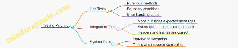
Integration Testing with Deterministic Inputs
Integration tests should avoid “wait and hope.” Use a test node that publishes known messages and a subscriber that captures outputs. Then assert on the captured messages.
A practical approach:
- Publish a sensor message with a fixed timestamp and frame.
- Spin the executor for a bounded time.
- Assert that exactly one output arrived and its header matches expectations.
Example: Integration Test Skeleton
// Pseudocode style for clarity.
// Arrange
auto input_pub = test_node->create_publisher<InMsg>("/in", qos);
std::optional<OutMsg> last;
auto sub = test_node->create_subscription<OutMsg>("/out", qos,
  [&](const OutMsg& msg){ last = msg; });

// Act
input_pub->publish(make_in_msg_fixed());
spin_some_until([&]{ return last.has_value(); }, 200ms);

// Assert
ASSERT_TRUE(last.has_value());
EXPECT_EQ(last->header.frame_id, "base_link");
EXPECT_NEAR(last->command_yaw, expected, 1e-6);
Advanced Details That Still Stay Simple
Parameters and Configuration
Treat parameters as inputs to core logic, not as hidden state. Load them once at startup, validate them, then pass validated values into the core component.
Time and Clocks
If your node uses time, inject a clock interface into core logic or pass timestamps explicitly. Tests become straightforward because you control time.
Error Reporting
Return structured status from core logic (for example, valid plus an error code). The node decides whether to publish a fallback command, publish nothing, or log a warning.
Mind Map: Error Handling Flow

Putting It Together
A clean, testable ROS 2 node looks like this: thin callbacks, explicit internal APIs, a message mapping layer, and a two-level test suite. When you follow that structure, debugging becomes less about guessing which callback did what, and more about checking a small set of deterministic transformations.
9.4 Add Parameters and Dynamic Reconfiguration for Field Tuning
Field tuning is the art of changing behavior without rebuilding the robot every time a cable is swapped, a camera is nudged, or a joint starts behaving slightly differently. In ROS 2, parameters give you a clean way to express “knobs,” and dynamic reconfiguration gives you a way to adjust those knobs while the system is running.
Foundational Parameter Design
Start by deciding which values are truly configurable. Good candidates are thresholds, gains, topic names, frame IDs, and model selection flags. Avoid putting high-frequency changing values into parameters; parameters are meant for configuration changes, not every control tick.
Use a consistent naming scheme so operators can find knobs quickly. A practical pattern is module.parameter_name, for example perception.confidence_threshold or control.kp. Keep units explicit in the parameter description, such as “meters” or “radians per second.”
Parameter Declaration and Validation
Declare parameters at node startup with defaults and descriptions. Then validate them before applying. Validation prevents the classic “it runs, but it’s wrong” situation.
A simple validation strategy:
- Range checks for numeric values (e.g.,
0.0 <= confidence_threshold <= 1.0). - Structural checks for strings (e.g., frame IDs must be non-empty).
- Cross-parameter checks (e.g.,
min_distance < max_distance).
Dynamic Reconfiguration Flow
Dynamic reconfiguration typically follows this sequence:
- Receive a parameter update request.
- Validate the new values.
- Apply changes to internal state.
- Confirm success or reject with a clear reason.
In ROS 2, you can implement this using parameter callbacks. The callback runs when parameters change, so keep it fast and deterministic. If applying changes requires expensive work (like reloading a model), consider splitting responsibilities: update a lightweight “desired config” parameter immediately, then trigger a separate action or service to perform heavy updates.
Mind Map: Parameter Strategy for Field Tuning
Example: Validated Parameter Callback in a Node
Below is a compact pattern for a node that tunes a perception threshold at runtime. The callback rejects invalid values and applies valid ones.
// Example: parameter callback with validation
class PerceptionTuner : public rclcpp::Node {
public:
  PerceptionTuner() : Node("perception_tuner") {
    this->declare_parameter<double>(
      "perception.confidence_threshold", 0.6,
      "Minimum confidence for detections in [0,1]");

    threshold_ = this->get_parameter("perception.confidence_threshold").as_double();

    cb_handle_ = this->add_on_set_parameters_callback(
      [this](const std::vector<rclcpp::Parameter> & params) {
        rcl_interfaces::msg::SetParametersResult res;
        res.successful = true;

        for (const auto & p : params) {
          if (p.get_name() == "perception.confidence_threshold") {
            double v = p.as_double();
            if (v < 0.0 || v > 1.0) {
              res.successful = false;
              res.reason = "confidence_threshold must be in [0,1]";
              return res;
            }
            threshold_ = v;
          }
        }
        return res;
      });
  }

private:
  double threshold_;
  OnSetParametersCallbackHandle::SharedPtr cb_handle_;
};
Example: Logging Applied Parameter Sets
When tuning in the field, you need an audit trail. Log the parameter values you actually applied, not just what you requested. A good practice is to log once per successful update, including the node name and the parameter key.
// Example: log after successful update
RCLCPP_INFO(this->get_logger(),
  "Applied perception.confidence_threshold=%.3f",
  threshold_);
Practical Tuning Workflow for Humanoid Robots
A systematic workflow keeps tuning from turning into guesswork:
- Start with safe defaults that avoid unstable behavior.
- Change one parameter at a time and observe the effect.
- Use consistent test conditions: same lighting, same distance, same stance.
- Record the parameter set that produced the best result.
For humanoids, tune control limits and safety-related parameters first, then perception thresholds, and finally any smoothing or filtering parameters. If you tune perception before safety limits, you may waste time chasing “bad detections” that are actually control saturation.
Mind Map: Common Parameter Categories for Humanoid Systems
Testing the Tuning Mechanism
Before trusting dynamic tuning, test the callback behavior:
- Unit test validation logic with boundary values.
- Integration test that a running node updates internal state correctly.
- Verify rejection paths return meaningful reasons.
This approach makes field tuning predictable: you can change parameters confidently, and when something goes wrong, the system tells you exactly why.
9.5 Write Unit And Integration Tests For Robot Software Components
Testing robot software is mostly about controlling uncertainty. Unit tests reduce uncertainty inside one package, while integration tests reduce uncertainty across packages, timing, and message contracts. For humanoid robots, the goal is simple: catch wrong assumptions early, before they become wrong motions.
Foundations: What to Test and Why
Start by classifying behavior into three buckets:
- Pure logic: math utilities, kinematics helpers, message formatting, parameter validation. These are ideal for fast unit tests.
- Stateful components: controllers, estimators, planners, safety monitors. These need unit tests that simulate inputs and verify outputs over time.
- System interactions: ROS 2 nodes, topics, services, actions, TF frames, and hardware interfaces. These are integration tests.
A practical rule: if you can run the test without ROS 2 middleware, it’s probably a unit test. If you need real message passing or TF, it’s probably an integration test.
Unit Testing Strategy for ROS 2 Packages
Unit tests should focus on contracts and invariants.
- Message contract invariants: verify fields, frame IDs, timestamps, and units. For example, if a function publishes a
geometry_msgs::msg::PoseStamped, test that it always setsheader.frame_idto the expected frame. - Deterministic math: test transforms, Jacobians, and constraint checks with fixed inputs.
- Boundary conditions: test saturation limits, NaN handling, and empty sensor data.
A simple example is testing a helper that converts a planned trajectory into controller commands.
#include <gtest/gtest.h>
#include "my_pkg/trajectory_to_commands.hpp"

TEST(TrajectoryToCommands, SetsUnitsAndSaturation) {
  auto cmd = my_pkg::trajectory_to_commands(
      /*time_s=*/1.0,
      /*pos_m=*/2.0,
      /*vel_m_s=*/100.0,
      /*max_vel_m_s=*/10.0);
  EXPECT_DOUBLE_EQ(cmd.velocity_m_s, 10.0);
  EXPECT_EQ(cmd.unit_tag, "m_s");
}
Integration Testing Strategy for ROS 2 Nodes
Integration tests verify that packages agree on how they talk.
Key targets for humanoid stacks:
- Topic wiring: publishers and subscribers match message types and QoS expectations.
- TF consistency: transforms exist, are connected, and use correct frame IDs.
- Timing behavior: callbacks handle message rates without dropping critical updates.
- Action and service semantics: goal acceptance, cancellation, and response fields.
Use a test node that plays the role of a sensor or planner. Feed known inputs, then assert outputs.
#include <gtest/gtest.h>
#include <rclcpp/rclcpp.hpp>
#include "std_msgs/msg/string.hpp"

TEST(Integration, TopicRoundTrip) {
  auto ctx = rclcpp::Context();
  rclcpp::init(0, nullptr, ctx);
  auto node = rclcpp::Node::make_shared("test_node");

  std::string received;
  auto sub = node->create_subscription<std_msgs::msg::String>(
    "in", 10,
    [&](const std_msgs::msg::String::SharedPtr msg){ received = msg->data; });

  auto pub = node->create_publisher<std_msgs::msg::String>("in", 10);
  rclcpp::executors::SingleThreadedExecutor exec;
  exec.add_node(node);

  std_msgs::msg::String m; m.data = "ok";
  pub->publish(m);
  exec.spin_some(std::chrono::milliseconds(50));

  EXPECT_EQ(received, "ok");
  rclcpp::shutdown(ctx);
}
Mind Map: Testing Layers and Responsibilities
Advanced Details Without the Usual Pain
- Use mocks for hardware: replace motor drivers with a fake that records commands and returns scripted joint states. Then unit-test safety logic by forcing encoder dropouts.
- Control time in tests: if a component uses
now(), inject a clock or wrap time access so tests can advance time deterministically. - Make failures actionable: when an assertion fails, include the expected frame ID, units, and the received values. A test that only says “mismatch” wastes time.
- Separate fast and slow suites: keep unit tests runnable in seconds, and integration tests runnable in minutes. That way developers actually run them.
A Cohesive Example Workflow
- Write unit tests for trajectory conversion and saturation.
- Write unit tests for controller update logic using synthetic joint states.
- Write an integration test that runs the controller node with a mock joint-state publisher.
- Add a TF-focused integration test that ensures the controller uses the correct base and end-effector frames.
This sequence catches mistakes early: wrong units in unit tests, wrong control behavior in stateful unit tests, and wrong wiring or frame usage in integration tests. The robot stays boring, which is the best kind of robot behavior.
10. Simulation to Hardware Transfer with Gazebo and System Testing
10.1 Build URDF and Validate Kinematics and Visuals in Simulation
A URDF is the contract between your robot’s geometry, its joints, and the transforms your software will trust. In simulation, wrong frames or mismatched visuals don’t just look odd; they break control, localization, and collision behavior. The goal of this section is to make the URDF internally consistent so that kinematics and visuals agree with each other and with ROS 2 expectations.
Start with a Clean Frame Strategy
Before writing links and joints, decide how you will name and orient frames. A practical rule is to keep one “world-like” frame (often base_link as the root) and ensure every joint defines a transform that maps parent link coordinates into child link coordinates.
Use these checks as you build:
- Every joint has an
originwith a clear meaning: position and orientation of the child frame relative to the parent frame. - Every link has at least one visual and collision element, even if collision is simplified.
- The root link is consistent with how you will publish TF later.
Define Links with Geometry That Serves Two Purposes
URDF links typically contain:
- Visual: what you see in simulation.
- Collision: what physics uses.
For humanoids, visuals can be detailed, but collision should be conservative and stable. A common approach is to use primitive shapes (boxes, cylinders, spheres) for collision and keep meshes for visuals.
A good sanity test: if you can’t explain why a collision shape is placed where it is, it will eventually cause “mysterious” contacts.
Specify Joints with Correct Axes and Limits
Joints define kinematics. For each joint:
- Choose the joint type (
revolute,continuous,prismatic,fixed). - Set
axisin the joint frame, not in some global frame. - Provide
limitfor revolute joints so simulation and controllers have meaningful bounds.
A frequent humanoid mistake is defining an axis that looks right in a CAD model but is wrong once you account for the URDF joint frame orientation.
Validate Kinematics Before You Care About Looks
Visual correctness is useful, but kinematic correctness is mandatory. Validate in this order:
- TF tree structure: the parent-child relationships match your intended kinematic chain.
- Joint axes: when you command a joint, the motion direction matches expectations.
- Transform magnitudes: link lengths and offsets match the robot’s physical proportions.
- Inertia sanity: mass and inertia values are positive and roughly consistent with geometry scale.
Validate Visuals Without Breaking Physics
Once kinematics are correct, align visuals:
- Ensure mesh scale matches your URDF units.
- Confirm that the mesh origin aligns with the link frame.
- Keep visual orientation consistent with collision orientation so that debugging is less confusing.
If visuals appear rotated relative to collision, it usually means the mesh is authored in a different coordinate system than the link frame.
Mind Map: URDF for Humanoid Kinematics and Visuals
Example: Minimal Joint with Visual and Collision
<link name="upper_arm_link">
  <visual>
    <origin xyz="0 0 0" rpy="0 0 0"/>
    <geometry><cylinder radius="0.04" length="0.25"/></geometry>
  </visual>
  <collision>
    <origin xyz="0 0 0" rpy="0 0 0"/>
    <geometry><cylinder radius="0.04" length="0.25"/></geometry>
  </collision>
</link>

<joint name="shoulder_pitch" type="revolute">
  <parent link="torso_link"/>
  <child link="upper_arm_link"/>
  <origin xyz="0.12 0.0 0.35" rpy="0 0 0"/>
  <axis xyz="0 1 0"/>
  <limit lower="-1.57" upper="1.57" effort="30" velocity="2"/>
</joint>
This example keeps visuals and collision aligned by using the same primitive geometry and origin. For a humanoid, that reduces debugging time when you first verify motion direction.
Example: A Systematic Validation Checklist
Validation Checklist
- Load URDF in the simulator
- Inspect TF tree for expected parent-child links
- Rotate one joint at a time
- Confirm motion direction matches joint axis
- Confirm rotation center matches joint origin
- Compare visual and collision alignment
- If they differ, fix mesh origin or scale
- Check inertia values
- No negative or zero mass
- Inertia magnitudes roughly match link size
- Confirm limits prevent impossible poses
Practical Tips for Humanoid Chains
Humanoids have many joints, so consistency matters more than cleverness. Keep joint naming aligned with your controller interfaces, and ensure each joint’s axis is defined once and reused conceptually across the model. When you validate, do it in small segments: torso to hip, hip to knee, knee to ankle, then repeat for the other leg and the arms.
By the end of this step, your simulation should show a robot that moves in the right directions, rotates around the right centers, and looks like the same robot your controllers assume. That’s the foundation you need before you start tuning behavior in later sections.
10.2 Configure Sensors in Simulation to Match Real Hardware Outputs
A simulation that “looks right” but measures differently will quietly ruin your whole pipeline. The goal here is not perfect physics; it’s consistent sensor behavior so your perception, estimation, and control code sees the same kinds of inputs it will see on the robot. The workflow below moves from foundational alignment to advanced calibration details, with concrete checks at each step.
Start with Sensor Contracts and Coordinate Frames
Before touching parameters, define what each sensor publishes and what frame it claims. In ROS 2, that means message fields plus TF frames. For example, a camera image topic should specify its optical frame, and an IMU message should state its orientation frame and angular velocity axes.
A practical rule: every sensor gets a “contract” document with three items: (1) frame IDs, (2) units and axis conventions, and (3) timing behavior. If your IMU in simulation publishes in sensor_msgs/Imu with angular_velocity in rad/s and linear_acceleration in m/s², your real IMU must match those units and axes after any driver conversions.
Match Geometry and Mounting with URDF and TF
Sensor mismatch often comes from mounting transforms, not from the sensor model itself. Ensure the URDF links for the sensor are correct and that the TF tree in simulation matches the real robot’s TF tree.
Concrete example: if your camera is rotated 90° around its optical axis in the real mount, but the URDF uses a different rotation, your detections will appear shifted even if the image pixels are perfect. Fixing this is usually faster than compensating later in perception.
Calibrate Intrinsics and Distortion for Cameras
Simulation cameras should reproduce the same projection model used by your real camera pipeline. If your real camera uses a pinhole model with radial-tangential distortion, configure the same intrinsics (fx, fy, cx, cy) and distortion coefficients.
Concrete example: if your real pipeline undistorts images before publishing, then your simulation should publish either (a) raw distorted images plus the same undistortion node, or (b) already-undistorted images with matching intrinsics for downstream nodes. Mixing these choices causes subtle scale and edge errors.
Reproduce Noise, Bias, and Quantization
Real sensors are not just “truth plus Gaussian noise.” IMUs have bias drift and axis-dependent noise; depth sensors have structured error; encoders have quantization.
For IMUs, configure:
- Constant bias per axis (initial offset)
- Noise density (random walk behavior)
- Update rate and timestamp jitter
For depth or stereo, configure:
- Depth noise as a function of range
- Missing data rate and invalid pixel patterns
Concrete example: if your estimator expects occasional IMU spikes and you simulate perfectly smooth IMU data, your filter may become overconfident and reject real-world corrections.
Match Timing and Synchronization Behavior
Timing mismatches are a top cause of “it works in sim” failures. Ensure:
- Sensor publish rates match the real device
- Timestamps reflect the same reference (sensor time vs system time)
- Latency between sensor measurement and message publication is modeled consistently
Concrete example: if your real camera driver buffers frames and publishes with ~30 ms delay, but simulation publishes immediately, your time alignment with TF and other sensors will be off. Your fusion node may still run, but it will fuse the wrong pose with the wrong image.
Validate with Targeted Experiments
Use small, repeatable tests that isolate each sensor.
- Camera test: publish a static calibration target and verify pixel reprojection error after your full image pipeline.
- IMU test: place the robot in known orientations and compare gravity vector magnitude and axis signs.
- Odometry test: run a short motion and compare wheel/leg encoder-derived velocities and integrated displacement.
If you can’t explain a mismatch with a single parameter category (frames, units, intrinsics, noise, or timing), you haven’t isolated enough yet.
Mind Map of Sensor Matching Steps
Mind Map: Configure Sensors in Simulation to Match Real Hardware Outputs
Example Configuration Checklist for a Camera and IMU
Use this checklist when you configure simulation sensor plugins and ROS 2 nodes.
- Camera
- Frame ID matches URDF optical frame
- Intrinsics match real calibration
- Distortion model matches real pipeline
- Publish rate matches driver
- Timestamp delay matches driver behavior
- IMU
- Frame ID matches IMU mounting frame
- Axes match driver output conventions
- Bias and noise match measured statistics
- Timestamping matches driver behavior
- Gravity magnitude matches expected units
When these items are aligned, your perception and estimation modules stop compensating for sensor lies, and your robot behavior becomes easier to debug because the inputs are finally honest.
10.3 Run End to End Scenarios for Perception Estimation and Control
End-to-end scenarios connect three things that often get tested separately: what the robot sees, what it believes about its state, and what it does next. The goal is not to prove perfection; it’s to verify that the interfaces between modules behave correctly under realistic timing, noise, and message flow.
Scenario Foundations
Start by defining a single, repeatable scenario with measurable acceptance criteria. For a humanoid, a practical example is “approach a target, estimate pose, then execute a safe reach.” Break the scenario into phases so you can pinpoint failures:
- Perception phase: camera frames produce target detections with timestamps.
- Estimation phase: detections plus IMU and joint states produce a consistent robot and target pose.
- Control phase: the controller converts pose into joint commands while respecting limits.
A good scenario includes constraints that force integration issues to show up. For example, require the robot to keep balance while the target moves slightly, and ensure the perception pipeline runs at a different rate than the control loop.
Mind Map: End to End Scenario Flow
Integrated Example: Approach and Reach
Use a concrete message contract so each module knows what it’s responsible for. For instance, perception publishes a detection message containing:
target_posein the camera frame (or a known intermediate frame)timestampfrom the image acquisition timeconfidenceand astatusfield (valid, occluded, lost)
Estimation subscribes to that message and performs two checks before fusing:
- Transform availability: the required TF transforms exist for the detection timestamp.
- Data consistency: joint states and IMU are recent enough to avoid mixing old state with new perception.
If either check fails, estimation publishes a “no update” or “stale” status rather than silently producing a pose. That one decision prevents control from chasing ghosts.
Control then consumes the estimated target pose and computes a task-space goal. For whole-body control, the controller should also verify feasibility:
- The goal is within reach given current joint limits.
- The planned motion respects balance constraints.
- The command rate and magnitude stay within safe bounds.
A simple acceptance criterion for the example scenario:
- The target pose estimate becomes stable within a tolerance after a short settling period.
- The controller reaches the reach posture without violating joint limits.
- During occlusion, the controller either holds position or transitions to a safe behavior based on the estimation status.
Systematic Test Steps
- Dry run with recorded inputs: record camera, IMU, and joint states while running a short session. Replay it to ensure deterministic behavior in the software stack.
- Perception-only verification: confirm detection timestamps align with the image stream and that the detection message contract is consistent across frames.
- Estimation-only verification: validate TF usage by checking that the target pose in the world frame changes smoothly when the target moves.
- Control integration: run the full loop and verify that control never consumes an invalid estimation status.
- Fault injection: simulate one failure at a time, such as dropping detection messages for a brief interval or forcing a TF lookup to fail, and confirm the system degrades gracefully.
Timing and Interface Checks
Integration failures often come from time. Add explicit checks in your scenario harness:
- Timestamp freshness: reject perception updates older than a threshold relative to the current state.
- Transform timestamp alignment: ensure TF lookups use the detection timestamp, not “now,” unless you intentionally model latency.
- Rate mismatch handling: if perception runs slower than control, hold the last valid estimate and mark its age in diagnostics.
Minimal Scenario Harness Example
The following pseudocode shows the core logic for gating control on estimation validity.
loop at control_rate:
  est = get_latest_estimation()
  if est.status != VALID:
    send_hold_or_safe_command()
    log("estimation invalid", est.status, est.age_ms)
    continue

  if est.age_ms > MAX_AGE_MS:
    send_hold_or_safe_command()
    log("estimation stale", est.age_ms)
    continue

  goal = compute_task_goal(est.target_pose)
  cmd = whole_body_controller(goal, current_state)
  cmd = apply_safety_limits(cmd)
  publish_joint_commands(cmd)
What “Done” Looks Like
A scenario run is successful when logs show a coherent chain: detections are produced with correct timestamps, estimation publishes consistent poses with clear validity status, and control issues feasible commands that match the scenario intent. When something goes wrong, the failure should be attributable to a specific phase rather than a vague “it didn’t work” outcome.
10.4 Calibrate Simulation Parameters to Reduce Reality Gaps
Reality gaps happen because simulation is a polite liar: it assumes perfect timing, ideal sensors, and clean physics. Calibration makes the simulation stop lying in the specific ways that matter for your humanoid pipeline—perception, state estimation, and control.
Start with a Gap Inventory
Before changing numbers, list the mismatches you can observe. Use a simple table to connect symptoms to likely causes.
| Symptom in Hardware | What It Usually Means | First Parameter To Check |
|---|---|---|
| Pose drifts faster than expected | IMU bias or noise model mismatch | IMU noise, bias random walk |
| Foot contact timing is off | Contact friction or contact thresholds | friction, restitution, contact solver |
| Joint tracking overshoots | Motor dynamics or controller gains mismatch | actuator limits, damping, PID gains |
| Vision detections “jump” | Image noise, exposure, motion blur mismatch | camera noise, rolling shutter |
A good practice is to record one short run in simulation and one on hardware with the same motion script, then compare time-aligned logs.
Calibrate Kinematics and Frames First
If frames are wrong, everything downstream becomes “calibration” that never converges.
- Verify URDF link lengths and joint axes by checking static transforms in TF.
- Confirm the origin of each sensor frame relative to the robot base.
- Validate joint limits and default poses by commanding a known configuration and comparing measured joint angles.
A quick sanity check: publish a static transform chain and ensure the end-effector pose matches the expected geometry within a small tolerance.
Calibrate Sensor Models with Measured Statistics
Sensors rarely fail because their mean is wrong; they fail because their noise and timing are wrong.
IMU calibration
- Estimate bias by holding the robot still for a few seconds and averaging readings.
- Estimate noise by computing variance after removing the mean.
- In simulation, set the IMU bias and noise parameters to match those statistics.
Camera calibration
- Match intrinsics and distortion to your real camera.
- Add realistic image noise and exposure effects so detection confidence behaves similarly.
- If your camera uses rolling shutter, model the readout delay so fast head or arm motions don’t create systematic skew.
Encoders and joint states
- Set encoder quantization and update rate to match hardware.
- Add small latency if your hardware pipeline buffers messages.
Calibrate Physics for Contact and Actuation
Humanoid behavior is dominated by contact. If contact is off, the rest is just paperwork.
Friction and restitution
- Start with a single surface material and tune friction so the slip behavior matches.
- Tune restitution only if you see bounce-like behavior; many humanoids should look “sticky,” not springy.
Contact solver settings
- Adjust contact stiffness and damping to match penetration depth and settling time.
- Ensure the simulation timestep is small enough that contact events are resolved consistently.
Actuator dynamics
- Model motor limits, gearbox friction, and joint damping.
- If your controller saturates in hardware, it should saturate in simulation too, or your tuning will lie.
Use a Two-Stage Calibration Loop
Calibrate in layers so you don’t chase moving targets.
- Open-loop matching: drive joints with recorded commands and tune sensor and actuator models until joint trajectories match.
- Closed-loop matching: enable full estimation and control, then tune contact and noise parameters until the system stays stable.
Keep the loop measurable: define acceptance thresholds such as “foot contact occurs within ±20 ms” or “base pitch error stays under 2 degrees for 10 seconds.”
Mind Map: Calibration Workflow
Example: Calibrating Foot Contact Timing
Suppose your humanoid’s foot lands late in simulation.
- Compare contact event timestamps: detect contact in both logs using force/torque thresholds.
- If simulation contacts earlier, reduce effective friction or increase contact damping so the foot “sticks” less aggressively.
- If simulation contacts later, check contact thresholds and solver stiffness; a too-soft contact model can delay force buildup.
- Re-run with the same timestep and controller gains to isolate the effect.
After each change, verify that the base pose and joint tracking remain within tolerance; contact tuning can accidentally mask actuator issues.
Example: Calibrating IMU Bias for State Estimation
If your estimated roll angle drifts during a stationary hold:
- Measure average IMU bias on hardware.
- Set the same bias in simulation.
- Match noise variance so the filter’s confidence behaves similarly.
- Re-run the stationary test and confirm drift rate drops to the expected level.
Once the stationary case matches, move to slow motion where bias and noise both matter, then proceed to faster motions.
Practical Guardrails
- Change one parameter group at a time and keep a record of the exact values.
- Use consistent random seeds for noise so differences are attributable.
- Keep simulation timestep fixed during a calibration run; changing it midstream makes comparisons meaningless.
Calibration is not a one-time chore. It’s a disciplined loop that turns “simulation seems close” into “simulation behaves like the robot we actually built.”
10.5 Perform System Level Tests with Repeatable Test Scripts
System-level tests answer a simple question: when the whole humanoid stack runs together—sensors, transforms, perception, estimation, planning, control, and actuation—does it behave the way the robot’s safety and performance requirements demand? Repeatable test scripts make this question answerable on every build, not just on the day everything works.
Foundational Test Principles
Start by defining what “system-level” means for your robot. For a humanoid, it usually includes at least one full loop from sensor input to actuator output, plus the timing and frame consistency that glue the loop together.
A repeatable test script should:
- Produce the same inputs each run, either by replaying recorded sensor data or by using deterministic test fixtures.
- Check outcomes with explicit pass/fail criteria, not by eyeballing plots.
- Capture evidence automatically: logs, key metrics, and artifacts like bag files or screenshots.
- Fail fast with actionable messages, so a broken transform or a controller saturation shows up immediately.
Test Scope and Success Criteria
Pick a small set of scenarios that cover the failure modes you can’t afford to miss. For example:
- Standing stability: the robot maintains balance while receiving nominal sensor streams.
- Reach and touch: the end-effector reaches a target and the contact event occurs within a tolerance.
- Recovery behavior: when a sensor stream drops or a controller limit is hit, the system transitions to a safe state.
For each scenario, define measurable criteria. Examples:
- Pose error: end-effector position error under a threshold for a time window.
- Timing: perception-to-control latency under a maximum, measured from message timestamps.
- Frame validity: TF lookups succeed for required frames at a minimum rate.
- Actuation sanity: commanded joint velocities remain within configured bounds.
Mind Map: System Test Script Design
Building the Script: A Practical Workflow
- Create a scenario manifest: list required nodes, topics, frames, and the expected outputs. This prevents “it worked on my machine” drift.
- Use a deterministic input source: prefer recorded bags for perception and estimation tests. For control-only checks, use scripted joint state publishers.
- Gate on readiness: the script should wait until TF is publishing, required topics are active, and controllers report they are in the correct state.
- Run the scenario with a fixed time window: for example, 30 seconds of standing, then 10 seconds of reach.
- Collect metrics continuously: sample at a consistent rate and store results even if the test fails.
- Assert at the right granularity: check frame availability continuously, but check end-effector error over a stable interval to avoid transient noise.
Example: Repeatable Standing Stability Test
Assume you have recorded a bag named stand_nominal_2026-02-15.bag and your system publishes:
/tffor frame transforms/joint_states/cmd_joint_positions/end_effector_pose(or an equivalent pose topic)
Your script should:
- Verify TF lookups for
base_linktoworldandend_effectortobase_linkat least 95% of the time during the window. - Verify commanded joint positions do not exceed configured limits.
- Verify end-effector pose remains within a small drift envelope during standing.
Example: Recovery Test for Sensor Drop
For a recovery scenario, you want to test behavior when inputs degrade. A repeatable approach is to replay a bag but pause one sensor topic for a controlled duration.
Pass criteria might include:
- The system transitions to a safe controller mode within a maximum time.
- Actuation commands stop changing rapidly, or switch to a hold strategy.
- Logs include a specific error signature that your runbook can interpret.
Mind Map: Assertions and Evidence
Advanced Details That Prevent “False Passes”
- Use time-windowed assertions: a single good sample doesn’t mean the system is stable.
- Check timestamp consistency: if sensor timestamps and system clock drift, your latency metrics and fusion results can look fine while the robot is actually acting on stale data.
- Validate message contracts: confirm required fields are present and units are consistent, especially for pose and contact signals.
- Record configuration hashes: include controller parameters and model files so a passing run can be reproduced exactly.
Minimal Script Output Checklist
Every run should produce:
- A single-line summary with scenario name and pass/fail.
- A metrics file with the key thresholds and measured values.
- A log bundle containing TF warnings, controller state transitions, and any safety triggers.
Repeatable system tests turn integration from a guessing game into a measurable process. When something breaks, you should know whether it’s a transform issue, a timing issue, a controller limit issue, or a perception-to-estimation mismatch—usually within the first few minutes of reading the artifacts.
11. Deployment on Jetson with Containers and Performance Profiling
11.1 Package Applications for Deployment with Containers
Containers help you ship a robot software stack with fewer “works on my machine” surprises. For Jetson-based humanoid systems, the goal is simple: keep the runtime environment consistent, keep hardware access explicit, and keep startup behavior predictable.
Container Foundations for Robot Deployment
A container image is an immutable filesystem plus a startup command. At runtime, you attach it to the robot’s devices (camera, IMU, serial buses), networks, and sometimes GPU acceleration. The practical best practice is to treat the container as the unit of deployment, while keeping configuration outside the image.
Start by separating three concerns:
- Build-time dependencies: compilers, ROS 2 build tools, Python packages used only during build.
- Runtime dependencies: ROS 2 runtime, your nodes, shared libraries, and any model files you truly need at startup.
- Runtime configuration: parameters, launch choices, network settings, and device mappings.
A clean separation reduces rebuild time and makes it easier to reproduce a known-good image.
Image Design That Stays Maintainable
Use a multi-stage build so the final image contains only what runs. In practice, you build your workspace in one stage, then copy the install artifacts into a smaller runtime stage.
Also decide what should be inside the image:
- Put compiled ROS 2 packages in the image.
- Put static assets (URDFs, calibration files that rarely change) in the image.
- Put tunable parameters and robot-specific calibration outside the image, mounted at runtime.
For humanoids, this matters because calibration and tuning often change between robots and even between test sessions.
Mind Map: Container Packaging Decisions
Example: Minimal Container Layout for ROS 2
A practical layout keeps the container entrypoint simple: source the ROS environment, then run a launch file. Your launch file should reference parameters from mounted paths.
# Stage 1: build
FROM ros:humble AS builder
WORKDIR /ws
COPY src ./src
RUN apt-get update && apt-get install -y python3-colcon-common-extensions
RUN . /opt/ros/humble/setup.sh && colcon build --merge-install

# Stage 2: runtime
FROM ros:humble
WORKDIR /ws
COPY --from=builder /ws/install /ws/install
ENV ROS_DISTRO=humble
ENV PATH=/ws/install/bin:$PATH
ENTRYPOINT ["bash", "-lc", "source /opt/ros/$ROS_DISTRO/setup.bash && source /ws/install/setup.bash && ros2 launch my_pkg robot.launch.py"]
This example assumes your launch file is stable and your parameters are mounted at runtime. If you need different launch variants, prefer passing arguments to the entrypoint rather than rebuilding images.
Example: Runtime Configuration via Mounts
Mount a configuration directory so you can swap parameters without rebuilding. A typical pattern is:
/configmounted from the host- launch file reads
*.yamlfrom/config
docker run --rm -it \
  --network host \
  -v /path/to/robot_config:/config:ro \
  --device=/dev/video0 \
  --device=/dev/ttyUSB0 \
  my-robot-image:1.0
Using --network host is often the least surprising choice for ROS 2 discovery on a single robot network. If you later need stricter networking, you can adjust, but start with predictable behavior.
GPU Access and Deterministic Performance
Jetson acceleration typically requires exposing GPU-related runtime hooks. The key packaging rule is to keep the runtime stage aligned with the Jetson software stack so CUDA libraries match what the host provides.
In practice, you validate GPU usage by running a small perception node inside the container and checking that it can load the expected acceleration libraries. If it falls back to CPU, you want to know immediately rather than after a long integration run.
Startup Reliability and Observability
Containers should log to stdout/stderr so you can inspect behavior with standard tooling. Add a simple health check strategy in your launch flow: confirm that critical topics are publishing (for example, /joint_states and the primary perception output) and that transforms are available.
A good rule is: if the container starts but the robot cannot move or perceive, the logs should clearly say why. That means your nodes should fail loudly on missing configuration files, missing model assets, or unavailable devices.
Mind Map: Deployment Checklist
Practical Packaging Outcome
When you package this way, you get three concrete benefits: you can reproduce the same software environment across test benches, you can update parameters without rebuilding, and you can debug startup issues using consistent logs. That’s the foundation you need before you start tuning control loops and perception pipelines for a humanoid robot.
11.2 Configure GPU and Device Access for Jetson Runtime Environments
Jetson runtime environments usually fail in predictable ways: the container starts, but the GPU is invisible; the camera device exists, but permissions block access; or the process runs with the wrong libraries and silently falls back to CPU. This section focuses on making those failure modes impossible by construction.
Foundations: What Must Be True at Runtime
A working robot runtime needs three categories of access:
- GPU access so CUDA and related libraries can be used by perception and inference nodes.
- Device access for cameras, IMUs, serial buses, and any GPIO or actuator controllers.
- Library compatibility so the runtime uses the same ABI expectations as the host drivers.
A practical rule: treat the host as the source of truth for drivers, and treat the container as the source of truth for application code.
GPU Access with Container Runtimes
On Jetson, GPU support depends on the host driver stack. In practice, you configure the container runtime to pass through the GPU devices and required libraries.
Checklist for GPU visibility
- Confirm the host can see the GPU.
- Confirm the container can see the GPU.
- Confirm your inference stack is actually using the GPU (not just importing CUDA libraries).
Example: verify GPU visibility inside the container
# Run Inside the Container Shell
nvidia-smi || true
# Jetson May Not Provide Nvidia-Smi; Use CUDA Tooling Instead
python3 - <<'PY'
import torch
print('torch', torch.__version__)
print('cuda available', torch.cuda.is_available())
if torch.cuda.is_available():
    print('device', torch.cuda.get_device_name(0))
PY
If cuda available is false, the container is missing GPU device access or the CUDA libraries don’t match the host.
Device Access for Cameras and Sensors
Device access is mostly about two things: mapping the correct device nodes and granting permissions that match the process user.
Common device categories
- Video devices:
/dev/video*for cameras. - USB serial:
/dev/ttyUSB*or/dev/ttyACM*for sensors. - I2C and SPI:
/dev/i2c-*and/dev/spidev*for low-level peripherals.
Example: map devices and run as a user that can read them
# Illustrative Run Command
docker run --rm -it \
  --network host \
  --runtime nvidia \
  --gpus all \
  -v /dev:/dev \
  -e NVIDIA_VISIBLE_DEVICES=all \
  -e NVIDIA_DRIVER_CAPABILITIES=all \
  your_ros2_image:tag \
  bash
Mapping all of /dev is convenient for early bring-up, but for production you should map only the needed device nodes to reduce accidental access.
Permissions and User Identity
A container process often runs as root by default, which “works” but hides permission problems that will later bite you when you switch to a non-root user.
Best practice
- Create a non-root user in the container.
- Ensure that user can access the mapped device nodes.
- Keep group IDs aligned with the host where possible.
Example: check device permissions
ls -l /dev/video* 2>/dev/null || true
ls -l /dev/ttyUSB* /dev/ttyACM* 2>/dev/null || true
id
If the device files are owned by a group your container user does not belong to, ROS 2 camera nodes will fail to open the stream.
Library Compatibility and Environment Variables
GPU libraries must match the host driver expectations. The safest approach is to avoid bundling driver components inside the container and instead rely on the runtime to provide them.
Practical checks
- Confirm that the container sees the expected CUDA version.
- Confirm that your inference runtime loads the correct backend.
- Ensure that environment variables used by your inference stack are set consistently across dev and deployment.
Mind Map: Runtime Access Checklist
Integrated Validation Flow
Run a short, ordered validation before you start the full humanoid stack:
- GPU smoke test: run a tiny script that checks CUDA availability.
- Camera smoke test: start the camera node and confirm frames arrive.
- Sensor smoke test: open the serial device and confirm messages parse.
- ROS 2 integration check: verify that the nodes publish and subscribe on the expected topics.
This sequence prevents chasing ghosts like “the perception model is slow” when the real issue is that the container is silently running on CPU.
Example: Minimal Runtime Configuration Strategy
Keep the runtime configuration minimal and explicit: pass through GPU support, map only the required device nodes, run as a non-root user, and validate with small tests before launching the full system. That approach makes failures immediate and understandable, which is exactly what you want when you’re debugging a humanoid robot that has places to be.
11.3 Set Up Logging Monitoring and Health Checks on the Robot
A good robot log is boring in the best way: it tells you what happened, when it happened, and what component decided it. On Jetson, the goal is to keep logs structured enough to search, lightweight enough to run continuously, and consistent enough that you can correlate events across ROS 2 nodes.
Foundations for Useful Robot Logs
Start with three decisions that prevent chaos later.
- Define log levels by intent:
DEBUGfor developer detail,INFOfor state changes,WARNfor recoverable problems,ERRORfor failed operations, andFATALfor conditions that should stop the system. - Use consistent fields: include
node,component,event, and a stable identifier likerobot_idorsession_id. When you later grep, you’ll thank yourself. - Pick a timestamp source: prefer ROS 2 time when you need correlation with sensor data, otherwise use system time for operational events. Mixing them without a label makes timelines lie.
Logging Architecture in ROS 2 and Jetson
In ROS 2, each node can emit logs, and you can also capture system-level signals from the OS. A practical setup uses both:
- ROS 2 logs for message flow, controller decisions, and perception outcomes.
- System logs for CPU pressure, memory exhaustion, device errors, and network issues.
A simple rule: if the event affects robot behavior, it belongs in ROS 2 logs; if it affects resource availability, it belongs in system logs.
Mind Map: Logging and Health Checks
Health Checks That Catch Real Failures
Health checks should answer three questions: Is the node alive? Is the data usable? Is the control loop healthy?
Heartbeat and Liveness
Implement a lightweight heartbeat topic or service response. The monitoring process expects a message every N seconds. If it stops, you treat it as a failure even if the node process still exists.
Data Usability Checks
For perception and state estimation, “alive” isn’t enough. Add checks like:
- Sensor stream rate above a minimum.
- TF tree available for required frames.
- Pose covariance within expected bounds.
These checks prevent silent degradation where everything runs but the robot becomes confused.
Control Loop Health Checks
For control, check:
- Loop frequency near target.
- Command age not exceeding a maximum.
- Actuator feedback arriving within a timeout.
If commands are being generated but feedback is missing, you want to stop rather than keep guessing.
Example: Minimal ROS 2 Health Publisher
This example publishes a heartbeat with structured fields. Keep it small so it doesn’t become the bottleneck.
import rclpy
from rclpy.node import Node
from std_msgs.msg import String
import time

class HealthNode(Node):
    def __init__(self):
        super().__init__('health_node')
        self.pub = self.create_publisher(String, '/robot/health', 10)
        self.robot_id = 'humanoid-01'
        self.session_id = '2026-02-15'
        self.timer = self.create_timer(1.0, self.tick)

    def tick(self):
        msg = {
            'robot_id': self.robot_id,
            'session_id': self.session_id,
            'node': 'health_node',
            'event': 'heartbeat',
            't_system': time.time()
        }
        self.pub.publish(String(data=str(msg)))

rclpy.init()
node = HealthNode()
rclpy.spin(node)
A monitoring component can parse the message and alert when heartbeats stop for more than, say, 3 seconds.
Example: Health Monitoring with Clear Actions
Use a single policy table: condition → action. For example:
- Missing heartbeat → restart node → if repeated, enter safe mode.
- Sensor rate below threshold → reduce processing rate → warn operator.
- Control loop frequency low → stop motion and hold position.
Here’s a compact policy sketch.
POLICY = [
  ('heartbeat_missing', 3.0, 'restart_node'),
  ('sensor_rate_low',  0.5, 'throttle_and_warn'),
  ('control_loop_late', 0.2, 'stop_motion_hold'),
]

def decide(action_inputs):
    # Action_inputs Contains Computed Health States
    # return one action string
    return 'stop_motion_hold'
Operational Practices That Make Monitoring Work
- Log rotation and retention: keep a rolling window so storage doesn’t silently fill.
- Separate debug from runtime: don’t run
DEBUGpermanently; it creates noise and hides the important lines. - Correlate with identifiers: include
session_idin every critical log so you can filter a single run. - Treat WARN as data: count WARN occurrences per node; a rising trend often precedes a failure.
When logging, monitoring, and health checks are aligned, you get a system that explains itself. It won’t prevent every fault, but it will help you respond quickly and correctly—without guessing which component is lying.
11.4 Profile CPU GPU and Memory Usage for Bottleneck Identification
Profiling on Jetson is mostly about asking three questions in the right order: what is consuming time, what is consuming memory, and what is causing the two to misbehave together. If you start with memory first, you often end up chasing symptoms; if you start with CPU time first, you can usually narrow the search to a few hot paths quickly.
Foundations for Bottleneck Thinking
Begin by defining the measurement window and the workload. For a humanoid demo, pick one representative run: a short perception-to-motion cycle (for example, “detect person, estimate pose, plan reach, execute 1–2 seconds”). Keep the robot in the same posture and use the same camera exposure settings so the workload stays comparable.
Next, separate “where time goes” from “where bytes go.” CPU time typically maps to callback execution, preprocessing, message serialization, and scheduling overhead. GPU time maps to inference kernels, image transforms, and any CUDA-accelerated preprocessing. Memory usage maps to buffers, message queues, tensor allocations, and fragmentation from repeated allocations.
Finally, decide what “bottleneck” means for your system. If control commands arrive late, CPU scheduling or synchronization is likely. If perception drops frames, GPU saturation or memory pressure is likely. If the system slows down over time, memory growth or allocator churn is likely.
Mind Map: Profiling Workflow
CPU Profiling: Find the Hot Paths
Start with CPU usage at the process level, then move to threads, then to functions. Look for one of three patterns: a single thread pegged near 100%, many threads with moderate usage but long callback durations, or frequent context switching.
In ROS 2, long callback durations are often caused by doing heavy work inside subscription callbacks. A practical rule: keep callbacks short and push heavy computation to a dedicated worker thread or a separate node. For example, instead of running image preprocessing and inference inside the camera subscription callback, publish the raw image (or a lightweight preprocessed representation) and let an inference node handle the expensive steps.
Also check serialization overhead. If you publish large images at high rate, serialization and copying can dominate CPU time. A common mitigation is to reduce message size by using compressed transport or by publishing only the fields needed for downstream steps.
GPU Profiling: Separate Compute from Transfers
GPU bottlenecks usually show up as either high kernel time or high data transfer time. If kernel time is high, you are compute-bound; if transfer time is high, you are moving too much data or moving it too often.
A concrete example: if you convert images between formats on the CPU and then upload to the GPU, you may pay both CPU conversion cost and GPU transfer cost. Prefer a single conversion path that matches the inference input format, and keep preprocessing on the GPU when it reduces total copies.
Watch for GPU idle gaps. If the GPU is frequently idle while CPU is busy, the CPU may be starving the GPU by preparing inputs too slowly. If CPU is idle while GPU is busy, you are likely compute-bound and should focus on kernel efficiency and batch sizing.
Memory Profiling: Peak, Growth, and Queue Pressure
Memory issues come in three flavors: high peak usage, steady growth, and sudden spikes. High peak usage can cause swapping or allocator pressure. Steady growth often indicates buffers that are not released or queues that retain old messages. Sudden spikes often correlate with bursts in message rates or temporary allocations during preprocessing.
In ROS 2, queue depth matters. If a perception node publishes faster than the consumer can process, messages accumulate in queues, increasing memory usage and adding latency. Use QoS settings intentionally: for sensor streams, a “keep last” policy with a small depth often prevents unbounded backlog. Then verify with profiling that the consumer’s callback duration fits within the expected cycle time.
Preallocation helps. If your pipeline repeatedly allocates tensors or intermediate buffers per frame, allocator churn can inflate CPU time and memory fragmentation. Reuse buffers where possible and keep tensor shapes stable for the duration of a run.
Example: Correlate Symptoms to Causes
Suppose you observe: CPU usage is moderate, GPU utilization is high, and memory peaks near a limit during inference. The likely cause is that each frame triggers large temporary allocations on the GPU or frequent CPU-to-GPU transfers. The fix path is systematic: reduce intermediate tensor sizes, ensure preprocessing produces the exact inference input format, and reuse buffers so peak memory drops and allocator churn decreases.
Suppose instead you observe: CPU usage spikes, GPU utilization drops, and memory grows slowly. That pattern often indicates the CPU is spending time handling backlog or serialization while the GPU waits for inputs. The fix is to reduce message size, shorten callbacks, and tune QoS queue sizes so the pipeline stays real-time.
Practical Checklist for Bottleneck Identification
- Run one representative demo cycle and record CPU, GPU, and memory metrics for the same time window.
- Identify the top CPU threads and the longest callback durations.
- Determine whether GPU time is dominated by kernels or transfers.
- Check whether memory is peaking once or growing over time.
- Correlate queue buildup with callback latency and memory spikes.
- Apply one change at a time and re-measure to confirm causality.
Mind Map: What to Change After Profiling
This approach keeps profiling grounded: you measure, you correlate, and you change the smallest plausible piece until the system behaves predictably.
11.5 Optimize Build and Runtime Settings for Predictable Operation
Predictable operation on Jetson comes from controlling three things: what gets built, how it runs, and how you measure whether it behaved as expected. The goal is not maximum performance; it’s repeatable timing, stable memory use, and clear failure modes.
Foundations for Predictable Builds
Start by making builds deterministic enough that you can compare runs.
- Pin your toolchain and dependencies. Use a fixed ROS 2 distribution, a consistent JetPack/L4T base, and a locked set of Python packages. If you build inside a container, keep the base image tag stable.
- Choose one build type per workflow. For development,
RelWithDebInfooften balances speed and debuggability. For release-like tests, useReleaseso you measure the runtime you’ll actually ship. - Control compiler and linker behavior. Keep optimization flags consistent across machines. If you enable LTO or aggressive flags, do it everywhere or nowhere.
- Reduce rebuild noise. Keep package boundaries clean so a small change doesn’t trigger a full workspace rebuild. A common win is splitting perception, control, and hardware interface into separate packages with minimal cross-dependencies.
A simple checklist before you benchmark:
- Same container base or same host OS image
- Same ROS 2 workspace layout
- Same build type and flags
- Same launch configuration and parameters
- Same sensor settings and camera modes
Runtime Settings That Matter on Jetson
Once built, runtime predictability depends on scheduling, memory, and I/O.
- Set CPU affinity and thread priorities. If your perception node uses heavy CPU preprocessing, pin it away from control threads. For ROS 2 nodes that publish control commands, keep them on stable cores and avoid letting background tasks steal time.
- Use a consistent executor strategy. A single-threaded executor can be predictable for simple pipelines. A multi-threaded executor can improve throughput, but you must verify callback timing under load.
- Tune QoS intentionally. For control commands, prefer reliability and keep queue depth small. For sensor streams, use QoS that matches your processing rate so you don’t accumulate stale frames.
- Avoid dynamic memory churn. Pre-allocate buffers in hot paths, reuse message objects where appropriate, and avoid repeated conversions that allocate. Memory spikes often show up as occasional latency spikes.
- Stabilize clocks and timestamps. Ensure all nodes use the same time source and that your TF and sensor timestamps are consistent. A “mostly right” timestamp setup can still cause intermittent transform lookup failures.
Measurement Loop for Build and Runtime
Optimization without measurement turns into guesswork. Use a tight loop:
- Baseline one scenario. Run a single end-to-end behavior with fixed inputs, such as “walk-in-place for 30 seconds” or “reach-and-grasp with a static target.”
- Record timing and resource signals. Track CPU usage per process, memory footprint, and message rates. Also log callback durations for critical nodes.
- Change one variable at a time. Example variables: build type, executor choice, QoS depth, CPU affinity, or image resolution.
- Validate behavior, not just metrics. Confirm that control remains stable and perception outputs remain consistent.
Mind Map: Build and Runtime Predictability
Example: A Practical Optimization Sequence
Example scenario: you run a perception node that publishes detections and a control node that consumes them to command joint trajectories.
- Baseline. Keep camera resolution and frame rate fixed. Run for 30 seconds and log detection publish timestamps and control command timestamps.
- QoS adjustment. If detections arrive late, reduce the sensor queue depth so the control node doesn’t process old frames. Keep control command QoS strict and small.
- Executor strategy. If callbacks for perception and control share an executor, separate them. Use different callback groups so control callbacks aren’t blocked by perception work.
- CPU affinity. Pin perception preprocessing threads to a set of cores and pin control callbacks to another set. Confirm that control command intervals tighten.
- Build type consistency. Rebuild perception and control with the same build type used in the baseline. Compare runtime timing again; if results change, you’ve found a build-related source of variability.
Example: Interpreting Results Without Overreacting
If you see occasional spikes in control command intervals, check whether they correlate with:
- a sudden increase in memory usage (often allocation churn)
- a drop in perception publish rate (often CPU contention)
- TF lookup warnings (often timestamp mismatch)
Fix the first cause you can confirm, then re-run the same scenario. Predictability improves when you can explain the change with evidence, not when you chase every metric at once.
12. End to End Humanoid Demo Workflows and Debugging Playbooks
12.1 Plan a Complete Demo Scenario From Requirements to Acceptance Criteria
A good humanoid demo is a chain of small, verifiable behaviors. Start with what the robot must do, then decide what “done” means at each step, and only then wire the system together. For a concrete example, plan a demo called “Pick, Place, and Point” that exercises perception, state estimation, planning, control, and safety.
Step 1: Write Requirements That Can Be Tested
Use a short list of measurable requirements. For example:
- The robot must detect a colored object within 2 seconds of the start signal.
- The robot must move its arm to grasp the object without exceeding joint position limits.
- The robot must place the object into a marked target zone with at least 90% success over 10 trials.
- The robot must point toward the placed object for 3 seconds while maintaining stable posture.
A practical trick: attach each requirement to a specific sensor and a specific actuator pathway. If “detect” is required, name the camera topic and the message field that carries the detection result. If “grasp” is required, name the joint command interface and the controller mode.
Step 2: Define Acceptance Criteria for Each Stage
Break the demo into stages and define pass/fail checks.
Stage A: System Readiness
- Acceptance: all required nodes are running, TF tree is available from
base_linkto sensor frames, and the controller reports “ready.” - Example check: a script waits for
/tfto containbase_link -> camera_linkand for/joint_statesto update at least once per second.
Stage B: Object Detection
- Acceptance: detection confidence exceeds a threshold and the object pose estimate is published at a fixed rate.
- Example check: verify the detection message timestamp is recent and the pose covariance is below a chosen bound.
Stage C: Grasp Pose Selection
- Acceptance: the grasp planner outputs a reachable grasp pose within joint limits and with collision checks passing.
- Example check: log the planned end-effector pose and confirm it lies inside the robot’s reachable workspace volume.
Stage D: Motion Execution
- Acceptance: the controller tracks the planned trajectory with bounded error and does not trigger safety stops.
- Example check: compute max joint position error over the trajectory window and require it to stay under a tolerance.
Stage E: Placement and Pointing
- Acceptance: the object ends inside the target zone and the pointing motion completes without oscillation.
- Example check: use a simple zone test from vision for placement, and measure IMU-based tilt change during pointing.
Step 3: Map Data Contracts to ROS 2 Interfaces
Decide the message “shape” for each stage so integration doesn’t turn into guesswork.
- Detection output: a pose (or pose + covariance) in a known frame, plus a confidence score.
- Planning input: target pose in
base_linkor a frame you can transform reliably. - Control input: joint trajectory or whole-body command with explicit timing.
Keep frames consistent. If detection publishes in camera_link, require a TF transform to base_link before planning. If TF is missing, the demo should fail early with a clear reason.
Step 4: Build a Mind Map of the Demo Flow
Mind Map: Pick, Place, and Point Demo
Step 5: Create a Concrete Runbook with Timing
Plan a timeline so the demo is repeatable.
- T-10s to T-0s: start system, verify TF, verify controller ready.
- T0: operator places object in view and triggers “start.”
- T0+0–2s: detection publishes pose.
- T0+2–6s: planner computes grasp and trajectory.
- T0+6–12s: execute grasp and lift.
- T0+12–18s: place and verify zone.
- T0+18–21s: point and verify stability.
Include a “stop condition” for each stage. For example, if detection confidence stays below threshold for 2 seconds, abort and report “no valid target,” rather than continuing with stale data.
Step 6: Add Examples of Pass/Fail Evidence
To keep the demo honest, specify what gets recorded.
- Evidence for detection: last detection timestamp, confidence, and pose frame.
- Evidence for planning: planned end-effector pose and whether collision checks passed.
- Evidence for execution: max joint error and whether any safety stop occurred.
- Evidence for placement: whether the object center lies inside the target polygon.
A demo that can’t produce evidence is just a performance. A demo with evidence can be debugged, improved, and repeated without surprises.
12.2 Build a Stepwise Integration Plan for Perception Estimation and Control
A humanoid demo usually fails in the seams: perception outputs don’t match what estimation expects, and estimation doesn’t produce the timing and frames that control needs. This section gives a stepwise plan that forces those seams to line up early, using small, testable increments.
Step 1: Lock Down Interfaces and Frames
Start by writing down the exact contract between perception, estimation, and control.
- Define the robot frames you will use (for example
base_link,imu_link,camera_link,world). - Decide which component owns each transform and how often it updates.
- Specify message fields that carry the same meaning end to end, including units and coordinate conventions.
Example: If perception publishes a detected person as a 2D pixel bounding box, estimation must also know the camera model and the transform from camera_link to base_link. If you skip this, you’ll end up “fixing” coordinate mistakes with ad-hoc offsets.
Step 2: Create a Minimal Perception Output
Build perception so it produces one stable output type before you add complexity.
- Publish a single detection or pose hypothesis with a timestamp.
- Include a confidence score and a covariance-like measure if you have one.
- Ensure the output rate is consistent with downstream processing.
Example: For a face or marker detector, publish target_pose_camera (position only is fine) at 10 Hz with the same frame id every time. Do not start with full tracking, smoothing, or multi-target logic yet.
Step 3: Validate Perception Timing and Message Semantics
Before estimation, confirm that timestamps and frames are correct.
- Verify that the
header.stampmatches when the image was captured. - Confirm that the
frame_idmatches the camera optical frame you calibrated. - Check that message frequency doesn’t jitter wildly under load.
Example: If your image pipeline buffers frames, the pose will appear to lag. The symptom is a control command that “chases” the target instead of reacting to it.
Step 4: Build Estimation as a Frame-Consistent State Publisher
Estimation should output a state that control can consume without guessing.
- Convert perception outputs into a measurement in the estimator’s chosen state space.
- Publish estimated transforms and state variables with consistent frame ids.
- Keep the estimator deterministic for a fixed input log.
Example: If you use an EKF-like approach, feed target_pose_camera transformed into base_link as the measurement. Publish target_pose_base and also update the robot state estimate used for control.
Step 5: Add Observability Checks Before Control
Control should not start until you know the estimator is actually using the measurements.
- Compare predicted vs measured residuals.
- Monitor whether the estimator covariance shrinks when measurements arrive.
- Confirm that transforms exist for every frame the controller queries.
Example: If residuals stay constant while the target moves, you may be transforming with the wrong direction (a classic “inverse transform” mistake).
Step 6: Define Control Inputs and Safety Gates
Now connect estimation to control with explicit gates.
- Decide which estimated quantities drive control (for example target position, body orientation, joint states).
- Add gating rules such as “only control when estimator confidence exceeds threshold” and “stop if transforms are missing.”
- Ensure control commands are bounded in magnitude and rate.
Example: If the target pose is stale for more than 200 ms, command zero velocity and hold posture. This prevents the robot from reacting to old perception.
Step 7: Integrate in Simulation with Recorded Logs
Use recorded sensor and perception messages to test integration deterministically.
- Record camera/IMU/joint states and perception outputs.
- Replay them while stepping through estimator and controller.
- Compare expected vs actual command trajectories.
Example: Run the same bag twice and confirm the controller outputs match within tolerance. If they don’t, you likely have nondeterministic timing or inconsistent QoS.
Step 8: Hardware Bring-Up with One Degree of Freedom at a Time
When moving to hardware, reduce the problem size.
- Start with a single control axis (for example yaw alignment) while holding other joints fixed.
- Confirm that commanded motion matches estimated state changes.
- Add additional axes only after the first axis behaves correctly.
Example: First rotate the torso to face the target using target_pose_base. Only after that works, add forward motion.
Step 9: Create an Integration Checklist for Each Release
A release should include a short list of checks that can be repeated.
- All required frames exist in TF.
- Perception timestamps are monotonic.
- Estimator publishes at the expected rate.
- Controller gates trigger correctly on stale or missing data.
Mind Map: Perception Estimation Control Integration Flow
Example: A Concrete End-to-End Increment
- Perception publishes
target_pose_cameraat 10 Hz incamera_link. - Estimation transforms it into
target_pose_baseusing TF and publishes it with the same timestamp. - Control reads
target_pose_baseand computes a yaw command, but only when the pose is newer than 200 ms. - Safety gate clamps yaw rate to a fixed maximum and holds posture when TF is missing.
- Simulation replay confirms that the yaw command changes smoothly as the target moves.
This sequence keeps each layer honest: perception must be correct in time and frames, estimation must be consistent in state, and control must be cautious when any link in the chain is uncertain.
12.3 Use ROS 2 Tools for Tracing Introspection and Message Verification
When a humanoid demo misbehaves, the fastest path to a fix is usually not “more logging,” but evidence. ROS 2 gives you tools to trace execution timing, inspect what messages actually look like, and verify that the system’s assumptions match reality. This section builds a practical workflow from basic introspection to deeper tracing, then finishes with message verification patterns you can reuse.
Start with Introspection That Answers One Question at a Time
Begin by confirming the system topology: which nodes run, which topics exist, and whether publishers and subscribers agree on message types.
- Use
ros2 node listto confirm the expected nodes are alive. - Use
ros2 topic listto confirm the expected topics exist. - Use
ros2 topic info /topic_nameto check publishers/subscribers and message types.
A common humanoid failure is “the controller is running, but it never receives commands.” Topic introspection catches this immediately by showing missing subscriptions or mismatched types.
Verify Message Content with Targeted Echo and Field Checks
After topology checks, verify message content. ros2 topic echo is useful, but it can be noisy. Prefer verifying specific fields that reflect correctness.
Example: checking a pose message for frame consistency.
ros2 topic echo /robot/pose --once
Then confirm:
- The
header.frame_idmatches your TF convention. - Timestamps are present and reasonable.
- Numeric fields are not default zeros when you expect estimates.
For higher signal-to-noise, use --once for snapshots and repeat after each change. This keeps your debugging loop short.
Use Message Filters to Confirm Timing and Ordering
Humanoid stacks often combine multiple streams: joint states, IMU, vision detections, and transforms. Even if each stream is correct alone, ordering and timing can break downstream logic.
A practical verification pattern is to compare timestamps across topics. If your perception publishes detections with a header.stamp, check whether the consumer uses the same time base and whether it expects synchronized frames.
Example: confirm that joint states and controller inputs are not drifting.
ros2 topic echo /joint_states --once
ros2 topic echo /controller/command --once
If the controller command timestamp is far from the joint state timestamp, you may be feeding stale data or using a mismatched clock.
Trace Execution with ros2_tracing for Timing Evidence
Introspection tells you what exists; tracing tells you when things happen. ROS 2 tracing can reveal callback delays, executor starvation, and unexpected scheduling gaps.
A systematic approach:
- Identify the suspect node or callback group.
- Start tracing while running a minimal scenario.
- Inspect trace events for gaps between publish and receive, and for long callback durations.
Example workflow:
# Start Tracing in One Terminal
ros2 trace -s ros2:* -o trace_humanoid

# Run Your Minimal Test in Another Terminal
ros2 launch your_pkg your_demo.launch.py

# Stop Tracing After the Test
# (Use the appropriate stop mechanism for your setup)
Then open the trace output with your trace viewer and look for:
- Publish-to-subscribe latency spikes.
- Callbacks that run longer than your control period.
- Executor threads that appear idle while messages accumulate.
Confirm Clock and Time Semantics with ROS 2 Time Tools
Humanoid systems live and die by time semantics. If one component uses simulated time and another uses system time, you’ll see “correct” data that never lines up.
Verification steps:
- Check whether
/clockexists when you expect simulated time. - Confirm node parameters for
use_sim_timematch across the stack. - Compare
header.stampvalues against the time source you expect.
If your trace shows consistent delays that correlate with time jumps, time semantics are the first place to look.
Mind Map: Tracing and Verification Workflow
A Reusable “One-Minute Proof” Checklist
Use this checklist whenever you change a node, message definition, or QoS.
- Confirm nodes and topics exist.
- Confirm message types match.
- Snapshot key messages with
--onceand check frame and timestamps. - Run a minimal scenario and trace for timing gaps.
- Re-check time semantics if anything looks consistently delayed.
This workflow keeps debugging grounded: you move from “what is running” to “what is being sent” to “when it arrives,” which is exactly the chain you need for reliable humanoid behavior.
12.4 Debug Common Failure Modes in Sensors Transforms and Controllers
Humanoid robots fail in predictable ways: sensors disagree, transforms drift, and controllers react to the wrong story. A good debug session starts by separating “data problems” from “math problems” from “control problems,” then confirming each layer with small, observable checks.
Start with Symptom Classification
Begin with what you can measure immediately.
- Symptom A: Jumps or freezes in pose often points to transform timing, frame naming, or missing TF links.
- Symptom B: Smooth pose but wrong motion usually indicates controller inputs are inconsistent with the robot model (joint order, sign, units).
- Symptom C: Motion oscillation often comes from controller gains, latency, or stale state estimates.
Write down the exact timestamps of the first bad behavior and the topic rates you expect. If your state estimate updates at 50 Hz but your controller consumes at 200 Hz, you will eventually feed it repeated stale values.
Verify Sensor Health Before Blaming TF
Treat sensors as unreliable narrators until proven otherwise.
- Check message timestamps and frame IDs: confirm every sensor message has a consistent
header.frame_idand a reasonableheader.stamp. - Check units and scaling: IMUs sometimes publish degrees while your pipeline assumes radians; encoders sometimes publish ticks while your controller expects radians.
- Check rate and dropouts: a camera that drops frames can still publish, but your perception-to-state pipeline may interpolate incorrectly.
Example: If an IMU topic shows occasional header.stamp going backwards, TF consumers may reject transforms or extrapolate wildly. The result looks like a pose “teleport” even when the robot is standing still.
Confirm Transform Graph Integrity
Transforms are the glue, so debug the glue.
- Frame naming consistency: ensure the URDF frame names match what your TF broadcaster uses.
- TF connectivity: every frame used by downstream nodes must be reachable from the chosen root frame.
- No duplicate publishers: two nodes publishing the same transform can create flicker.
- Timing alignment: TF lookups should use the correct time; mixing “latest” with “message time” can cause subtle drift.
Example: Your controller requests base_link to foot_left at time T, but TF only has data up to T-20 ms. If the code uses “latest,” it may apply a transform from a different moment, producing foot placement errors.
Validate State Estimation Inputs and Outputs
State estimation failures often masquerade as TF issues.
- Joint state ordering: verify that the controller’s joint list matches the estimator’s joint list.
- Covariance sanity: if your estimator treats all measurements as equally reliable, it may chase noise.
- Consistency checks: compare estimated base velocity against finite differences of estimated pose.
Example: If the base velocity magnitude is consistently double what odometry suggests, you may have a sign convention mismatch or a unit conversion error in one upstream source.
Debug Controller Behavior with Controlled Experiments
Once inputs are consistent, test the controller like a scientist.
- Freeze perception and TF: replay recorded sensor and TF data while keeping the controller running. If the behavior repeats exactly, the issue is deterministic.
- Log the controller’s internal signals: desired state, measured state, error, and command output.
- Check saturation and rate limits: if commands clip frequently, the controller may look unstable even when gains are fine.
Example: If the error stays small but joint commands saturate, the plant model or command mapping is wrong (for instance, torque vs. position interface mismatch).
Use a Systematic Mind Map
Mind Map: Debugging Sensors, Transforms, and Controllers
Common Failure Modes and Fast Checks
- Stale TF data: look for TF lookup warnings and compare TF update rate to consumer rate.
- Frame mismatch: if a transform exists but the robot “leans” in the wrong direction, suspect swapped axes or incorrect frame IDs.
- Joint name mismatch: if only some joints behave correctly, check joint list ordering and name mapping.
- Interface mismatch: if commands are extreme or inverted, confirm whether the controller outputs position, velocity, or effort and whether the hardware interface matches.
A Practical Debug Workflow
- Record a short run that includes the first failure.
- Replay while logging: sensor headers, TF lookup results, estimator outputs, and controller error/command.
- Fix one layer at a time: sensor timestamps, then TF graph, then estimator mapping, then controller tuning.
- Re-run the same scenario and confirm the specific signal that changed, not just the final motion.
When you do this, the robot stops being a mystery machine and becomes a set of measurable contracts. Each contract either holds or breaks, and your job is to find the one that’s lying.
12.5 Document Runbooks for Operators and Developers During Field Testing
Field testing is where assumptions meet reality: sensors drift, transforms go missing, and timing turns into a measurable thing. A runbook keeps both operators and developers aligned by describing what to do, what to look for, and how to decide the next step.
Runbook Goals and Audience Boundaries
A good runbook answers three questions quickly: What should happen? What does “wrong” look like? What action should I take next? Operators need safe, repeatable steps; developers need diagnostic breadcrumbs that point to the likely subsystem.
Use a consistent structure for every test: preconditions, procedure, expected results, observations to record, and rollback or safe stop. Keep the operator section short enough to follow while standing next to the robot.
Standard Test Record Template
Record the same fields every time so comparisons are meaningful.
- Date: 2026-02-20
- Robot configuration: URDF version, controller mode, safety limits
- Software: ROS 2 distribution, package versions, container tag
- Hardware: Jetson model, firmware versions, sensor serial IDs
- Network: IPs, Wi-Fi vs wired, time sync method
- Test scenario: name, start pose, target tasks
- Runtime metrics: CPU/GPU load, message rates, latency samples
- Logs: bag file name, console log snippet timestamps
- Outcome: pass, fail, partial, reason category
Mind Map: Runbook Content Model
Preconditions Checklist That Prevents 80% of Failures
Before starting any field test, verify items that commonly break silently.
- Time and frames: confirm the robot clock source and that TF frames exist for the sensors and base.
- Actuation readiness: ensure the controller is in the correct mode and that joint limits match the URDF.
- Sensor health: check camera stream rate, IMU publishing, and that message timestamps are not wildly out of sync.
- Network stability: confirm the Jetson can reach the ROS 2 discovery endpoints and that the robot is not switching networks.
Operators should have a “stop if not ready” rule. Developers should have a “why” rule: if a precondition fails, the runbook should say which subsystem is responsible.
Procedure and Expected Results with Concrete Checks
Write procedures as numbered steps with a small set of checks after each step.
Example: Start-Up and Transform Verification
Preconditions: robot is powered, safety interlocks armed, TF broadcaster running.
Procedure
- Start the system using the standard launch command.
- Wait for TF to populate for at least 10 seconds.
- Trigger a single perception message publish.
- Command a zero-motion posture for 2 seconds.
Expected Results
- TF contains
base_linkand each sensor frame. - Perception publishes at the configured rate.
- Controller accepts commands without saturating.
Observations to Record
- First timestamp where TF becomes complete.
- Any missing frame names.
- Controller status flags and saturation counters.
Rollback or Safe Stop
- If TF is missing after the wait window, stop motion commands and switch to “diagnose transforms” mode.
Decision Trees for Common Field Symptoms
A runbook should include short decision logic so people don’t improvise.
Mind Map: Symptom to Action
Developer Diagnostics Section That Stays Practical
Developers need a “minimum viable investigation” path.
- Start with evidence: identify the first failing timestamp and the subsystem boundary (perception, TF, planning, control).
- Correlate message flow: compare publish rates and timestamps across the relevant topics.
- Isolate with toggles: disable one module at a time (e.g., perception-only mode) while keeping the rest stable.
- Attach artifacts: include the exact parameter snapshot, bag file name, and the console log window around the failure.
Communication and Bug Report Rules
Define who receives what. Operators should report: symptom category, time window, and any safety actions taken. Developers should report: root-cause hypothesis, evidence, and the specific configuration change needed to reproduce.
A runbook is successful when a new person can follow it end-to-end, stop safely when needed, and produce consistent diagnostic output without guessing.