Edge AI With TinyML
1. TinyML and Edge AI Fundamentals
1.1 What TinyML Is and Where It Runs
TinyML is the practice of running trained machine learning models on small devices—typically microcontrollers (MCUs) or small embedded systems—using limited RAM, limited flash, and tight power budgets. The key idea is not “making ML smaller” in the abstract; it’s fitting the whole inference pipeline (inputs → preprocessing → model execution → outputs) into the device’s real constraints.
What “Tiny” really means
On a desktop, you can afford large models, large intermediate buffers, and a runtime that uses dynamic memory. On an MCU, you usually can’t. “Tiny” typically implies:
- Small memory budgets: models and activations must fit in flash and RAM.
- Predictable compute: inference must finish within a timing budget so the system stays responsive.
- Low energy: the device often sleeps most of the time and wakes briefly to sample sensors and run inference.
A practical way to think about it: if your firmware can’t allocate enough memory for the model’s intermediate tensors, the model won’t run, even if the model is “accurate.”
Where TinyML runs (and where it doesn’t)
TinyML runs where you want the decision to happen close to the sensor or actuator, without relying on a network round trip.
Common targets
- Microcontrollers: e.g., Cortex-M class devices with tens to hundreds of KB of RAM.
- Edge SoCs: slightly larger embedded processors that still need efficiency.
- Wearables and battery devices: where power and size dominate.
Not the usual targets
- Systems that already stream everything to a server: if latency and privacy aren’t constraints, server inference may be simpler.
- Environments requiring large GPU-style workloads: if you need heavy models with large activations, you’ll likely exceed embedded budgets.
A mind map of the concept
The inference pipeline: tiny models still need plumbing
A model is only one part of the system. TinyML projects succeed when the surrounding steps are designed to be small and deterministic.
- Input acquisition: Sensors produce raw samples at a fixed rate. Your firmware typically stores a small ring buffer.
- Preprocessing: Many models expect normalized values or framed windows. This step must be efficient and consistent with training.
- Model execution: The runtime performs the math using fixed-size tensors and supported operators.
- Postprocessing: Outputs often need thresholding, debouncing, or mapping to actions.
A common beginner mistake is to treat preprocessing as “free.” If preprocessing uses floating point or allocates temporary arrays, it can dominate runtime and memory.
Concrete example: IMU gesture classification
Suppose you want to detect a “tap” gesture using an accelerometer.
- Sensor: accelerometer sampled at 100 Hz.
- Windowing: collect 1-second windows (100 samples).
- Preprocessing: subtract a baseline, then scale by a constant so values match the training range.
- Model: a small temporal model that outputs probabilities for {tap, no tap}.
- Postprocessing: trigger an event only if tap probability exceeds a threshold for 2 consecutive windows.
Even if the model is small, the system must handle:
- storing 100 samples (plus any intermediate buffers),
- computing features or feeding raw windows,
- running inference within the time between windows.
If inference takes longer than the window stride, you either skip windows or accumulate delay—both can degrade detection quality.
Concrete example: keyword spotting on a microphone
Keyword spotting often uses short audio windows.
- Audio capture: microphone samples at a fixed rate.
- Framing: split audio into overlapping frames (e.g., 20–30 ms frames with overlap).
- Feature extraction: compute a spectrogram-like representation or a compact feature set.
- Model: a lightweight classifier that outputs which keyword (or none) is present.
- Postprocessing: apply a threshold and a simple cooldown timer to avoid repeated triggers.
Here, preprocessing is usually the biggest “gotcha.” Feature extraction must be implemented in a way that matches training (same window size, same scaling, same normalization). If the firmware’s preprocessing differs slightly, the model can become unreliable even when the model weights are correct.
Where the runtime fits
TinyML runtimes are designed to execute models using fixed memory patterns. They often rely on:
- Static tensor shapes (or carefully managed fixed-size buffers),
- Quantized arithmetic (commonly int8),
- Operator support lists so conversion avoids unsupported layers.
This is why “it runs on my laptop” isn’t enough. The laptop may use a different runtime path (floating point, different kernels, different operator implementations). TinyML focuses on matching the embedded execution behavior.
A quick comparison: server inference vs TinyML
| Aspect | Server inference | TinyML inference |
|---|---|---|
| Latency | Network + server processing | Sensor-to-decision locally |
| Data movement | Raw data often sent upstream | Usually only decisions or small summaries |
| Power | Device can stay mostly idle | Device wakes to sample and run |
| Memory | Server has abundant RAM | Device must fit model + buffers |
| Failure modes | Network issues, server load | Memory limits, timing overruns |
A practical checklist for “TinyML-ness”
If you’re deciding whether a project is truly TinyML, check whether you can answer these with concrete numbers:
- How much RAM is available for tensors and buffers?
- How long can one inference take before it breaks the control loop?
- How much flash is available for the model and firmware?
- Does preprocessing fit the same timing and memory budgets?
When those constraints are met, TinyML becomes a straightforward engineering problem: make the pipeline small, consistent, and fast enough to run every time the device needs it.
1.2 Real Time Constraints and Latency Budgets
Real-time inference is less about “fast” and more about “predictable.” A system can be slow sometimes and still be real-time if it never misses deadlines. The goal of this section is to turn that idea into numbers you can measure, then into a latency budget you can design against.
What “real-time” means in practice
A typical edge pipeline looks like this: sensor sampling → buffering/windowing → preprocessing → inference → postprocessing → actuation (or a decision). Each stage consumes time, and the deadline is usually defined by the control loop or user-perceived responsiveness.
A common way to express the requirement is: \[ \text{deadline} \ge \text{worst-case end-to-end latency} \] In embedded systems, “worst-case” matters more than average. Average latency can look fine while rare events (cache misses, DMA contention, logging, interrupts) push you over the edge.
Build a latency budget (not a wish)
A latency budget is a breakdown of the maximum allowed time per stage. Start with the deadline, then allocate time to each stage with a safety margin.
Step 1: Choose the deadline
Pick the time window in which the system must produce an output. Examples:
- Gesture classification updated every 50 ms (deadline = 50 ms).
- Keyword spotting that must trigger within 300 ms of the spoken word (deadline = 300 ms).
- Vibration anomaly detection that runs every 100 ms (deadline = 100 ms).
If your system uses a fixed update period \(T\), then the deadline is often \(T\). If you allow buffering, the deadline can be larger, but you must still bound the worst-case.
Step 2: Measure stage times in isolation
Before budgeting, measure each stage on the target hardware:
- Sampling and DMA transfer time.
- Buffer copy or ring-buffer operations.
- Windowing and feature extraction.
- Inference runtime.
- Postprocessing (thresholding, smoothing, state updates).
Use the same build configuration you will deploy (debug vs release can change everything). Measure multiple runs and record the maximum observed time for each stage.
Step 3: Allocate with margins
A practical budget uses:
- Measured max for each stage.
- Margin for variability (interrupt jitter, occasional cache effects, occasional longer preprocessing).
One simple budgeting rule: \[ \text{budget}_i = \text{measured_max}_i + m_i \] Then: \[ \sum_i \text{budget}_i \le \text{deadline} \] Margins can be small but must exist. If you allocate exactly the measured max with no margin, you are betting against the next interrupt storm.
A concrete budgeting example: IMU gesture classification
Assume:
- IMU samples at 200 Hz (5 ms per sample).
- You use a 40-sample window (200 ms of data), but you want the decision to be produced every 50 ms using overlapping windows.
- Inference must finish within the 50 ms update period.
Pipeline stages per decision:
- Buffering/windowing: 3 ms
- Preprocessing/feature extraction: 8 ms
- Inference: 20 ms
- Postprocessing/state update: 4 ms
- Actuation/decision handling: 2 ms
Total = 37 ms. That leaves 13 ms slack for jitter and occasional slow paths.
If your measured inference max is 22 ms instead of 20 ms, the total becomes 39 ms. Still fine. If it becomes 30 ms, total becomes 47 ms, leaving only 3 ms slack. That’s where you start seeing deadline misses when interrupts or logging appear.
A concrete budgeting example: keyword spotting
Assume:
- Audio frames every 10 ms.
- You compute features per frame (e.g., log-mel or MFCC-like features).
- The model runs on a rolling window and outputs a score every 20 ms.
- You want a trigger within 300 ms of the start of the word.
Here, the “deadline” is not just one inference call. You also need to account for how many frames you must accumulate before the model can confidently score.
A useful decomposition:
- Decision latency = time until enough audio is collected + time until the model produces a high score + time for postprocessing (debounce).
If the model needs 1.0 s of audio context, you cannot meet a 300 ms trigger no matter how fast inference is. So the budget must include the window length requirement, not only compute time.
Mind map: latency budgeting
Where latency usually goes (and how to catch it)
Latency budgets fail when a stage is assumed to be “small” but isn’t.
Common culprits:
- Memory movement: copying buffers instead of using ring buffers or pointers.
- Windowing overhead: recomputing features from scratch each time.
- Preprocessing variability: branches based on signal conditions.
- Postprocessing: smoothing filters that accidentally run over long histories.
- Debug logging: printing to a slow interface can dominate runtime.
A simple way to catch these is to instrument timestamps around each stage and compute:
- stage duration
- end-to-end duration
- slack = deadline − end-to-end
If slack is negative even once during a stress test, you have a real deadline miss.
Timing diagrams: why overlap matters
If you run inference every \(T\) milliseconds, but preprocessing takes longer than \(T\), you must either:
- skip frames,
- queue work (increasing latency), or
- reduce compute.
A ring buffer helps with sampling, but it does not magically make compute faster. Overlap can help if you can pipeline operations (e.g., while inference runs, the next samples are collected via DMA). Still, the final output must be ready by the deadline.
    flowchart LR
  A[Sample + DMA] --> B[Ring buffer update]
  B --> C[Windowing + Preprocessing]
  C --> D[Inference]
  D --> E[Postprocessing]
  E --> F[Actuation / Decision]

  subgraph Timing
    direction TB
    t1[Deadline T]:::d
    t2[Next deadline T]:::d
  end

  classDef d fill:#eef,stroke:#66f,stroke-width:1px;
A practical checklist for a usable latency budget
- Define the deadline in the same units as your sampling period.
- Budget both compute time and any required data-collection time.
- Use measured maximums, not averages.
- Include margins for jitter and occasional slow paths.
- Verify under stress conditions that resemble the real system (interrupt load, realistic sensor rates, no debug prints).
When you do this, “real-time” stops being a label and becomes a set of constraints you can test. And once it’s testable, you can fix it—by changing the model, the preprocessing, the buffering strategy, or the update rate—without guessing.
1.3 Model Size, Memory Footprint, and Throughput Tradeoffs
On-device inference is a three-way negotiation between how much memory you can spare, how fast you need results, and how much model quality you can tolerate losing. TinyML tries to keep all three in the same room, but the room has limited space.
What “model size” really means
Model size is not just the weights file. In practice you’ll see at least four contributors:
- Weights: parameters stored in flash (often quantized).
- Metadata: tensor shapes, scaling factors, operator parameters.
- Runtime code: inference kernels and support libraries in firmware.
- Working memory: temporary buffers used during execution (often the surprise).
A model that is “only 200 KB” can still fail if the runtime needs a large scratch buffer for intermediate activations.
Memory footprint: flash vs RAM
A useful mental model is:
- Flash (non-volatile) holds the model and code.
- RAM (volatile) holds tensors, intermediate results, and the runtime’s scratch space.
For throughput, RAM matters because buffers determine whether you can run inference continuously without stalling.
A simple way to estimate RAM pressure is to track the largest activation tensor and the scratch buffers required by operators. If your model uses layers that expand dimensions (for example, certain convolution patterns or large feature maps), the peak activation size can dominate.
Throughput: the “time per inference” budget
Throughput is usually constrained by latency per inference and how often you must run inference.
If you sample a sensor at frequency \(f_s\) and you run inference every \(N\) samples, then the inference period is: \[ T_{period} = \frac{N}{f_s} \] To avoid backlog, you need: \[ T_{infer} \le T_{period} \] If \(T_{infer} > T_{period}\), you either drop inputs, increase \(N\), or accept delayed outputs.
The tradeoff triangle: size, speed, and accuracy
Common levers affect multiple sides at once:
- Quantization reduces weight size and often speeds up math, but can reduce accuracy.
- Smaller architectures reduce both weights and activations, improving speed and RAM usage, but can underfit.
- Fewer layers / smaller channels reduce compute and memory, but may reduce representational power.
A practical rule: optimize for the bottleneck first. If RAM is tight, quantization alone won’t save you when activations dominate. If compute is tight, pruning channels or reducing input window size often helps more than shaving a few kilobytes of weights.
Example: comparing two model options
Suppose you have a keyword spotting task with 1-second audio windows.
- Model A: 180 KB weights, peak activation needs 90 KB RAM, inference time 25 ms.
- Model B: 120 KB weights, peak activation needs 140 KB RAM, inference time 35 ms.
Even though Model B is smaller on flash, it’s worse for throughput and may not fit RAM. Model A is the better choice if your device has, say, 160 KB free RAM for inference.
This is why you should treat “model size” and “memory footprint” as different metrics.
Example: window length changes both compute and memory
For streaming audio or IMU classification, you often choose a window length \(L\) (in samples) and a stride \(S\).
- Larger \(L\) increases input size, which increases compute and may increase activation sizes.
- Smaller \(S\) runs inference more frequently, increasing average load.
If you double \(L\) while keeping stride the same, you roughly double the work per inference. If you also keep stride small, you can quickly exceed your latency budget.
A concrete approach is to start with a window that fits comfortably in RAM and meets timing, then adjust stride to match your responsiveness needs.
Where throughput goes: compute vs memory bandwidth
On many microcontrollers, the limiting factor is not just arithmetic count. Memory movement can dominate:
- Reading weights from flash can be slow compared to CPU operations.
- Writing intermediate activations to RAM costs time.
- Cache is often limited or absent, so repeated access patterns matter.
That’s why two models with similar parameter counts can have different inference times. The operator mix (for example, depthwise vs standard convolution) and tensor shapes often determine how much data gets moved.
Mind map: sizing and speed checklist
Mind map: Model size, RAM, and throughput tradeoffs
A practical measurement workflow
You’ll get better results by measuring the worst case, not the average.
- Measure peak RAM during inference, not just steady-state usage.
- Measure worst-case inference time with realistic inputs (same preprocessing path you’ll use in production).
- Compute the required inference period from your sampling rate and stride.
- Compare \(T_{infer}\) to \(T_{period}\) and verify you have margin.
Margin matters because preprocessing, sensor reads, and communication can steal time from inference.
Quick sanity checks before you commit
- If your model fits flash but not RAM, reduce activation size first (smaller feature maps, fewer channels, shorter windows).
- If your model fits RAM but misses timing, reduce compute (fewer layers, cheaper operators, smaller input windows).
- If both fit but accuracy is low, then adjust quantization settings or retrain with constraints that match your deployment format.
The goal is not to find the smallest model. The goal is to find the model that behaves correctly under the device’s real constraints, every time it runs.
1.4 On Device vs On Server Inference With Practical Examples
When you run inference, you’re choosing where the model’s computation happens and how data moves. That choice affects latency, power, cost, privacy, and even how you design your sensor pipeline. The trick is to match the inference location to the constraints of the specific product behavior you need.
Quick comparison (what changes in practice)
- On-device inference: The model runs on the hardware that samples the sensors. You avoid network round trips, but you must fit the model and runtime into limited memory and power.
- On-server inference: The model runs on a machine with more compute. You can use larger models, but you pay for data transfer, network variability, and added system complexity.
A useful way to think about it: on-device inference is about tight control of timing, while server inference is about elastic compute.
Mind map: decision factors
Example 1: Vibration anomaly detection (industrial sensor)
Goal: Detect abnormal vibration patterns quickly enough to trigger a local alert.
On-device approach
- The device samples an accelerometer at a fixed rate.
- A sliding window (for example, 1 second with 50% overlap) is converted into features such as RMS energy and spectral peaks.
- The model runs immediately after each window completes.
Why it works: The decision happens in the same time domain as the vibration signal. If the model flags an anomaly, the firmware can trigger a relay or log an event without waiting for connectivity.
Practical best practice: Keep the input pipeline deterministic. If your windowing overlaps, make sure the firmware uses a consistent buffer layout so the feature computation always sees the same number of samples.
On-server approach
- The device uploads raw windows or precomputed features.
- The server runs inference and returns a result.
Why it’s harder: Even a “fast” network introduces variability. If the server response arrives late, your alert timing becomes inconsistent.
Practical best practice: If you must use server inference, send features rather than raw data when possible. For vibration, features are often much smaller than raw time series, and they reduce bandwidth and upload energy.
A concrete rule of thumb
If the system needs to react within a strict window (for example, “within 200 ms of the signal”), on-device inference is usually the safer fit. If the system can tolerate delayed decisions (for example, “within a few seconds”), server inference becomes more viable.
Example 2: Keyword spotting (voice on a battery device)
Goal: Detect a short spoken keyword while staying in low-power mode.
On-device approach
- The device runs a small model continuously or in a lightweight wake loop.
- When the keyword score crosses a threshold, it switches to a higher-power mode for recording and possibly a larger model.
Why it works: The device can decide locally without transmitting audio. That avoids both bandwidth costs and the energy cost of radio transmissions.
Practical best practice: Use a two-stage threshold strategy. For instance:
- Stage A: low threshold to avoid missing the keyword (more false positives)
- Stage B: higher threshold after a second pass or a longer window (fewer false positives)
This reduces the number of times you wake the expensive path.
On-server approach
- The device streams audio to the server.
- The server runs inference and sends back a “keyword detected” message.
Why it’s harder: Continuous streaming drains the battery quickly. Even if the server is fast, the radio dominates energy.
Practical best practice: If server inference is required, avoid full streaming by uploading only segments that exceed a simple local energy gate (for example, “audio above a noise threshold”).
Example 3: Camera-based inspection (quality control)
Goal: Classify images from a production line and decide whether to reject a part.
On-device approach
- The camera captures frames.
- The firmware or edge computer runs inference on each frame or every Nth frame.
- The decision is used immediately to control a mechanism.
Why it works: Production lines often have fixed timing. On-device inference keeps the decision aligned with the physical part position.
Practical best practice: Measure end-to-end timing with the real pipeline. Don’t just benchmark model inference time; include capture, preprocessing, and postprocessing. A model that runs in 10 ms can still miss deadlines if preprocessing takes 40 ms.
On-server approach
- Frames are uploaded to a server.
- The server returns classification results.
Why it’s harder: Queueing and network delays can cause misalignment between the part and the decision.
Practical best practice: If you must use server inference, include timestamps and part identifiers in the payload so the backend can match results to the correct item. The firmware still needs a buffering strategy to handle delayed responses.
Example 4: Health monitoring (privacy-sensitive wearable)
Goal: Detect patterns while minimizing exposure of raw sensor data.
On-device approach
- The device computes features locally (for example, heart-rate variability metrics).
- The model runs on those features.
- Only the decision or summary statistics are transmitted.
Why it works: You reduce the amount of sensitive raw data leaving the device.
Practical best practice: Transmit the minimum useful payload. For many monitoring tasks, you can send event counts, confidence scores, and summary windows rather than full raw streams.
On-server approach
- Raw data is uploaded for analysis.
Why it’s harder: Privacy requirements often force additional safeguards, and the bandwidth cost can be significant.
Practical best practice: If server inference is used, ensure the server receives data in a consistent format and that preprocessing is not duplicated inconsistently between device and server.
A simple decision checklist
Use this checklist as you choose the inference location:
- Does the product need a response tied to real-time physical events? If yes, prefer on-device.
- Is the device battery constrained by radio transmissions? If yes, avoid sending raw data.
- Is the model small enough to run within memory and operator limits? If no, server inference may be required.
- Can you tolerate network variability? If not, keep inference local.
- Do you need to minimize data leaving the device? If yes, run inference on-device or transmit only features.
Hybrid pattern: local gate, server confirmation
A common practical compromise is to run a small model locally to decide whether something is worth sending. The server then performs a heavier analysis only for those cases.
Example:
- Device runs a lightweight detector for “possible anomaly.”
- If triggered, it uploads a short segment (or features) for server-side classification.
- The server result is used for longer-term reporting.
Why it’s effective: You keep real-time responsiveness for the local alert while controlling bandwidth and compute usage.
Summary
On-device inference is best when timing and power matter and when you can fit the model into embedded constraints. Server inference is best when you need larger models or centralized processing and can tolerate network delays. Hybrid designs often work well when you can separate “quick local detection” from “more detailed analysis.”
1.5 A Reference Workflow From Sensor Data to Deployment
This section gives a practical, end-to-end workflow you can reuse for most TinyML projects. The goal is not to memorize steps, but to make each decision traceable: what you changed, why you changed it, and how it affected accuracy, latency, and power.
Step 0: Define the target behavior and constraints
Start with a short spec that you can test against.
- Task: classify gestures, detect events, estimate a value, or segment activity.
- Input: sensor type (IMU, microphone, camera), sample rate, and window length.
- Output: class labels, regression range, or event timing rules.
- Constraints: max latency per inference, max RAM/flash, and acceptable false positives/false negatives.
Example: “Detect a ‘tap’ gesture from a 6-axis IMU.”
- Input: 100 Hz sampling, 1.0 s window (100 samples), 50% overlap.
- Output: tap vs not-tap.
- Constraints: inference under 10 ms, RAM under 64 KB.
A good spec prevents the common failure mode where the model looks fine on a laptop but misses timing or uses too much memory on the device.
Step 1: Capture sensor data with repeatable sessions
Data collection is where most “mystery accuracy drops” begin.
- Record raw signals with timestamps or consistent sampling.
- Store metadata: device ID, firmware version, sensor configuration, and environmental notes.
- Use a consistent labeling protocol (who labels, how, and what counts as a tap).
Example protocol:
- 30 sessions across different days.
- For each session: 10 tap events and 10 minutes of background motion.
- Save each recording as a separate file with a session manifest.
Best practice: include “hard negatives” (signals that look similar to the target) rather than only clean background.
Step 2: Build a dataset with clear splits and leakage protection
You want evaluation that matches deployment.
- Split by session (or by device) to avoid leakage.
- Keep class balance in mind, but don’t force it so hard that you distort real-world frequency.
- Create a final “deployment test set” you never touch during training.
Example:
- 20 sessions for training, 5 for validation, 5 for final test.
- Ensure the same person/device session never appears in multiple splits.
Step 3: Preprocess into model-ready tensors
Preprocessing should be deterministic and match what firmware will do.
- Choose windowing: fixed-length windows, overlap, and stride.
- Apply normalization: per-window scaling or dataset-wide mean/std.
- Handle quantization-friendly preprocessing: avoid operations that are expensive or hard to reproduce.
Example (IMU windowing):
- Convert raw accelerometer/gyro streams into a tensor shaped
[channels, time]. - Normalize each channel using training-set mean and std.
- Use overlap: stride of 50 samples for 100-sample windows.
Best practice: export the exact preprocessing parameters (mean/std, scaling factors, window length) alongside the model.
Step 4: Train a baseline model, then iterate with measured changes
Training should start simple so you can attribute improvements.
- Train a baseline architecture that matches the input shape.
- Use validation metrics aligned with deployment decisions.
- Tune thresholds separately from model weights.
Example (gesture classification):
- Baseline: small 1D CNN over time.
- Output: logits for
tapandnot_tap. - Decision rule: classify as tap if probability > 0.7.
Best practice: keep a log of experiments that includes preprocessing version, model version, and threshold version.
Step 5: Evaluate under deployment-like conditions
Laptop accuracy is not the same as embedded accuracy.
- Test on the final test set using the same windowing and normalization.
- If you plan quantization, evaluate with quantization-aware settings.
- Measure confusion patterns, not just overall accuracy.
Example:
- If false positives cluster during “walking,” add more hard negatives from that regime.
- If false negatives happen at low amplitude, revisit normalization and scaling.
Step 6: Quantize and compress with verification checkpoints
Quantization changes numbers; you need checkpoints.
- Apply post-training quantization or quantization-aware training.
- Verify that accuracy drop is acceptable before moving to conversion.
- Check model size and operator compatibility.
Example checkpoint:
- Float model: 92% accuracy.
- Quantized model: 90% accuracy.
- If it drops to 70%, stop and inspect preprocessing scaling and activation ranges.
Step 7: Convert to an embedded-friendly format
Conversion is where unsupported layers and shape mismatches show up.
- Ensure the model graph uses supported operators.
- Fix input/output tensor shapes to match firmware expectations.
- Confirm the runtime input type (e.g., int8) and scaling.
Example:
- If conversion fails due to a layer, replace it with an equivalent supported operation.
- If conversion succeeds but outputs look wrong, re-check input normalization and quantization parameters.
Step 8: Implement inference in firmware with a strict timing loop
The firmware loop should be boring and predictable.
- Allocate a fixed inference arena/buffer.
- Maintain a ring buffer for streaming windows.
- Run inference on schedule and record timing.
Example (streaming loop logic):
- Collect 50 new samples.
- When the ring buffer has 100 samples, run preprocessing and inference.
- Apply threshold to logits/probabilities.
- Emit an event with a timestamp.
Best practice: measure worst-case inference time, not average.
Step 9: Validate on-device with the same test vectors
Use known inputs to compare outputs.
- Run inference on-device for a small set of recorded windows.
- Compare outputs to a reference implementation (within expected quantization error).
- Confirm that preprocessing in firmware matches training preprocessing.
Example:
- Choose 100 windows from the final test set.
- Compare top-1 class and probability distribution.
- If classes differ, inspect scaling, normalization order, and tensor layout.
Step 10: Package deployment artifacts and lock versions
Deployment is a bundle of assumptions.
- Store model file, preprocessing parameters, label mapping, and threshold.
- Version everything: dataset version, preprocessing version, model version, firmware version.
- Keep a manifest so you can reproduce a device’s behavior.
Example (artifact manifest fields):
model_name,model_hashinput_window_length,stride,channel_ordernormalization_mean,normalization_stdquantization_paramsthreshold,labels
Mind map: Reference workflow
Worked mini-example: From IMU tap recordings to on-device decisions
- Spec: tap vs not-tap, 1.0 s windows, 50% overlap, inference < 10 ms.
- Capture: 20 sessions training, 5 validation, 5 final test; each session includes tap events and background.
- Preprocess: create tensors
[6, 100](acc x/y/z, gyro x/y/z), normalize each channel using training mean/std. - Train: small 1D CNN; validation accuracy peaks at epoch 18; keep the best checkpoint.
- Threshold: choose probability threshold 0.7 to reduce false taps during walking.
- Quantize: int8 quantization; verify accuracy remains within 2% on the final test set.
- Convert: ensure input tensor is int8 with correct scale/zero-point.
- Firmware: ring buffer collects samples; every 50 new samples, run preprocessing + inference.
- Validate: run 100 recorded windows on-device; compare top-1 classes to reference.
- Package: ship model + preprocessing params + threshold + label order, all versioned.
If any step fails, the workflow tells you where to look: preprocessing mismatch (Step 3/9), quantization mismatch (Step 6/7/9), or timing/memory issues (Step 8).
2. Hardware and Software Foundations for Low Power Inference
2.1 Choosing MCUs and SoCs for TinyML Workloads
Picking the right compute platform is less about “can it run a model?” and more about whether it can do so repeatedly within tight timing and power budgets. For TinyML, you’re usually balancing four constraints: available RAM for tensors and buffers, non-volatile storage for the model, compute throughput for inference, and power draw during both inference and idle.
Start with the workload shape
Before comparing chips, write down what your model actually needs.
- Input cadence: How often do you run inference? (e.g., every 10 ms for a control loop, or every 1 s for a sensor report)
- Input size: Number of samples per inference (e.g., 16000 audio samples vs. 40-frame spectrogram)
- Model type: Convolutional, recurrent, transformer-like, or mostly fully connected
- Precision target: FP32, FP16, INT8, or mixed
- Latency budget: Worst-case time you can spend per inference, including preprocessing if it runs on the CPU
A useful rule: if you can’t state your latency budget in milliseconds, you’re likely to choose a chip based on vague benchmarks that don’t match your loop.
MCU vs. SoC: what changes in practice
MCUs typically offer deterministic control, simpler memory hierarchies, and low idle power. They often rely on a small runtime and a fixed-size tensor arena. SoCs add more compute options (sometimes GPUs or NPUs), more memory bandwidth, and richer OS support, but you may pay with higher baseline power and more complexity in scheduling.
If your system is mostly always-on sensing with short inference bursts, an MCU is often the cleanest fit. If you need camera pipelines, larger models, or concurrent tasks, a SoC may reduce engineering friction.
The three numbers that matter most
When comparing candidates, focus on these measurable quantities.
-
RAM available for inference
- You need space for input tensors, intermediate activations, and the runtime’s scratch buffers.
- Many runtimes use a preallocated “arena,” so peak usage must fit with headroom.
-
Compute throughput for the model’s operator mix
- Two models with the same parameter count can behave very differently if one is mostly convolutions and the other is dense layers.
- Look for support of the operators you actually use after conversion (e.g., depthwise conv, average pooling, int8 fully connected).
-
Power profile: idle + active + duty cycle
- A chip that is fast but burns power continuously can lose to a slower chip that sleeps most of the time.
- Your duty cycle is often set by sensor sampling and buffering strategy.
Mind map: selecting a compute platform
Mind map: Choosing MCUs/SoCs for TinyML
Example 1: IMU gesture classification on an MCU
Suppose you classify gestures from an IMU using a small temporal model.
- Sampling: 100 Hz
- Window: 1.0 s window with 50% overlap → inference every 0.5 s
- Input: 6 channels (accel + gyro) × 100 samples = 600 values
- Model: 1D conv + small fully connected head, quantized to INT8
- Latency budget: 50 ms per inference
A typical MCU choice process:
- Estimate memory needs: input tensor (600 int8 values) is small, but intermediate activations can dominate. If your runtime uses an arena, you check that the arena fits in available RAM (often 64–256 KB on smaller MCUs).
- Confirm operator support: if conversion produces an unsupported layer, you’ll either fail conversion or fall back to slower paths.
- Check timing: run a micro-benchmark with the converted model on the target board and measure worst-case inference time.
If inference takes 20 ms on average but occasionally spikes to 80 ms due to cache misses or DMA contention, you either reduce overlap, shrink the model, or adjust scheduling so inference runs when the system is less busy.
Example 2: Audio keyword spotting with streaming
Consider keyword spotting where you process audio continuously.
- Audio sampling: 16 kHz
- Feature extraction: 40 ms frames with 20 ms hop (50% overlap)
- Inference cadence: every 20 ms
- Model: small CNN on a log-mel spectrogram, INT8
- Latency budget: 10–15 ms per inference
Here, the platform must handle frequent inference. Even if the model fits in RAM, the CPU may struggle with preprocessing plus inference.
A practical approach:
- Move heavy preprocessing into fixed-point routines and reuse buffers.
- Ensure the runtime can run without large dynamic allocations.
- Prefer chips with efficient DSP instructions if your preprocessing includes filtering or windowing.
If the MCU can’t meet the 10–15 ms budget, you don’t necessarily need a bigger model. You can change the input framing (e.g., increase hop size) or reduce spectrogram resolution so the model sees fewer time steps.
Example 3: When an SoC simplifies the system
Imagine a device that needs:
- camera capture,
- image preprocessing,
- inference,
- and a communication stack.
Even if the model is small, the system-level work can dominate. An SoC with more memory and hardware acceleration for image preprocessing can reduce total energy and engineering time, because you avoid doing everything on a tiny CPU.
The key is to measure end-to-end time: from sensor data arrival to “decision ready.” If preprocessing consumes most of the budget, the raw inference speed of the chip matters less.
A practical checklist for chip comparison
Use this list to avoid getting stuck in spec-sheet math.
- RAM headroom: Does the runtime arena + input + output fit comfortably?
- Flash headroom: Can you store the model plus firmware and logs (if enabled)?
- Operator coverage: After conversion, do you still use only supported ops?
- Worst-case timing: Have you measured on the target board, not just on a simulator?
- Power under duty cycle: Does the chip sleep effectively between inferences?
- Integration friction: Are the toolchain and runtime stable for your chosen precision?
Common pitfalls (and how to avoid them)
- Choosing by parameter count: A model with fewer parameters can still be slower if it uses expensive operations or produces larger intermediate activations.
- Ignoring preprocessing cost: Many designs fail because preprocessing runs on the CPU and eats the latency budget.
- Assuming average latency is enough: Real systems see bursts of activity; you need worst-case measurements.
- Underestimating memory fragmentation: Dynamic allocations during inference can cause unpredictable pauses. Prefer fixed buffers and preallocated arenas.
Decision outcome
A good selection ends with a simple statement: “This MCU/SoC can run the converted INT8 model, with preprocessing included, within the worst-case latency budget, while fitting in RAM and meeting the power target at the expected duty cycle.” If you can’t make that statement with measured numbers, the platform choice isn’t finished yet.
2.2 Memory Architecture and Why It Matters for Inference
Inference on tiny devices is mostly a memory story, not a math story. The model’s multiply-accumulate operations are important, but the time and energy you spend moving weights, activations, and intermediate buffers often dominate. If you understand the memory architecture, you can predict performance, avoid crashes, and make “it fits” actually mean “it fits reliably.”
The three memory roles in inference
-
Non-volatile model storage (flash/ROM)
- Weights and sometimes constants live here.
- Flash is cheap in capacity but slower to read than RAM.
- Many runtimes stream weights in chunks to reduce RAM usage.
-
Working memory (RAM)
- Activations, temporary buffers, and the runtime’s scratch space live here.
- RAM is fast, but tiny. This is where most “mysterious” failures happen.
- A common pattern is an arena: one contiguous block reused for many tensors.
-
I/O buffers (RAM)
- Input windows, preprocessed features, and output tensors need space too.
- If your preprocessing pipeline allocates separate buffers, you can accidentally double memory use.
A useful mental model: flash holds the model, RAM holds the working set, and I/O buffers hold the current sample. Your goal is to keep the working set small and predictable.
Mind map: memory architecture for TinyML inference
Working set size: the real constraint
For inference, the “working set” is the maximum RAM you need at any moment. It includes:
- The largest activation tensor (or the set of activations that must coexist).
- Temporary buffers for ops (e.g., convolution im2col buffers, reduction buffers).
- The runtime’s bookkeeping.
Two models with the same parameter count can have different working set sizes because their operator graph differs. For example, a network that can reuse buffers aggressively will fit where another network that keeps many activations alive will not.
A practical rule: when you see a memory report, look for the peak arena size, not just total tensor sizes. Peak is what matters.
Buffer reuse and the arena
Many embedded runtimes use an arena allocator. Instead of allocating a separate heap block for every tensor, they:
- Compute tensor lifetimes (when each tensor is needed).
- Reuse the same memory region for tensors whose lifetimes don’t overlap.
- Place all tensor data into one contiguous arena.
This reduces fragmentation and makes memory usage deterministic. It also means you should avoid patterns that force extra allocations, such as creating new buffers inside the inference loop.
Example: why lifetimes matter
Consider two layers:
- Layer A produces activation (T_A).
- Layer B consumes (T_A) and produces (T_B).
If Layer C also needs (T_A), then (T_A) must stay alive longer, increasing peak RAM. If Layer C only needs (T_B), then (T_A) can be overwritten or reused, lowering peak RAM.
In practice, operator choices and graph structure affect lifetimes. That’s why “same accuracy, different architecture” can change whether the model fits.
Flash-to-RAM streaming: bandwidth and energy
Weights are stored in flash, but most compute units want data in RAM (or in a fast-access region). If the runtime streams weights, it reads small blocks repeatedly. That can be efficient, but it depends on:
- Flash read speed.
- Whether the runtime can overlap reads with computation.
- The size of the weight blocks and how often they are reused.
A simple way to reason about it: if an op repeatedly touches the same weights, caching them (even partially) can help; if it touches each weight once, streaming is fine. The best approach depends on the op and tensor shapes.
Alignment and data layout
Even when you have enough RAM, poor alignment can slow things down. Many embedded targets prefer:
- Word-aligned buffers.
- Contiguous memory for vectorized loads.
- Consistent tensor layouts (e.g., channel order) that match the kernels.
If your preprocessing produces data in a layout that requires conversion, you pay both time and extra memory. Keeping preprocessing output in the exact layout expected by the model avoids a hidden tax.
Concrete example: arena sizing for a streaming classifier
Imagine a keyword spotting model that runs every 20 ms. Your pipeline might look like:
- Capture audio samples into a ring buffer.
- Compute a feature window (e.g., log-mel spectrogram) into a feature tensor.
- Run inference.
- Output a probability vector.
Memory checklist:
- Feature tensor: fixed size, reused each frame.
- Output tensor: small (e.g., 12 classes), reused.
- Arena: peak RAM for activations and temporaries.
Best practice: allocate feature and output buffers once, outside the inference loop, and reuse them. Then the only variable memory pressure is the arena peak, which you can measure once.
Concrete example: the “it fits” trap
A common failure pattern is:
- The model fits during a one-off test.
- It crashes after running for a while.
This often happens because something allocates repeatedly (or uses the stack for large temporaries) inside the loop. Memory architecture helps you spot it:
- If the arena is static and reused, it won’t grow.
- If you see heap usage increasing, you’ve got dynamic allocations.
- If the stack grows, you may have large local arrays in preprocessing or custom kernels.
The fix is architectural: move buffers to static/global storage or reuse them, and keep per-frame work allocation-free.
Quick checklist for memory-safe inference
- Measure peak arena size and treat it as the hard limit.
- Reuse input/output buffers across frames.
- Avoid per-inference dynamic allocation.
- Keep preprocessing output in the model’s expected layout.
- Watch stack usage if you use large local arrays.
- Confirm alignment for buffers used by optimized kernels.
When you apply these rules, memory stops being a guessing game. You can reason from the model graph to lifetimes, from lifetimes to peak RAM, and from peak RAM to whether your system will run continuously without surprises.
2.3 Toolchain Overview From Firmware to Inference Runtime
A TinyML project is easiest to reason about when you treat it as a pipeline with contracts at each boundary: what goes in, what comes out, and what timing and memory guarantees you must keep. The “toolchain” is the set of steps that transform a trained model into something your firmware can run reliably.
The pipeline in one picture
    flowchart TD
  A[Sensor/Audio Input] --> B[Preprocessing in Firmware]
  B --> C[Quantize/Scale to Model Input]
  C --> D[Inference Runtime]
  D --> E[Postprocessing in Firmware]
  E --> F[Decision/Actuation]

  subgraph Build Time
    G[Train Model] --> H[Export/Checkpoint]
    H --> I[Convert to Deployment Format]
    I --> J[Compile/Link Model Artifacts]
    J --> K[Flash Firmware + Model]
  end
At build time, you convert a model into a deployment artifact that matches your runtime’s expectations. At run time, your firmware feeds inputs through preprocessing, calls the runtime, then interprets outputs.
Build-time steps: from model to deployable artifact
- Train and validate the model
- You produce a model that works in a training framework (often floating point).
- You also decide the input shape and preprocessing assumptions (for example, “1 second of audio at 16 kHz becomes a log-mel spectrogram of size 49×40”).
- Export the model
- Export produces a graph representation that preserves tensor shapes and operator types.
- A common best practice is to keep the export input signature explicit (fixed sizes when possible), because embedded runtimes usually prefer fixed shapes.
- Convert to a deployment format
- Conversion maps high-level operators to the subset supported by the embedded runtime.
- It also applies quantization (if you choose post-training quantization or quantization-aware training).
- The conversion step is where many “it worked on my laptop” issues show up: unsupported ops, mismatched tensor ranks, or preprocessing differences.
- Compile and link model artifacts
- The converted model becomes a binary or C array plus metadata (input/output tensor info, quantization parameters, and sometimes operator tables).
- Your firmware build system then links these artifacts into the final image.
- Flash and run a smoke test
- Before you chase accuracy, you confirm that the runtime can load the model, run inference, and produce outputs with the expected shape and type.
Run-time steps: what firmware must do
- Acquire data
- For sensors: sample at a fixed rate and store into a ring buffer.
- For audio: capture frames and assemble windows with the correct overlap.
- Preprocess exactly like training
- This includes windowing, scaling, normalization, and any feature extraction.
- If training used mean/variance normalization, firmware must apply the same constants.
- Prepare model input tensors
- For quantized models, you convert real-valued features into integer ranges using the model’s scale and zero-point.
- If you skip this step or use the wrong scale, outputs may still look numeric but decisions will be wrong.
- Invoke the inference runtime
- The runtime executes the operator graph using an internal memory plan (often an “arena” buffer).
- You must respect the runtime’s required input buffer alignment and lifetime.
- Postprocess outputs
- Convert logits/probabilities into a decision: argmax, thresholding, or smoothing.
- For streaming tasks, you often apply temporal filtering (like a short majority vote) to reduce flicker.
Mind map: toolchain components and responsibilities
Toolchain Overview Mind Map
Concrete example: IMU gesture model end-to-end
Assume a gesture classifier that takes N samples from an IMU and outputs one of K gestures.
Training assumptions
- Input tensor shape:
[N, 6](accelerometer + gyroscope) - Preprocessing: per-axis normalization using constants computed from training data
- Output: logits for K classes
Conversion and quantization
- Conversion produces quantization parameters for the input tensor and each layer.
- Your firmware must know the input scale and zero-point so it can map normalized values into integers.
Firmware runtime flow
- Maintain a ring buffer of IMU samples.
- When the buffer reaches N samples, compute the same normalization:
x_norm = (x - mean) / std
- Quantize:
x_q = round(x_norm / input_scale) + input_zero_point
- Call the runtime with the input tensor pointer.
- Postprocess:
gesture = argmax(logits)- Optionally apply a short “hold” rule (for example, require two consecutive matches) to reduce single-window glitches.
The key detail is that the normalization constants and the quantization math are part of the toolchain contract, not optional “implementation details.”
Concrete example: audio keyword spotting with fixed windows
Suppose you train a keyword spotter using log-mel spectrograms.
Training assumptions
- Audio sample rate: 16 kHz
- Window length: 1.0 s
- Hop length: 0.1 s (10× overlap)
- Spectrogram size:
49 × 40
Firmware preprocessing
- Capture audio in 0.1 s frames.
- Maintain a rolling 1.0 s buffer.
- Compute the spectrogram for each hop using the same FFT parameters and mel filter bank.
- Apply the same scaling (for example, log compression and any clipping).
Quantization and runtime
- Convert the spectrogram values into the integer input tensor using the model’s input scale/zero-point.
- Run inference each hop.
- Postprocess with thresholding:
- If the “keyword” score exceeds a threshold, trigger; otherwise remain idle.
A practical best practice here is to add a firmware-side “input checksum” during development: compute a simple hash of the quantized input tensor and compare it against a reference generated during preprocessing on the host. This catches mismatched windowing or FFT settings quickly.
Toolchain contracts you should verify
- Tensor shapes
- Confirm that the firmware input tensor dimensions match the converted model’s expected dimensions.
- Quantization parameters
- Verify input scale and zero-point, and ensure you quantize using the same rounding behavior.
- Operator support
- During conversion, check that every operator is supported by the runtime backend you will compile.
- Memory requirements
- The runtime needs an arena for intermediate tensors.
- Your firmware should measure peak arena usage (or use the runtime’s reported requirement) and set a safe margin.
- Timing behavior
- Run a timing loop on the target hardware using representative inputs.
- Record worst-case inference time, not just average.
Minimal “mental checklist” for each boundary
- Before conversion: Are input shapes fixed and preprocessing defined?
- During conversion: Did operator mapping succeed, and are quantization parameters exported?
- After conversion: Does the model load and run on target with a smoke test?
- Before accuracy work: Are firmware preprocessing outputs consistent with the host reference?
- During integration: Are arena size and tensor lifetimes correct?
When these contracts are explicit, the rest of the project becomes much less mysterious: you’re not guessing why results differ, you’re checking which boundary is violating the agreed-upon rules.
2.4 Power Measurement and Profiling With Simple Test Setups
Power optimization starts with measurement, not guesses. The goal is to answer three questions for your TinyML inference loop: How much energy does one inference cost? How does that cost change with input rate? What part of the system is responsible? This section shows practical ways to measure power with minimal hardware and then profile where the time (and power) goes.
A simple measurement mindset
Before touching tools, define what you will measure.
- Metric A: Average current (mA) over a time window while the device runs a workload.
- Metric B: Energy per inference (mJ/inference), which is often more useful than average current.
- Metric C: Breakdown of time (e.g., preprocessing, inference, postprocessing, idle).
If you can measure A and C, you can compute B. If you can measure only A, you can still compare configurations, but you’ll be less confident about why the difference happened.
Mind map: measurement and profiling workflow
Hardware options that don’t require a lab
Option 1: Inline current measurement (most practical)
Use a bench power supply with current readback, or an inline USB power meter for dev boards that run from USB. This is the fastest path to useful numbers.
Setup
- Power the board from the supply/meter.
- Run a fixed workload for long enough to reach steady state (often 10–60 seconds).
- Record average current.
What to watch
- Some meters update slowly (e.g., 1 Hz). That’s fine for average current, but not for short bursts.
- USB meters may not capture deep sleep accurately if the board draws from multiple rails.
Example
- Supply voltage: 5.0 V
- Measured average current during inference loop: 42 mA
- Inference rate: 20 inferences/s
Average power: \(P = VI = 5.0 \times 0.042 = 0.21,\text{W}\)
Energy per inference (approx.): \(E = \frac{P}{f} = \frac{0.21}{20} = 0.0105,\text{J} = 10.5,\text{mJ}\)
This is an approximation because the current is not perfectly constant across the loop, but it’s a solid baseline for comparisons.
Option 2: Shunt resistor + oscilloscope (for timing correlation)
If you need to see when power spikes happen, place a small resistor (shunt) in series with the supply and measure the voltage drop across it.
Setup
- Choose a shunt resistor small enough to avoid large voltage loss (e.g., 0.01–0.1 Ω depending on current).
- Measure \(V_{shunt}\) with an oscilloscope.
- Compute current: \(I(t) = \frac{V_{shunt}(t)}{R}\).
Example
- Shunt: 0.05 Ω
- Oscilloscope shows peak \(V_{shunt} = 25,\text{mV}\)
Peak current: \(I_{peak} = 0.025/0.05 = 0.5,\text{A}\)
You can integrate energy if you also know the supply voltage \(V\): \[ E \approx \int P(t),dt \approx \int V,I(t),dt \]
If \(V\) is stable, you can compute \(E \approx V \cdot \int I(t) dt\). In practice, you can integrate over one inference window by selecting the time region on the scope.
What to watch
- Oscilloscope bandwidth and sampling rate must be high enough to capture the inference burst.
- Grounding matters: keep probe ground leads short to avoid noise.
Option 3: Power monitor with logging (for convenience)
Some power monitors provide higher resolution and logging. Use them when you need repeatable captures without oscilloscope setup. The measurement logic stays the same: define the workload window, then compute energy per inference.
Profiling time inside firmware
Power traces are easier to interpret when you know what the firmware is doing. Add lightweight timing markers around key phases.
Instrumentation approach
- Use a hardware timer or cycle counter.
- Record timestamps for: preprocessing start/end, inference start/end, postprocessing start/end, and idle entry.
- Store results in RAM and print after the run (printing during the run can distort power).
Example instrumentation layout
- Loop runs at 20 Hz.
- Each iteration does:
- Read sensor window (DMA or buffer copy)
- Preprocess (scaling + windowing)
- Run inference
- Apply threshold and update state
If you measure time per phase, you can compute an approximate “active fraction”: \[ \text{active fraction} = \frac{t_{pre}+t_{inf}+t_{post}}{t_{loop}} \]
Then compare how that fraction changes when you change model size or quantization.
Mind map: what to instrument and why
Correlating current spikes with code phases
Once you have both a power trace and timestamps, you can map spikes to phases.
Practical method
- Add a GPIO toggle at the start and end of inference.
- Probe that GPIO with the oscilloscope alongside the shunt voltage.
- The inference window on the GPIO tells you where to integrate current.
Example
- GPIO high from \(t=12.000,\text{ms}\) to \(t=12.850,\text{ms}\)
- Supply voltage: 3.3 V
- Current trace sampled at enough resolution
If the average current during that window is 80 mA and the window length is 0.85 ms: \[ E_{inf} \approx V \cdot I_{avg} \cdot \Delta t = 3.3 \cdot 0.08 \cdot 0.00085 \approx 0.0000224,\text{J} = 22.4,\mu\text{J} \]
Now you can compare models by their \(E_{inf}\) rather than by overall average current.
Baselines and controls that prevent misleading results
A measurement is only as good as its baseline.
- Idle baseline: measure current with the same firmware loop but with inference disabled (or replaced by a no-op).
- Preprocessing-only: run preprocessing but skip inference.
- Inference-only: if possible, feed a fixed precomputed input tensor to inference.
- Same loop timing: keep the sampling rate and loop period constant across runs.
Example control table
| Run | Preprocess | Inference | Postprocess | Expected outcome |
|---|---|---|---|---|
| A | Yes | No | Minimal | Lower power, similar preprocessing cost |
| B | Yes | Yes | Minimal | Higher power, inference dominates |
| C | No (fixed input) | Yes | Minimal | Isolate inference runtime |
When results don’t match expectations, the cause is usually one of: different loop timing, extra logging, cache/memory effects, or a hidden data copy.
A repeatable “one afternoon” test setup
If you want a setup that you can reuse for every model variant, use this checklist.
- Power measurement: inline current meter for quick iteration.
- Optional upgrade: shunt + oscilloscope for correlation.
- Firmware: GPIO toggles around inference and a timestamp log stored in RAM.
- Workload: fixed input source (recorded sensor stream or deterministic synthetic data).
- Run length: long enough to reach steady state.
- Reporting: compute energy per inference and also report average current.
Common pitfalls (and how to avoid them)
- Measuring while printing: serial output can dominate power. Print after the run.
- Changing loop rate unintentionally: model changes can alter execution time and shift the duty cycle.
- Ignoring startup transients: always compare steady-state windows.
- Assuming average current equals inference cost: if preprocessing or DMA is significant, inference may not be the main contributor.
Summary: what “good” looks like
A good power profile gives you:
- A stable measurement method (average current and/or energy per inference).
- A time breakdown from firmware instrumentation.
- Correlation between code phases and current spikes.
With those three pieces, you can make power changes that are grounded in evidence rather than intuition.
2.5 Building a Minimal Inference Firmware Skeleton
A “minimal” firmware skeleton does three things reliably: it initializes the inference runtime, it prepares inputs in the exact tensor format the model expects, and it runs inference on a predictable schedule. Everything else—logging, fancy scheduling, sensor drivers—can wait.
What “minimal” means in practice
You want a loop that looks like this conceptually:
- Acquire or assemble one input sample (or one window).
- Convert it into the model’s input tensor layout (shape, type, scale).
- Call the inference function.
- Read outputs and apply a simple decision rule.
If any of those steps are unclear, the firmware will compile and still behave like it’s guessing.
Mind map: the skeleton’s moving parts
Skeleton design: keep the interfaces boring
Use small functions with clear contracts. The runtime integration is usually the hardest part, so isolate it.
1) Initialization phase
Key goals:
- Allocate the memory arena the runtime needs.
- Obtain pointers to the input and output tensor buffers.
- Confirm tensor shapes and types at startup (once).
A common mistake is assuming the input buffer is “just a float array.” In quantized models, it’s often int8_t or uint8_t, and the runtime expects specific scaling.
2) Input preparation phase
Key goals:
- Produce exactly one model input instance per inference call.
- Write values into the input tensor buffer in the correct order.
For streaming signals, “one instance” usually means one window (for example, 1 second of audio or 200 ms of IMU samples). For image models, it means one resized, normalized frame.
3) Inference loop phase
Key goals:
- Run inference at a fixed cadence.
- Avoid dynamic allocation inside the loop.
- Handle errors without crashing.
If inference occasionally fails due to memory or operator issues, you want to detect it and skip the decision rather than using stale outputs.
Example: a minimal C-style skeleton (pseudo-realistic)
The exact runtime API varies by framework, but the structure stays the same.
// Minimal inference skeleton (framework-agnostic pseudocode)

static uint8_t tensor_arena[ARENA_BYTES];
static TfLiteModel* model;
static TfLiteInterpreter* interp;
static TfLiteTensor* input;
static TfLiteTensor* output;

void init_inference(void) {
  model = load_model_from_flash();
  interp = create_interpreter(model, tensor_arena, ARENA_BYTES);
  allocate_tensors(interp);
  input = get_input_tensor(interp, 0);
  output = get_output_tensor(interp, 0);
  print_tensor_info_once(input, output);
}

int prepare_input_and_run(const int16_t* sensor, size_t n) {
  if (!fill_input_tensor(input, sensor, n)) return -1;
  int status = invoke(interp);
  if (status != 0) return -2;
  return 0;
}
That’s the skeleton’s skeleton. The real work is in fill_input_tensor and the decision rule.
Example: input filling with quantization
Suppose your model input tensor is int8 with a known scale and zero-point. You convert a normalized float x into an integer q:
\[ q = \text{round}(x / s) + z \]
Then clamp to the valid range for the integer type.
// Example: quantize normalized values into int8 input tensor

static inline int8_t quantize_to_int8(float x, float scale, int32_t zero_point) {
  int32_t q = (int32_t)lrintf(x / scale) + zero_point;
  if (q < -128) q = -128;
  if (q > 127) q = 127;
  return (int8_t)q;
}

int fill_input_tensor(TfLiteTensor* input, const int16_t* sensor, size_t n) {
  if (input->type != kTfLiteInt8) return 0;
  if (n != REQUIRED_SAMPLES) return 0;

  float scale = input->params.scale;
  int32_t zp = input->params.zero_point;

  for (size_t i = 0; i < REQUIRED_SAMPLES; i++) {
    float x = (float)sensor[i] / 32768.0f; // example normalization
    input->data.int8[i] = quantize_to_int8(x, scale, zp);
  }
  return 1;
}
Two practical notes:
- The normalization step must match what you did during training/preprocessing.
- The quantization parameters (
scale,zero_point) come from the model’s input tensor metadata, not from guesswork.
Example: decision rule for classification
For a classification model, the output tensor often contains logits or probabilities. A minimal decision rule is argmax.
If the output is quantized, you can still do argmax directly on the integer values if the mapping is monotonic. If you’re unsure, dequantize for clarity.
int classify_and_decide(const TfLiteTensor* output, float threshold) {
  // Example: output is int8 scores for K classes
  if (output->type != kTfLiteInt8) return -1;

  int best_i = 0;
  int32_t best_v = output->data.int8[0];

  for (int i = 1; i < output->dims[1]; i++) {
    int32_t v = output->data.int8[i];
    if (v > best_v) { best_v = v; best_i = i; }
  }

  // Optional confidence gating (simple dequantize)
  float out_scale = output->params.scale;
  int32_t out_zp = output->params.zero_point;
  float best_score = ((float)best_v - (float)out_zp) * out_scale;

  if (best_score < threshold) return -1; // reject
  return best_i;
}
This keeps postprocessing understandable: one index, one optional reject.
Timing: a minimal loop that doesn’t drift
A minimal loop should avoid “run inference whenever data arrives” if your model expects fixed windows. Instead, trigger inference when a complete window is ready.
void inference_loop(void) {
  static int16_t window[REQUIRED_SAMPLES];
  static size_t filled = 0;

  while (1) {
    int16_t sample = read_sensor_sample();
    window[filled++] = sample;

    if (filled == REQUIRED_SAMPLES) {
      filled = 0;
      int rc = prepare_input_and_run(window, REQUIRED_SAMPLES);
      if (rc == 0) {
        int decision = classify_and_decide(output, 0.0f);
        store_last_decision(decision);
      } else {
        store_last_error(rc);
      }
    }
  }
}
This example assumes the sensor stream is already sampled at the right rate. If it isn’t, you must resample or adjust the windowing logic so the model sees the same time span it was trained on.
Debug hooks that pay off immediately
Add tiny checks that catch integration errors early:
- Print input/output tensor shapes and types once at boot.
- Verify
REQUIRED_SAMPLESmatches the input tensor dimension. - Count inference failures and expose the count via a GPIO blink or a single log line.
These checks are not “extra.” They prevent the classic situation where the model runs but the input buffer is filled with the wrong layout.
Checklist: minimal skeleton correctness
- Input tensor type matches the quantization code.
- Input tensor shape matches the window size / frame size.
- Preprocessing math matches training (normalization and scaling).
- Inference loop runs only when a full input instance is ready.
- Output handling uses a consistent decision rule.
- Errors are handled without using stale outputs.
Once this skeleton works for one input instance end-to-end, you can expand it with real sensor drivers, better scheduling, and more robust postprocessing—without losing track of what the model is actually receiving.
3. Data Engineering for On Device Learning
3.1 Collecting Sensor Data With Repeatable Protocols
Repeatable sensor data collection is less about fancy hardware and more about controlling the boring variables: timing, units, placement, and what you do when the sensor misbehaves. If you can rerun the same capture and get comparable signals, your later steps—labeling, preprocessing, training, and evaluation—become dramatically less painful.
What “repeatable” means in practice
A capture session is repeatable when these stay consistent:
- Sampling timing: the sensor produces samples at a stable rate (or you can reconstruct the timing).
- Signal conditioning: ranges, scaling, and filtering are consistent (or at least recorded).
- Physical setup: mounting position, orientation, and distance to the event are consistent.
- Event definition: you know exactly what counts as the start and end of a labeled example.
- Metadata: you store enough context to reproduce the same preprocessing later.
A good rule: if you cannot explain why two recordings differ, you probably did not record the variables that matter.
A repeatable capture protocol (step-by-step)
1) Define the event boundaries
Start by writing a one-page “event spec” that answers:
- What triggers the event (button press, motion threshold, manual start)?
- How long is each example (fixed window vs variable)?
- What is the pre-event portion (e.g., 0.5 s of baseline)?
- What counts as a valid example vs a reject?
Example (gesture classification):
- Trigger: user presses a button to start capture.
- Window: 1.0 s total.
- Baseline: first 0.2 s is “no motion.”
- Reject: if the device is moved before the button press.
2) Lock down sampling and timestamps
Even when sensors claim a sampling rate, real systems drift. Capture should include:
- A sample counter (monotonic index)
- A timestamp for at least the first sample and optionally periodic samples
- The intended sampling rate (e.g., 100 Hz)
If your firmware can’t timestamp every sample, timestamp at a known cadence and store the cadence interval. Later, you can resample to a uniform grid.
Example (audio keyword spotting):
- Record at 16 kHz.
- Store the number of samples and the capture start time.
- Verify that the total sample count matches the expected duration within a small tolerance.
3) Record sensor configuration and scaling
Store the configuration alongside the data:
- measurement ranges (e.g., ±2 g, ±4 g)
- sensor mode (low power vs high accuracy)
- filter settings (if any)
- calibration offsets (if applied)
- unit conversion factors (raw-to-physical)
Example (IMU):
- Raw accelerometer values are in ADC units.
- You apply an offset and scale to get m/s².
- Save the exact offset and scale used so preprocessing is reproducible.
4) Control placement and orientation
Physical variability is a major source of “mystery differences.” Reduce it by:
- using a consistent mount (3D-printed jig, strap position, or fixed bracket)
- marking axes on the device and documenting orientation
- keeping distance and angle consistent for external events
Example (tap detection):
- Mount the device on a flat surface with the same side facing up.
- Mark the x-axis direction on the enclosure.
- Use the same tap location relative to the device.
5) Standardize the capture workflow
A repeatable workflow reduces human variability:
- same start/stop method for every example
- same number of repetitions per class
- same spacing between repetitions (e.g., 2 seconds rest)
- same procedure for “no event” recordings
Example (environmental sound):
- For each class, record 30 examples.
- Between examples, wait 1–2 seconds to let the environment settle.
- Record 30 “background only” clips with the same duration.
6) Validate data quality immediately
Do a quick check right after each session:
- sample count matches expected duration
- no long gaps in timestamps
- values are within plausible ranges
- obvious clipping or saturation is flagged
Example (audio):
- Compute peak amplitude.
- If peaks hit the maximum representable value for more than a short fraction, mark the clip as “clipped.”
Data schema: what to store with every recording
A minimal but useful structure:
- session metadata: device ID, firmware version, sensor config, sampling rate
- capture metadata: start trigger type, event label, operator notes
- data arrays: raw samples (and optionally converted values)
- timing: sample index and timestamps (or enough to reconstruct)
- quality flags: clipping, dropped samples, out-of-range readings
Keeping raw samples is helpful because preprocessing choices change over time.
Mind map: repeatable sensor data collection
Mind Map: Collecting Sensor Data With Repeatable Protocols
Concrete examples
Example A: IMU gesture dataset (accelerometer + gyroscope)
Protocol choices:
- Sampling rate: 100 Hz.
- Example window: 1.0 s with 0.2 s baseline.
- Trigger: operator presses a button to start capture.
- Repetitions: 20 per gesture.
Repeatability practices:
- Use a fixed mount so the device axes align with the same physical directions.
- Store accelerometer range (e.g., ±4 g) and gyroscope range (e.g., ±500 °/s).
- Record calibration offsets at the start of each session.
Quality checks:
- Reject examples where the device is moved before the baseline ends.
- Flag recordings with accelerometer saturation (values near the maximum representable range).
Example B: Audio keyword spotting (microphone)
Protocol choices:
- Sampling rate: 16 kHz.
- Example window: 1.0 s centered around the spoken word.
- Trigger: manual start, then keep recording for a fixed duration.
Repeatability practices:
- Keep microphone distance consistent (e.g., fixed stand height and angle).
- Store the audio gain setting and whether automatic gain control is enabled.
- Include background-only clips with the same duration and environment.
Quality checks:
- Detect clipping by checking if samples hit the maximum/minimum representable values.
- Verify that each clip has exactly 16,000 samples for a 1.0 s window.
Common failure modes (and how to prevent them)
- Variable window lengths: fix the window length or store event timestamps so you can crop consistently.
- Unrecorded scaling changes: always save sensor range and calibration used.
- Different mounting per session: use a jig or mark placement and orientation.
- Silent data corruption: add quality flags for dropped samples and clipping.
- No background data: include “no event” recordings so the model learns what not to trigger.
A repeatable protocol turns data collection from a one-off craft into a repeatable measurement process. That’s what makes later modeling steps trustworthy.
3.2 Cleaning, Filtering, and Normalizing Inputs
Embedded models usually fail in boring ways: a sensor occasionally spikes, a signal drifts slowly, or the input scale doesn’t match what the model saw during training. This section focuses on practical input hygiene so your TinyML pipeline behaves predictably.
Cleaning: remove obvious nonsense before it becomes “signal”
Cleaning is about handling values that are mathematically valid but physically wrong.
Common cleaning checks
- Range checks: Reject or clamp values outside plausible bounds.
- Stuck-at detection: If a sensor reports the same value for too long, treat it as stale.
- Missing samples: Replace gaps with interpolation or a “hold last value” strategy.
- Outlier spikes: Detect sudden jumps that exceed what the system can physically change.
Example: IMU acceleration sanity rules Suppose you expect acceleration magnitude roughly within \(0.0\) to \(2.5,g\) after calibration (gravity included). If a sample reports \(9.0,g\), that’s likely a glitch.
- Clamping approach: \(a \leftarrow \min(\max(a, 0.0), 2.5)\)
- Replacement approach: If you also track the previous sample \(a_{t-1}\), you can replace the spike with \(a_{t-1}\) or a short median.
Why clamping sometimes beats discarding Discarding creates irregular sampling, which complicates windowing. Clamping keeps the time grid intact, which matters for fixed-size inference windows.
Filtering: smooth noise without erasing the pattern
Filtering reduces random variation while preserving the features your model uses.
Choose the simplest filter that matches the signal
- Moving average: Easy smoothing, but it blurs sharp transitions.
- Median filter: Great for salt-and-pepper spikes; preserves edges better than averaging.
- Exponential moving average (EMA): Good for gradual noise reduction with low memory.
- Low-pass IIR (carefully): Can be efficient, but you must manage stability and phase effects.
Rule of thumb for embedded filtering If your model relies on timing edges (e.g., taps), prefer median or short-window filters. If your model relies on steady levels (e.g., vibration energy), averaging can be fine.
Example: median filter for a noisy temperature sensor Let \(x_t\) be temperature. Use a 3-sample median: \[ \tilde{x}_t = \text{median}(x_{t-1}, x_t, x_{t+1}) \] This removes single-sample spikes without shifting the overall level much.
Example: EMA for a slowly drifting signal \[ \tilde{x}_t = \alpha x_t + (1-\alpha)\tilde{x}_{t-1} \] Pick \(\alpha\) so the filter responds within your window length. If your inference window is 1 second and you want the filter to settle quickly, use a larger \(\alpha\) (less smoothing). If you want stronger noise reduction, use a smaller \(\alpha\).
Normalizing: make scales consistent across time and devices
Normalization ensures the model sees inputs in the same numeric regime during deployment as during training.
Three practical normalization styles
- Fixed scaling from known units
- Example: convert raw ADC to volts, then to physical units.
- Per-feature standardization (mean/variance)
- \(x’ = (x - \mu)/\sigma\)
- Per-window normalization (local scaling)
- Useful when absolute level varies but shape matters.
Example: per-feature standardization for IMU features If training computed mean \(\mu_a\) and standard deviation \(\sigma_a\) for each axis, then deployment uses: \[ a’_{x} = \frac{a_x - \mu_x}{\sigma_x} \] To avoid division by zero, enforce \(\sigma_x \leftarrow \max(\sigma_x, \epsilon)\).
Example: per-window normalization for gesture shape For a gesture classifier, you might normalize each window by its RMS energy: \[ \text{RMS} = \sqrt{\frac{1}{N}\sum_{i=1}^{N} x_i^2},\quad x’_i = \frac{x_i}{\max(\text{RMS}, \epsilon)} \] This reduces sensitivity to how hard the user taps while keeping the waveform shape.
Mind maps
Mind map: Input cleaning, filtering, normalization
Integrated pipeline: one order that usually works
A reliable order is:
- Cleaning (handle impossible values)
- Filtering (reduce noise)
- Normalization (match training scale)
If you normalize before cleaning, a single spike can distort the scale and affect the whole window. If you normalize before filtering, the filter may smooth already-scaled noise in a way that differs from training.
Example: streaming pipeline for a 1-second window
- Sample at \(f_s\) Hz.
- For each new sample:
- Apply range clamp.
- If jump \(|x_t - x_{t-1}|\) exceeds a threshold, replace \(x_t\) with \(x_{t-1}\).
- Update EMA or median buffer.
- Store the filtered value.
- When the window fills:
- Apply per-feature standardization using stored \(\mu\) and \(\sigma\).
- Feed the normalized window to the model.
Practical thresholds and how to set them without guessing wildly
Thresholds should come from data you already have.
- Range bounds: Use sensor datasheet limits plus a safety margin.
- Jump threshold: Compute typical differences \(d_t = |x_t - x_{t-1}|\) on training data and set the threshold near a high percentile (so you catch rare spikes without flagging normal motion).
- Stuck-at K: Choose K so it’s longer than normal pauses but shorter than the time it takes to notice a failure mode.
Example: jump threshold for audio amplitude If your audio preprocessing produces a feature like short-time energy, you can set a jump threshold based on the distribution of frame-to-frame energy changes. Spikes that exceed that threshold are likely clipping or a transient artifact.
Summary checklist
- Keep the time grid stable (avoid dropping samples unless you also handle resampling).
- Use median for isolated spikes; use EMA for smooth noise.
- Normalize using the same statistics and order as training.
- Add epsilon guards for divisions and RMS computations.
- Derive thresholds from measured distributions, not vibes.
3.3 Labeling Strategies and Common Mistakes
Labeling is where “what the model should learn” becomes concrete. For TinyML, the goal isn’t just correctness; it’s consistency under time pressure, sensor noise, and limited annotation time. A good labeling plan reduces ambiguity so the model can spend its capacity learning patterns instead of guessing what you meant.
Start with a labeling contract
Before collecting labels, write a short contract that answers four questions:
- What is the event? Define it in observable terms (what you can see/hear on the raw signal).
- What counts as the event boundary? Specify start/end rules (first sample above threshold, first frame with a visible gesture, etc.).
- What is the “no event” label? Decide whether “uncertain” is its own class or whether you exclude uncertain segments.
- How should disagreements be handled? Pick a rule: majority vote, reviewer arbitration, or “discard and re-label.”
Example (IMU gesture):
- Event: “Tap” is a short, high-acceleration spike followed by a return toward baseline.
- Start: first sample where acceleration magnitude exceeds a fixed threshold for at least 3 consecutive samples.
- End: last sample above threshold.
- Uncertain: if the spike is present but duration is too short, mark as “uncertain” and exclude from training.
This contract prevents the classic problem where one annotator marks the start earlier and another marks it later, creating label jitter that looks like model error.
Choose labeling granularity: segment, frame, or window
TinyML pipelines often operate on windows (e.g., 1-second windows with overlap). Your labels must match that granularity.
Segment labeling (event spans)
Use when you can identify start and end times clearly.
- Convert segments into window labels by overlap rules.
Overlap rule example:
- If a window overlaps a labeled event by ≥ 50% of its duration, label the window as “event.”
- Otherwise label as “no event.”
Frame labeling (per time step)
Use when the model consumes per-sample or per-frame features.
- Works well for sequence models.
Window labeling (directly label the window)
Use when annotators can judge the window as a whole.
- Often faster for audio classification.
Example (audio keyword spotting):
- Annotator listens to each 1-second clip and labels it as “keyword present” or “absent.”
- If you later change window length, you must re-label or re-derive labels carefully.
Use a two-pass labeling workflow
A two-pass workflow reduces both mistakes and wasted time.
- Pass 1: coarse labels
- Annotate quickly using the contract.
- Allow an “uncertain” option.
- Pass 2: review and cleanup
- Re-check only the uncertain and boundary cases.
- Resolve disagreements using the contract’s boundary rules.
Example (vibration monitoring):
- Pass 1: label windows as “normal” or “anomaly” based on obvious patterns.
- Pass 2: review windows near transitions (where the signal is changing) and re-check boundary windows.
This approach is efficient because most time is spent where the labels are most likely to be wrong.
Mind map: labeling strategy and quality controls
Quality checks that catch real problems
1) Inter-annotator agreement (even if you’re one person)
If you can, label a small subset twice with a time gap. Agreement reveals whether your contract is clear.
Example:
- Label 200 windows twice.
- If “keyword present” windows disagree frequently, your boundary rule is probably fuzzy (e.g., you’re reacting to background noise).
2) Label distribution sanity
Check counts per class and per device/session.
- If one session has almost all “anomaly” labels, you may be labeling the session conditions rather than the event.
Example (equipment health):
- Suppose “anomaly” appears only when a particular sensor is mounted with a slightly different orientation.
- The model will learn orientation cues unless you balance sessions or include orientation variation in training.
3) Boundary jitter measurement
For segment-based labeling, compute how much the start/end times vary across annotators or across your own two-pass labels.
Example:
- If tap start times vary by ±150 ms, but your window hop is 50 ms, many windows will flip labels. That jitter becomes label noise.
- Fix by tightening boundary rules or excluding ambiguous segments.
Common mistakes (and how to prevent them)
Mistake A: Label leakage through preprocessing
If your labeling process uses features that the model won’t have at inference, you create a mismatch.
Example:
- You label “keyword present” by looking at a spectrogram image generated with a specific normalization.
- Later, the embedded pipeline uses a different normalization or scaling.
- The model learns patterns tied to the labeling pipeline’s preprocessing.
Prevention:
- Label using the same raw signal and the same preprocessing steps (or at least the same transformations) that the model will see.
Mistake B: Misaligned window labeling
Window labels must correspond to the exact windowing used in training.
Example:
- You label windows as “event present” based on a 1.0 s clip starting at time 0.0 s.
- Training uses a 1.0 s window with 0.5 s offset.
- The model sees the event shifted relative to the label.
Prevention:
- Store window start times explicitly and derive labels from the same window index logic.
Mistake C: Inconsistent boundaries
Even small boundary differences can flip many windows.
Example:
- One annotator marks tap start at the first acceleration spike.
- Another marks it at the point where the spike is clearly separated from noise.
Prevention:
- Use threshold-plus-duration rules, or require a minimum separation from baseline.
- For ambiguous cases, label “uncertain” and exclude.
Mistake D: Overlapping events and label conflicts
Real signals often contain multiple events that overlap in time.
Example:
- In audio, a short click occurs during a keyword.
- If you only allow one class per window, you force a choice that may not reflect reality.
Prevention:
- Decide whether the task is single-label or multi-label.
- If single-label, define a priority rule (e.g., keyword overrides click) and document it.
Mistake E: Class imbalance blindness
If “event” is rare, naive labeling can accidentally create a dataset where the model learns “always no event.”
Example:
- You label 10,000 windows and only 30 are “event.”
- The model achieves high accuracy by predicting “no event” almost always.
Prevention:
- Track class counts during labeling.
- Ensure you label enough positive examples across different conditions (different users, distances, sensor placements).
Practical example: labeling windows for a streaming classifier
Assume you have a stream sampled at 100 Hz. You train on 1.0 s windows with 50% overlap.
- Window length: 100 samples
- Hop: 50 samples
You label an event segment from sample 230 to 310.
Overlap labeling rule:
- For each window, compute overlap duration with the event segment.
- If overlap ≥ 50% of the window, label the window as “event.”
This rule is simple, deterministic, and easy to implement consistently across labeling and training.
Summary
A labeling strategy for TinyML should be deterministic, aligned to the model’s windowing, and protected against mismatch between how labels are created and how inference inputs are produced. The most common failures come from boundary ambiguity, window misalignment, and leakage from the labeling workflow. A two-pass process with a clear labeling contract and basic sanity checks prevents most of these issues before training begins.
3.4 Train Validation Test Splits for Sensor Data
Sensor data splits are less about “random rows” and more about “what the model might realistically see later.” If you split incorrectly, you can get impressive accuracy that collapses the moment the device behaves even slightly differently. The goal is simple: make the test set represent the conditions you care about, and make the validation set represent the conditions you use to choose thresholds, model size, and preprocessing details.
What to split: windows, sequences, or raw samples
Most TinyML pipelines train on fixed-length windows (e.g., 1 second of IMU samples). In that case, you should split at the window level, not at the raw-sample level. If you split raw samples, windows can straddle the boundary, and the same physical event leaks into both train and test.
A good rule: if your model input is a window, your split unit should also be a window (or a sequence of windows tied to the same recording session).
Mind map: split strategy decisions
Leakage: the usual suspects
-
Overlapping windows: If you use sliding windows with overlap (common for streaming signals), two adjacent windows can share most samples. If those windows land in different splits, the model effectively memorizes the event.
-
Same recording session in multiple splits: Even without overlap, session-specific quirks (sensor bias, mounting angle, temperature drift) can let the model cheat.
-
Normalization and scaling leakage: If you compute mean/variance (or min/max) using the entire dataset, the test set influences preprocessing. That’s not “wrong” mathematically, but it invalidates the evaluation.
-
Threshold tuning on the test set: If you adjust decision thresholds after seeing test results, the test set stops being a test set.
Choosing the split unit: three common patterns
Pattern A: Session-level split (recommended default)
- You have recordings like
session_01,session_02, etc. - You assign entire sessions to train/validation/test.
- This prevents event and sensor-bias leakage.
Example: IMU gesture dataset
- Each gesture recording is a session.
- You generate windows from each session.
- You split sessions: 70% train, 15% validation, 15% test.
Pattern B: Subject-level split (when people matter)
- If gestures come from different people, split by subject.
- This tests generalization to new users.
Example: tap detection
- Subjects A–F each provide multiple sessions.
- Train on A–D, validate on E, test on F.
- If you randomly split windows, the same person’s “style” leaks.
Pattern C: Time-based split (when drift matters)
- If you care about “later in the day,” split by time.
- Train on early time ranges, test on later time ranges.
Example: equipment vibration
- Train on weeks 1–3, test on week 4.
- Validation can be week 3.
Practical ratios and why they’re not magic
A typical starting point is:
- Validation: 10–20% of windows (or sessions)
- Test: 10–20%
- Train: the rest
For small datasets, you may reduce test size, but keep validation separate. If you only have a handful of sessions, consider fewer hyperparameter choices and rely on cross-validation-like behavior by repeating experiments with different seeds—still keeping a final untouched test set.
Stratification without breaking independence
Class imbalance is common: “positive” events might be rare. You want each split to contain enough positives to estimate performance.
However, stratifying at the window level can violate independence if windows from the same session end up in multiple splits. The fix is to stratify at the session level:
- For each session, compute the class distribution of its windows.
- Assign sessions to splits so that each split has a similar distribution.
This is like packing suitcases: you don’t open the suitcase to rearrange socks between trips.
A concrete example: sliding windows with overlap
Suppose you have:
- Sampling rate: 100 Hz
- Window length: 1.0 s (100 samples)
- Hop: 0.1 s (10 samples)
- Overlap: 90%
If you randomly split windows, two windows 0.1 s apart share 90% of samples. That’s almost the same input with tiny shifts. The model can score well by recognizing the shared content.
Instead:
- Split by session.
- Or, if you must split by time within a session, enforce a gap: ensure there is at least one full window length between the last training window and the first test window.
A simple gap rule for overlap-heavy windows:
- Let window length be (W) samples.
- If hop is (H) samples, then overlapping windows can share samples across the boundary.
- Use a boundary gap of at least (W - H) samples to reduce shared content.
Validation set purpose: choose what you can’t learn from training
Validation is for decisions that affect deployment behavior:
- selecting model architecture among candidates
- choosing preprocessing parameters (e.g., window size, normalization method)
- tuning decision thresholds (especially for reject/unknown behavior)
Test is for the final report. If you tune thresholds using test results, you’re effectively training twice: once on training data, and again on the test set’s feedback.
Split reproducibility: store indices, not just seeds
To keep experiments consistent:
- Save the list of session IDs (or subject IDs) assigned to each split.
- Save the resulting window indices.
- Record the preprocessing statistics source (e.g., “normalization computed from train sessions only”).
This prevents the common “it worked yesterday” problem when someone regenerates windows with a different random seed.
Minimal implementation sketch (conceptual)
1) Enumerate sessions: S = {s1, s2, ...}
2) For each session si:
   - compute class counts across its windows
3) Assign sessions to splits (train/val/test)
   - keep session independence
   - approximate class balance
4) Generate windows per split from assigned sessions
5) Compute normalization stats using train windows only
6) Train on train windows; tune on validation windows
7) Evaluate once on test windows
Quick checklist before training
- Are windows generated only from sessions/subjects assigned to that split?
- Is there any overlap leakage across split boundaries?
- Are normalization/scaling parameters computed using only training data?
- Did you tune thresholds or preprocessing using validation only?
- Is the test set representative of the real deployment scenario (new time, new subject, or new device)?
When these boxes are checked, your validation curves become meaningful, and your test score becomes something you can trust without squinting.
3.5 Data Augmentation Examples for Time Series and Images
Data augmentation is not about making your dataset “bigger” in a vague sense. It’s about creating plausible variations that your model should handle at inference time. The key is to keep labels consistent: if a transformation changes the meaning of the sample, you either need a label rule for the new sample or you should avoid that transformation.
Mind map: augmentation choices and label safety
Time series augmentation examples (with concrete rules)
Assume you have a labeled segment x of shape (T, C) where T is time steps and C is channels (e.g., accelerometer axes). Your label y might be a class like “walking” or “fall”.
1) Windowing and random crop (label-preserving)
If your dataset is already segmented but the start time is uncertain, randomly crop within a longer recording.
- Example: you have recordings of length 4 seconds sampled at 100 Hz (
T=400). Your model expects 1-second windows (T=100). - Augmentation: pick a random start index
sin[0, 300]and takex[s:s+100]. - Why it works: the event label usually applies to any window that contains the event. If your events are short, you can instead sample windows that are guaranteed to include the event region.
Label sanity check: plot 50 augmented windows and confirm the event is still present.
2) Amplitude scaling and bias (sensor gain and offset)
Sensors often differ by gain and bias across devices or over time.
- Scaling:
x' = a * xwherea ~ Uniform(0.9, 1.1). - Bias:
x' = x + bwhereb ~ Normal(0, σ)andσis small relative to typical signal magnitude.
Example: for IMU data in units of g, if typical acceleration magnitude is around 0.2–1.0 g, choose a near 1 and b around 0.02 g.
Label safety: if your classes depend on absolute thresholds (e.g., “impact if peak > 1.5 g”), scaling can flip labels. In that case, restrict scaling range or skip it.
3) Jitter (small noise injection)
Add small Gaussian noise to mimic quantization and electrical noise.
x' = x + n, wheren ~ Normal(0, σ_j^2).- Choose
σ_jfrom observed residual noise: compute the standard deviation of the signal during known “quiet” periods.
Example: if the accelerometer is stationary and the per-axis standard deviation is 0.01 g, set σ_j = 0.01 g or slightly higher.
Label safety: jitter should be small enough that it doesn’t erase the event pattern.
4) Time warping (rate changes) with controlled limits
If the motion speed varies, you can warp the time axis slightly.
A simple approach: resample the signal using a smooth time mapping.
- Choose a warp factor
kin[0.9, 1.1]. - Resample to length
Tafter stretching/compressing.
Example: a “swing” might last 0.8–1.2 seconds. If your model window is fixed at 1 second, time warping helps it see both faster and slower swings.
Label safety: large warps can change the sequence structure (e.g., turning one gesture into another). Keep warps mild and validate.
5) Channel dropout (missing sensor simulation)
If you have multi-axis data, sometimes one channel may be unreliable.
- Randomly set one channel to zero or to its mean with probability
p. - Example: for
C=3axes, set one axis to zero withp=0.1.
Label safety: only do this if your model can handle missing information. If your classes rely heavily on a specific axis, dropout may harm accuracy.
Image augmentation examples (with label invariance checks)
Assume images I with labels y like “defect present” or “object type”. For image classification, many augmentations are safe only when the label is invariant to the transformation.
1) Random crop + resize (framing variation)
Camera framing changes, and objects may shift within the image.
- Example: take a random crop covering 80–100% of the image area, then resize back to the model input size.
- Keep aspect ratio either fixed or within a small range.
Label safety: if the label depends on global context (e.g., “whole scene type”), aggressive cropping can remove key evidence. Use milder crops first.
2) Horizontal flip (only when appropriate)
Flipping is powerful but not always valid.
- Example: for “left vs right” classes, flipping breaks labels.
- For “presence of a defect” or “generic object category”, flipping is often safe.
Rule of thumb: if the label semantics are symmetric under the transformation, flipping is usually fine.
3) Rotation (small angles for viewpoint changes)
- Example: rotate by
±10°using bilinear interpolation. - Use padding mode that matches your data (e.g., reflect padding if background is consistent).
Label safety: larger rotations can create unrealistic views or cut off important parts.
4) Brightness/contrast jitter (lighting variation)
- Brightness: multiply by
a ~ Uniform(0.8, 1.2). - Contrast: apply
I' = (I - μ) * c + μwithc ~ Uniform(0.8, 1.2).
Example: if your images come from different lighting conditions, this helps the model focus on shape and texture rather than absolute intensity.
Label safety: if the label is tied to color thresholds (e.g., “green status”), be cautious.
5) Blur and noise (sensor and motion artifacts)
- Blur: apply Gaussian blur with kernel size chosen so that edges remain recognizable.
- Noise: add small Gaussian or Poisson-like noise.
Example: if your deployment includes motion blur from handheld capture, mild blur augmentation can reduce sensitivity to sharpness.
Label safety: too much blur can erase the discriminative features.
6) Random erasing / cutout (occlusion robustness)
Real images often have occlusions: hands, cables, glare.
- Random erasing: pick a rectangle area fraction (e.g., 2–10% of image area) and fill with mean pixel value or random noise.
Example: for defect detection, occlusion augmentation teaches the model not to rely on a single visible region.
Label safety: if the label is determined by a tiny region, erasing may remove the evidence and confuse training.
A practical augmentation recipe (start simple, then refine)
- Pick transformations that match deployment variation. If your sensors drift by small bias, bias augmentation is relevant; if they never change sampling rate, time warping might be unnecessary.
- Use mild ranges first. For time series, start with scaling
0.9–1.1and jitter based on measured noise. For images, start with small rotations and modest brightness jitter. - Run a label sanity check. Create a batch of augmented samples and verify that the label still makes sense visually (images) or by plotting waveforms (time series).
- Tune augmentation strength using validation. If validation accuracy drops, reduce augmentation intensity or remove the offending transformation.
Example: label-safe augmentation matrix
| Task type | Time series safe augmentations | Image safe augmentations |
|---|---|---|
| Gesture / activity class | window crop, mild jitter, mild scaling, small time warps | small crops, flips (if symmetric), small rotations |
| Threshold-based event | window crop (careful), jitter (small), avoid large scaling | avoid photometric changes that alter thresholds |
| Defect present/absent | channel dropout (if robust), occlusion-like patterns via masking (if you can define them) | random erasing/cutout, mild blur |
| Multi-class with directional meaning | avoid flips that change direction; limit time warps | avoid flips/rotations that swap semantics |
Mind map: quick decision checklist
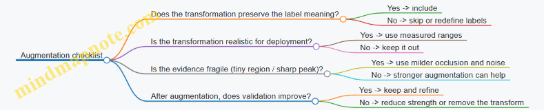
When augmentation is chosen with label safety and deployment realism in mind, it becomes a controlled tool rather than a randomizer. The goal is consistent: teach the model the variations you expect, without teaching it contradictions.
4. Feature Design and Preprocessing Pipelines
4.1 When to Use Raw Inputs Versus Engineered Features
A good rule of thumb: use raw inputs when the model can learn the useful transformations from data you can reliably collect; use engineered features when you need to control variability, reduce compute, or encode domain knowledge that the model would otherwise have to rediscover.
What “raw” really means in embedded ML
Raw inputs are the measurements in their original form (or with only basic, consistent scaling). Examples include:
- Audio waveform samples (possibly normalized).
- IMU streams of accelerometer and gyroscope readings.
- Pixel intensities from a small grayscale image.
- Sensor values sampled at a fixed rate.
Raw does not mean “no preprocessing.” In practice, you still do windowing (grouping samples into frames), basic normalization (e.g., subtract mean, divide by range), and sometimes clipping to handle outliers. The key difference is that you avoid hand-crafted transformations like FFT magnitudes, handcrafted motion statistics, or geometry-derived features.
What “engineered features” look like
Engineered features are transformations designed to make the task easier for a smaller model or a stricter runtime. Examples:
- Audio: log-mel spectrogram bins, MFCCs, or band energy ratios.
- IMU: magnitude of acceleration, jerk (difference over time), orientation estimates, or rolling statistics (mean/variance over a window).
- Vision: edge maps, downsampled histograms, or simple shape descriptors.
These features often reduce the input dimensionality and can make patterns more consistent across devices and operating conditions.
Decision criteria (with concrete examples)
1) Data volume and labeling quality
If you have lots of labeled examples that cover the real operating range, raw inputs are often a good choice because the model can learn invariances (like loudness differences in audio or small sensor biases in IMU).
Example: You’re building a keyword spotter for a controlled environment where you can record many people saying the same words. Training on raw waveform windows can work well because the model sees enough variation to learn robust representations.
If labeled data is limited or inconsistent, engineered features can help by reducing the burden on the model.
Example: You only have a few dozen recordings per class for a vibration classifier. Using band energy features (computed from each window) can improve stability because the feature extraction is deterministic and doesn’t rely on the model to learn the time-to-frequency mapping from scratch.
2) Compute budget and model size
Raw inputs can increase the input size dramatically. A 1-second audio waveform at 16 kHz is 16,000 samples; a spectrogram might be 100–300 time frames by 40–80 mel bins, which is still large but often easier to handle with a compact CNN.
Example: On a microcontroller, you might not afford a model that ingests long raw sequences. Switching to log-mel features can let you use a smaller network and still meet latency.
Engineered features can also reduce runtime work if you can compute them efficiently (or precompute them offline and store them).
Example: For IMU, computing acceleration magnitude and jerk per sample is cheap. Feeding those derived signals into a small temporal model can be faster than letting the model infer motion dynamics from three raw axes.
3) Invariance you care about
Sometimes you know which variations should not affect the prediction.
- For audio, you might want invariance to overall volume.
- For IMU, you might want invariance to device orientation.
- For vision, you might want invariance to small translations.
Engineered features can bake in invariances.
Example: If you’re detecting “tap” events, acceleration magnitude is less sensitive to which axis the tap lands on than raw x/y/z alone. A model trained on magnitude often converges faster and behaves more consistently.
Raw inputs can also achieve invariance, but only if the training data includes those variations.
4) Runtime determinism and failure modes
Engineered features can be more predictable because they have a clear mathematical definition.
Example: If you use a fixed window length and compute log-mel spectrogram bins, you know exactly what the input distribution should look like. When something goes wrong (wrong sample rate, wrong window alignment), the failure is easier to diagnose.
Raw inputs can be trickier because the model may compensate for preprocessing differences in unexpected ways.
Example: If your raw audio pipeline accidentally changes normalization or window overlap, the model might still produce outputs, but accuracy can drop silently.
5) Quantization friendliness
Quantization changes how numbers behave. Some engineered features are naturally bounded and scaled, which can make quantization easier.
Example: Log-mel features are typically normalized to a known range. Raw waveform samples might be centered around zero but can have occasional spikes; you may need clipping to keep quantized values stable.
A practical approach is to compare both pipelines under the same quantization settings and measure accuracy and runtime.
Mind map: Raw vs Engineered Features
Examples you can implement quickly
Example A: Audio classification (raw waveform vs log-mel)
Raw pipeline
- Take 1.0 s of audio at 16 kHz → 16,000 samples.
- Normalize amplitude consistently.
- Window into smaller frames only if your model requires it.
Engineered pipeline
- Compute log-mel spectrogram for each 1.0 s window.
- Normalize spectrogram values to a fixed range.
- Feed a small CNN or temporal model.
How to decide
- If your microcontroller can’t handle large input tensors, log-mel features usually win on feasibility.
- If you have abundant labeled audio covering many speakers and recording conditions, raw can be competitive.
Example B: IMU gesture recognition (raw axes vs derived signals)
Raw pipeline
- Input: sequences of (ax, ay, az) and (gx, gy, gz).
- Model learns motion patterns directly.
Engineered pipeline
- Compute acceleration magnitude: \(a = \sqrt{a_x^2 + a_y^2 + a_z^2}\).
- Compute jerk magnitude: \(j = |\Delta a / \Delta t|\) (or per-axis differences).
- Optionally compute rolling mean/variance over short subwindows.
How to decide
- If orientation varies a lot and you want axis-agnostic behavior, magnitude-based features often improve robustness.
- If you need fine-grained directionality (e.g., left vs right gestures), raw axes may preserve information that magnitude discards.
Example C: Small vision tasks (raw pixels vs edges)
Raw pipeline
- Downsample to a small grayscale image (e.g., \(96\times96\) or smaller).
- Train a compact CNN.
Engineered pipeline
- Compute edge maps (e.g., simple gradient magnitude) and feed them as input channels.
How to decide
- If lighting changes are large, edge maps can reduce sensitivity to absolute intensity.
- If the task depends on texture or color-like cues (even in grayscale), raw pixels may retain more information.
A practical baseline strategy
- Pick one pipeline that is clearly feasible on your target hardware.
- Train a model with that pipeline and measure accuracy under quantization.
- If you can afford it, run a second pipeline that differs in the “raw vs engineered” dimension.
- Choose based on the combination of accuracy, latency, and how stable the system is when preprocessing changes slightly (like window alignment or normalization).
This approach avoids arguing in the abstract. You end up with a decision grounded in what your data and hardware actually allow.
4.2 Windowing, Framing, and Overlap for Streaming Signals
Streaming signals rarely arrive in neat, fixed-size chunks. Windowing and framing turn a continuous stream into a sequence of small segments that your model can digest. The trick is choosing window length, overlap, and alignment so you capture the right temporal context without wasting compute or creating misleading duplicates.
Why windowing exists (and what it changes)
A model trained on fixed-size inputs expects each inference call to receive the same shape: for example, N samples for a 1D signal, or T×F for a spectrogram. Windowing enforces that shape by slicing the stream into segments.
But slicing also changes what the model “sees.” If your window is too short, the model may miss the full event. If it’s too long, the model may dilute the event with irrelevant context. Overlap changes how often the event appears across windows, which affects both detection timing and the number of inference calls.
Core choices: window length, hop size, and overlap
Let:
- Window length: \(L\) samples
- Hop size: \(H\) samples (how far you advance each new window)
- Overlap fraction: \(p\)
They relate by: \[ H = L(1-p) \] and the number of windows from a stream of \(S\) samples is approximately: \[ W \approx \left\lfloor \frac{S-L}{H} \right\rfloor + 1 \]
In embedded systems, \(W\) matters because it drives inference frequency and CPU load.
Mind map: windowing decisions
Windowing & Overlap Mind Map
Windowing strategies you’ll actually use
1) Disjoint windows (overlap = 0)
You take chunks back-to-back: \(H=L\). This is simple and cheap.
Example (IMU step detection):
- Sample rate: 100 Hz
- Window length: \(L=100\) samples (1 second)
- Hop size: \(H=100\)
- Overlap: 0
If a step happens at 0.1 s into the current window, the model can only report it when the window ends—up to ~1 second late. For many “detect and react” tasks, that’s too slow.
Best when: you only need coarse detection timing, or you can tolerate latency.
2) Sliding windows (overlap > 0)
You advance by a smaller hop: \(H<L\). This reduces detection latency because the event appears in multiple windows.
Example (audio keyword spotting):
- Sample rate: 16 kHz
- Window length: \(L=16000\) samples (1.0 s)
- Hop size: \(H=8000\) samples (0.5 s)
- Overlap: 50%
A keyword that occurs at time \(t\) will influence windows whose centers fall near \(t\). The system can trigger as soon as a window containing enough of the keyword is processed.
Best when: you need earlier decisions and can afford more inferences.
3) Centered windows vs trailing windows
Alignment affects latency and correctness.
- Trailing window: window ends at “now.” Good for real-time decisions.
- Centered window: window is centered on a time point. Requires future samples, so it’s not strictly causal.
Example (real-time vibration anomaly): If you use trailing windows of 2 seconds with a hop of 0.25 seconds, you can report anomalies without looking ahead. Centered windows would require buffering an extra second before you can decide.
Rule of thumb: for embedded real-time inference, prefer trailing windows unless you explicitly allow lookahead.
Choosing window length: match the event duration
A practical way to pick \(L\) is to estimate the typical duration of the signal pattern you care about.
Example (gesture classification from IMU):
- A “tap” lasts about 150–250 ms.
- Choose \(L\) around 300–400 ms to include the full motion plus a bit of context.
- If your sample rate is 100 Hz, 400 ms is 40 samples.
Then choose overlap to control update rate. If you want updates every 100 ms, hop is 10 samples, giving 75% overlap.
Choosing overlap: trade latency against compute
Higher overlap means:
- The event appears in more windows (often improving detection stability)
- More windows means more inference calls (higher power)
Example (door open detection using a vibration sensor):
- Sample rate: 200 Hz
- Window length: 1.0 s → \(L=200\)
- Hop options:
- \(H=200\) (0% overlap): decision granularity ~1.0 s
- \(H=50\) (75% overlap): decision granularity ~0.25 s
If false positives are a problem, overlap can help or hurt. It helps because you can require consistency across consecutive windows. It can hurt because noisy signals may trigger multiple overlapping windows.
Mind the “duplicate evidence” problem
Overlap creates correlated windows. If you simply threshold each window independently, you may count the same event multiple times.
Example (button press):
- Window length: 500 ms
- Hop: 50 ms
- A single press lasts 120 ms
That press will likely trigger many consecutive windows. If your application increments a counter on every positive window, you’ll overcount.
Fix: use a simple state machine or debounce.
- After a positive detection, ignore further positives for a short “cooldown” period.
- Or require \(k\) positives within the last \(m\) windows.
Implementation pattern: ring buffer framing
On embedded targets, you usually maintain a ring buffer of the last \(L\) samples. Each time you have collected \(H\) new samples, you run inference on the current window.
Example (streaming loop):
- Maintain buffer length \(L=40\) samples
- Hop \(H=10\)
- Every time 10 new samples arrive, shift in those samples, then run inference.
This avoids copying the entire stream and keeps memory predictable.
Concrete example: framing math for a 10-second stream
Assume:
- Stream length: \(S=10\) seconds
- Sample rate: 100 Hz → \(S=1000\) samples
- Window length: \(L=100\) samples (1.0 s)
- Hop: \(H=25\) samples (0.25 s)
Number of windows: \[ W \approx \left\lfloor \frac{1000-100}{25} \right\rfloor + 1 = \left\lfloor \frac{900}{25} \right\rfloor + 1 = 36 + 1 = 37 \]
So you’ll run inference 37 times over 10 seconds, i.e., 3.7 inferences per second. That’s the kind of back-of-the-envelope check that prevents “why is power so high?” surprises.
Practical checklist for windowing
- Pick \(L\) to cover the event duration plus a little context.
- Use trailing windows for real-time causality.
- Choose hop \(H\) based on acceptable detection latency and power budget.
- Expect correlated windows; add debounce or consistency logic.
- Validate with metrics that reflect streaming behavior (detection latency and false positives per unit time), not just offline accuracy.
4.3 Scaling and Quantization Friendly Preprocessing
Quantization-friendly preprocessing is mostly about being boring in the right places. If your input values look “nice” to the quantizer, you spend less time chasing accuracy drops later. The goal is simple: produce tensors whose numeric range and distribution are stable across devices, sessions, and time windows.
Why preprocessing affects quantization
Most quantization pipelines map real values to integers using a scale and a zero-point. If your preprocessing creates values with wildly different magnitudes (or lots of outliers), the scale has to cover the extremes, and the “useful” values get fewer representable steps.
A practical way to think about it: quantization resolution is roughly proportional to the chosen scale. If you double the range of your inputs, you halve the effective resolution for the values you actually care about.
Choose a target numeric range early
Before you write code, decide what range your model expects.
- For many sensor pipelines, a common target is to normalize to something like \(x \in [-1, 1]\) or \([0, 1]\).
- For audio features, log-magnitude features often work better when they’re normalized after log compression.
The key is consistency: the same preprocessing must run during training and deployment, including the same clipping or normalization logic.
Example: IMU magnitude normalization
Suppose you have accelerometer readings \(a_x, a_y, a_z\) in \(g\). A straightforward approach is to compute magnitude:
\[ m = \sqrt{a_x^2 + a_y^2 + \epsilon} \]
Then normalize using a fixed expected range. For instance, if you expect motion to stay within \([0, 2.5]\) g, clip and scale:
\[ m_{c} = \min(\max(m, 0), 2.5), \quad m_{n} = m_{c}/2.5 \]
Now \(m_n \in [0, 1]\). This keeps the quantizer from having to represent rare spikes that would otherwise stretch the scale.
Clipping: controlled outliers beat surprise outliers
Clipping is not about hiding information; it’s about deciding what “too large” means. Outliers often come from sensor glitches, motion spikes, or occasional packet corruption.
A good clipping strategy has two properties:
- It is deterministic (same rule everywhere).
- It is based on training data statistics (not guesses).
A simple method is percentile clipping. For example, compute the 99.5th percentile of absolute values on training data, then clip to that bound. If you can’t use percentiles, use a physically meaningful bound (like sensor full-scale).
Example: streaming window clipping
For a streaming signal \(s[t]\), apply preprocessing per window:
- Compute \(b = \text{clipBound}\) from training.
- Clip each sample: \(s_c[t] = \min(\max(s[t], -b), b)\).
- Normalize: \(s_n[t] = s_c[t]/b\).
This makes the input distribution stable even when a few samples are extreme.
Avoid preprocessing that depends on future data
Quantization-friendly preprocessing should not require information that arrives later than the current inference window. If you compute normalization using the entire recording, you create a mismatch between training and deployment.
Instead, prefer:
- Fixed constants derived from training.
- Per-window normalization that uses only the window’s samples.
Per-window normalization can be quantization-friendly if it doesn’t create division by tiny numbers. Add a small \(\epsilon\) and clamp the denominator.
Example: per-window standardization with safe denominator
For a window \(x\), compute mean \(\mu\) and standard deviation \(\sigma\). Use:
\[ \sigma_{s} = \max(\sigma, \sigma_{min}), \quad x’ = (x-\mu)/\sigma_{s} \]
Then optionally clip \(x’\) to \([-k, k]\) and scale to a target range. This prevents one nearly-constant window from producing huge values.
Quantization-friendly scaling rules of thumb
These rules help you avoid common “it worked in float” surprises.
- Prefer linear scaling over nonlinear scaling when possible. Nonlinear transforms can be fine, but they change the distribution in ways that are harder to predict.
- Keep the final tensor range bounded. If you can’t bound it, quantization will do it for you, usually poorly.
- Use the same rounding behavior in training and deployment. If you simulate quantization during training, match the rounding mode.
- Don’t normalize twice. A frequent mistake is applying both dataset normalization and per-window normalization, shrinking the dynamic range more than intended.
Fixed-point thinking without the headache
Even if you don’t implement fixed-point math manually, you can design preprocessing as if you will.
A helpful approach is to ensure that your preprocessing outputs values that map cleanly to integers. For example, if your runtime uses int8 with a typical scale, values near \([-1, 1]\) often quantize with good granularity.
If your preprocessing outputs values like \([-0.03, 0.07]\), the quantizer may still work, but you’re relying on a narrow range that can shift with sensor drift.
Example: scaling to match int8 expectations
If you plan to use int8 activations, a common target is to output inputs roughly in \([-1, 1]\). If your raw feature is already in \([0, 255]\) (like an 8-bit grayscale image), convert to float and scale:
\[ x_{n} = (x/255) \in [0,1] \]
Then, if your model expects centered inputs, shift:
\[ x_{c} = x_{n} - 0.5 \in [-0.5, 0.5] \]
This keeps the range bounded and predictable.
Mind map: scaling and quantization-friendly preprocessing
End-to-end example: audio feature pipeline that quantizes well
Consider a simple pipeline for keyword spotting using log-magnitude spectrogram features.
- Compute magnitude spectrogram \(S\).
- Log compression: \(L = \log(\max(S, \epsilon))\).
- Clip \(L\) to a training-derived range \([L_{min}, L_{max}]\).
- Scale to \([0,1]\): \[ F = (\text{clip}(L, L_{min}, L_{max}) - L_{min})/(L_{max}-L_{min}) \]
Why this helps: log compression reduces the effect of large magnitudes, clipping prevents rare spikes from dominating the scale, and the final \([0,1]\) range is bounded and stable.
Common pitfalls (and what to do instead)
- Pitfall: using min/max from each recording. This makes the scale vary between sessions. Use fixed bounds from training or per-window normalization with safe denominators.
- Pitfall: forgetting clipping during deployment. If you clip during training but not in firmware, the quantizer sees different ranges. Keep preprocessing code identical.
- Pitfall: normalizing after quantization simulation but not before. Decide where scaling happens in the pipeline and keep it consistent.
A quick checklist before you train
- Are final inputs bounded by design (via clipping or fixed scaling)?
- Are normalization constants computed only from training data?
- Does preprocessing use only the current window (no future samples)?
- Is the training preprocessing code identical to the firmware preprocessing logic?
- Have you checked that typical values occupy a meaningful portion of the target range?
If you can answer these, quantization becomes a predictable step rather than a mystery box.
4.4 Efficient Feature Extraction Examples for Audio and IMU
Feature extraction is where you trade raw sensor data for something a small model can use efficiently. The goal is not to “make it smarter”; it’s to make the input shape predictable, the values numerically stable, and the computation cheap enough to run in real time.
Mind map: what “efficient features” means
Audio: keyword spotting style features (spectrogram + log)
Use case: classify short audio events (e.g., “yes” vs “no”) from a microphone stream.
Step 1: Frame the signal
Take the audio stream and split it into overlapping frames. A common starting point is:
- Sample rate: 16 kHz
- Frame length: 25 ms → 400 samples
- Hop length: 10 ms → 160 samples
This yields 100 frames per second. If your model expects, say, 49 frames, you can set the inference window to 490 ms.
Why it works: the model sees local frequency patterns that change over time, while the overlap keeps the representation smooth.
Step 2: Apply a window function
Multiply each frame by a Hann window to reduce spectral leakage. In embedded code, precompute the window coefficients once and store them as fixed-point.
Example reasoning: without a window, a tone that doesn’t align with an FFT bin spreads energy across bins, which makes classification harder and more sensitive to small timing shifts.
Step 3: Compute a magnitude spectrum
Compute an FFT per frame and take magnitude. For efficiency, you can compute power directly: \[ P[k] = \Re(X[k])^2 + \Im(X[k])^2 \]
Then you can normalize by a constant factor so values stay in a predictable range.
Step 4: Convert to Mel filterbank energies
Instead of using all FFT bins, sum power into a smaller set of Mel-spaced bands (e.g., 20–40 filters). Precompute the filterbank matrix offline.
Embedded-friendly detail: implement this as a matrix-vector multiply per frame. If you use 32 filters, your output per frame is 32 numbers.
Step 5: Log scaling
Apply a log-like transform to compress dynamic range. A practical fixed-point approach is: \[ \text{feat} = \log(\max(P, \epsilon)) \]
If you want to avoid floating point, approximate log with either a lookup table or a piecewise function. The key is consistent scaling between training and inference.
Example: if you train with natural log and inference uses log10, your thresholds and calibration will drift. Pick one and stick to it.
Step 6: Stack frames into a fixed tensor
For a 490 ms window with 10 ms hop, you might get 49 frames. If your model expects \(T=49\) and \(F=32\), your input tensor is \(49 \times 32\).
Streaming note: maintain a ring buffer of raw samples. Each time you have enough samples for a new frame, compute one new feature frame and append it to a feature ring buffer.
Concrete mini-example (shapes)
- Input audio: 16,000 samples/sec
- Frame: 400 samples
- Hop: 160 samples
- Feature per frame: 32 Mel bands
- Inference window: 0.5 sec → about 50 frames
So the model input is roughly \(50 \times 32\). That’s small enough to fit typical TinyML tensor limits, and it’s stable across devices.
IMU: efficient features for motion classification (stats + derivatives)
Use case: classify gestures or detect activity using accelerometer and gyroscope.
IMU signals are already low bandwidth, so you can often get away with simpler features than audio.
Step 1: Choose a window and sampling rate
Pick a window length that matches the motion duration. For example:
- Sampling rate: 100 Hz
- Window: 1.0 sec → 100 samples
- Hop: 0.1 sec → 10 samples
Your model input might be \(100 \times C\), where \(C\) is the number of channels (e.g., ax, ay, az, gx, gy, gz).
But many embedded designs prefer feature vectors rather than raw sequences.
Step 2: Use norms to reduce sensitivity to orientation
Compute magnitude of acceleration and angular velocity: \[ |a| = \sqrt{a_x^2 + a_y^2 + a_z^2} \] \[ |\omega| = \sqrt{g_x^2 + g_y^2 + g_z^2} \]
Efficiency trick: if you want to avoid square roots, you can use squared norms \(a_x^2+a_y^2+a_z^2\) and \(g_x^2+g_y^2+g_z^2\). The model can learn with those consistently.
Reasoning: norms are less sensitive to how the device is rotated, which reduces the need for heavy preprocessing.
Step 3: Handle gravity for accelerometer features
Raw acceleration includes gravity. A common approach is to estimate gravity with a low-pass filter and subtract it: \[ a_{dyn} = a - a_{grav} \]
Then compute features from \(a_{dyn}\) rather than \(a\).
Concrete example: if you’re detecting taps, gravity dominates \(a\) during still periods. Using \(a_{dyn}\) makes the tap spike stand out.
Step 4: Compute windowed statistics
For each channel (or for norms), compute a small set of statistics over the window:
- Mean
- Standard deviation
- Min and max
- Peak-to-peak
- Energy (sum of squares)
For example, for \(a_{dyn}\) magnitude squared \(s(t)=|a_{dyn}(t)|^2\):
- \(\text{mean}(s)\)
- \(\text{std}(s)\)
- \(\text{max}(s)\)
- \(\text{energy}(s)=\sum_t s(t)\)
Why this is efficient: it turns 100 samples into, say, 4–8 numbers per signal, which reduces model size and inference time.
Step 5: Add simple temporal derivatives
Motion often shows up as changes. Compute first differences: \[ \Delta x(t) = x(t) - x(t-1) \]
Then compute the same statistics on \(\Delta\) signals. For taps, derivatives spike even if absolute values are modest.
Example: a slow tilt might change \(|a|\) gradually, but \(\Delta|a|\) stays small. A sudden gesture produces a sharp derivative peak.
Step 6: Feature vector assembly
A practical feature vector might include:
- \(|a_{dyn}|^2\): mean, std, max, energy
- \(|\omega|^2\): mean, std, max, energy
- \(\Delta|a_{dyn}|^2\): max
- \(\Delta|\omega|^2\): max
That’s 9–10 features total. A small classifier can work well with this.
Mind map: audio vs IMU feature choices

Implementation example: fixed-point friendly preprocessing checklist
- Precompute constants: FFT twiddle factors, Mel filterbank weights, Hann window.
- Use consistent scaling: match training preprocessing exactly (same normalization and log base).
- Avoid dynamic allocation: ring buffers and fixed arrays only.
- Minimize branching: clamp values with arithmetic where possible.
- Keep tensor shapes fixed: pad or choose window sizes that always produce the same \(T\).
Tiny end-to-end example: from stream to model input
Audio pipeline (per inference window):
- Collect 0.5 s of samples into a ring buffer.
- For each new hop, compute one frame’s Mel log energies.
- Maintain a feature ring buffer of \(T\) frames.
- When \(T\) frames are ready, copy into the model input tensor \(T \times F\).
IMU pipeline (per inference window):
- Collect 1.0 s of IMU samples.
- Update gravity estimate with a low-pass filter.
- Compute \(a_{dyn}\) and norms (or squared norms).
- Compute window statistics and derivative peaks.
- Pack into a fixed feature vector and run inference.
These patterns keep preprocessing predictable and cheap, which matters because the model is only half the story. The other half is making sure the input you feed it is stable, correctly scaled, and shaped exactly the way you trained it.
4.5 Implementing Preprocessing in Firmware With Fixed Point
Preprocessing is where your model either meets reality—or politely refuses it. In firmware, the goal is to reproduce the same numeric behavior you used during training, but with fixed-point math, limited RAM, and predictable timing.
Start by freezing the preprocessing contract
Before writing code, write down the exact contract your model expects:
- Input type: raw sensor units (e.g., m/s²), or already scaled integers.
- Windowing: how many samples per inference and the stride/overlap.
- Normalization: mean/scale (or min/max) applied per channel.
- Quantization mapping: how real values map to integer tensors.
A simple contract example for a 3-axis IMU classifier:
- Window length: 128 samples per axis
- Stride: 64 samples (50% overlap)
- Per-axis normalization: \(x’ = (x - \mu)/\sigma\)
- Quantization: \(q = \text{round}(x’ / s) + z\), where \(s\) is scale and \(z\) is zero-point
If any of these differ between training and firmware, accuracy drops even if the model weights are perfect.
Fixed-point basics that matter in preprocessing
Fixed-point math is not just “use integers.” You need consistent scaling.
- Choose a Q format for intermediate values, like Q15 (1 sign bit, 15 fractional bits) or Q31.
- Keep track of where you round. Rounding early can bias results; rounding late can overflow.
- Use saturation when converting to smaller integer types.
A practical rule: keep intermediate computations in a wider type (e.g., 32-bit), then narrow only at the final step that feeds the model.
Representing normalization in fixed point
Assume you trained with: \[ x’ = \frac{x - \mu}{\sigma} \] In firmware, compute: \[ x’ \approx (x - \mu) \cdot \alpha \] where \(\alpha = 1/\sigma\).
Then quantize to an integer tensor value: \[ q = \text{round}(x’ \cdot \beta) + z \] Here, \(\beta\) is the inverse of the model input scale (or equivalently, the factor that maps real \(x’\) into the quantized domain).
To avoid floating point, precompute \(\alpha\) and \(\beta\) as integers in a chosen Q format.
Example (IMU normalization):
- \(\mu = 0.05\) (in g)
- \(\sigma = 0.20\)
- Choose Q15 for \(\alpha\): \(\alpha_{Q15} = \text{round}(\frac{1}{0.20} \cdot 2^{15}) = \text{round}(5 \cdot 32768)=163840\)
If your raw sensor is already scaled to integer g-units, say \(x\) is in Q10 (meaning \(x_{real} = x / 2^{10}\)), then \((x-\mu)\) must be in a compatible scale before multiplying by \(\alpha_{Q15}\). This is where many implementations quietly go wrong.
A robust approach is to define one “working scale” for \(x\) and \(\mu\): convert both into the same Q format first, then apply \(\alpha\).
Windowing and streaming: preprocessing without copying everything
For real-time inference, you often want to avoid building a full window buffer by copying sample-by-sample.
Use a ring buffer per channel:
- Store raw samples as integers.
- When a window is ready, read contiguous segments into the model input buffer.
- If the window wraps, read two segments.
This keeps memory stable and timing predictable.
Example (ring buffer for 1D signal):
- Window length \(N=128\)
- Ring buffer length \(N\) (or larger if you need overlap)
- Stride \(S=64\)
When you advance by \(S\), you only need to update the write index and then assemble the next window from the ring.
Quantization-aware preprocessing: match training behavior
If training used per-channel normalization and then quantized inputs, firmware must do the same mapping.
Key checks:
- Mean and scale: use the exact \(\mu\) and \(\sigma\) values from training.
- Rounding mode: training frameworks often use round-to-nearest; implement the same.
- Clamping: if the model input quantization clamps to a min/max integer range, clamp before feeding.
A simple clamp example for int8 inputs:
- After computing \(q\), clamp to \([-128, 127]\).
A mind map for firmware preprocessing
Concrete firmware example: IMU preprocessing to int8 tensor
Below is a compact pattern for per-sample preprocessing. It assumes:
- Raw \(x\) is already in a fixed-point Q10 format.
- \(\mu\) is stored in the same Q10 format.
- \(\alpha\) is \(1/\sigma\) in Q15.
- The model input quantization uses scale \(s\) and zero-point \(z\) for mapping \(x’\) into int8.
// Q10 raw: x_real = x / 2^10
// Q10 mean: mu_real = mu / 2^10
// Q15 alpha: alpha_real = alpha / 2^15
// x' = (x - mu) * alpha  (result in Q25)
// Then map to int8 using input scale and zero-point.
int8_t preprocess_one(int32_t x_q10,
                       int32_t mu_q10,
                       int32_t alpha_q15,
                       int32_t inv_s_q,
                       int32_t z)
{
  int32_t diff = x_q10 - mu_q10;              // Q10
  int64_t prod = (int64_t)diff * alpha_q15;   // Q25
  int32_t xprime_q25 = (int32_t)prod;

  // Map x' to quantized: q = round(x' * inv_s) + z
  // inv_s is pre-scaled to match Q25 -> int domain.
  int64_t qwide = (int64_t)xprime_q25 * inv_s_q;
  int32_t q = (int32_t)((qwide + (1LL<<30)) >> 31) + z; // example rounding

  if (q < -128) q = -128;
  if (q > 127)  q = 127;
  return (int8_t)q;
}
The placeholder inv_s_q and shift amount depend on how you choose the Q format for the mapping step. The important part is the discipline: define scales, keep them consistent, and round once in a controlled place.
Verification: prove preprocessing matches training
You can’t eyeball correctness. Use a deterministic test:
- Pick 3 windows from real sensor logs.
- Run preprocessing in your training environment (float) and in firmware (fixed point).
- Compare the final quantized tensor values \(q\) element-by-element.
If you can’t match bit-for-bit, compare at least:
- Max absolute difference in intermediate \(x’\)
- Distribution of \(q\) values (counts per int level)
- Worst-case samples near clamping boundaries
A common failure mode is rounding differences in the normalization step. Another is using the wrong mean/scale per channel.
Practical checklist before you integrate
- Window length and stride match training exactly
- Mean/scale values are identical and per-channel if applicable
- Fixed-point Q formats are documented in comments
- Intermediate math uses 32/64-bit to prevent overflow
- Rounding and clamping happen at the same stage as training
- A small set of windows matches expected quantized tensors
When preprocessing is correct, the model becomes predictable. When it isn’t, the model behaves like it’s listening through a wall—sometimes still “working,” but never reliably.
5. Model Selection and Architecture Patterns
5.1 Selecting Models Based on Task Type and Data Shape
Choosing a model for TinyML is mostly about matching what your data looks like to what the model can efficiently compute. The goal is not to find the “best” architecture in the abstract; it’s to find one that (1) fits the input shape, (2) learns the right pattern, and (3) still runs within your latency and memory limits.
Start with a task checklist (before architecture)
- What is the output?
- Classification: one label per window (e.g., “tap” vs “no tap”).
- Detection: multiple events over time (e.g., “start/stop” segments).
- Regression: a continuous value (e.g., temperature estimate).
- Anomaly scoring: “normal vs not normal,” often with thresholds.
- How does data arrive?
- Single snapshot (one image frame).
- Sliding window stream (audio frames, IMU samples).
- Variable length (rare on microcontrollers; usually you convert it to fixed windows).
- What constraints matter most?
- Latency (must finish before the next window).
- RAM (tensor arena and buffers).
- Flash (model weights).
A practical rule: if your data is naturally windowed (audio, IMU, vibration), pick models that consume fixed-size windows. If your data is naturally images, pick models that consume fixed-size crops or resized frames.
Mind map: model choice by task and data shape
Map common data shapes to model families
1) 1D time series (IMU, vibration, ECG-like signals)
Data shape:
- Input tensor often looks like \([T, C]\) where \(T\) is window length and \(C\) is channels (e.g., 3-axis IMU).
Good starting models:
- 1D CNN with small kernels (e.g., kernel size 3 or 5) and a few layers.
- Temporal convolution stacks (often similar to 1D CNNs but with careful downsampling).
- Small RNN/GRU only if you truly need recurrence; many embedded pipelines can do well with temporal convolutions.
Example (gesture classification):
- You sample IMU at 100 Hz.
- You create windows of \(T=128\) samples (1.28 s) with overlap (e.g., 50%).
- Input shape becomes \([128, 6]\) if you use accel (3) + gyro (3).
- A compact 1D CNN can learn local motion patterns (like short spikes) without needing the model to “remember” across the entire sequence.
Why this works:
- Convolutions reuse weights across time, which is efficient.
- Downsampling reduces compute while preserving coarse temporal structure.
2) 2D images (camera crops, small grayscale frames)
Data shape: \([H, W, C]\) with fixed \(H\) and \(W\).
Good starting models:
- Small CNNs with depthwise separable convolutions or modest channel counts.
- Keep early layers simple: large kernels early tend to cost more than they help.
Example (button state from a tiny crop):
- Crop a region around the button.
- Resize to \(96\times 96\) grayscale.
- Use a small CNN that outputs one of two classes: pressed / not pressed.
Why this works:
- The model focuses on spatial edges and textures.
- Fixed input size avoids dynamic shape headaches.
3) 2D time-frequency (audio spectrograms)
Data shape: \([F, T, 1]\) where \(F\) is frequency bins and \(T\) is time frames.
Good starting models:
- 2D CNN over spectrogram patches.
- Often you can treat the spectrogram like an image: local patterns in time-frequency correspond to phonemes or keywords.
Example (keyword spotting):
- Compute a log-mel spectrogram.
- Choose a fixed patch size like \(F=40\) bins and \(T=98\) frames.
- Train a small 2D CNN to classify “keyword present” vs “background.”
Why this works:
- Convolutions capture local harmonic structures and temporal transitions.
- Fixed patch size makes streaming inference straightforward.
4) Multi-sensor inputs (fusion)
Data shape: multiple channels or multiple streams.
Two common approaches:
- Channel stacking: concatenate channels into one tensor (e.g., accel+gyro as 6 channels).
- Late fusion: run separate small models per sensor and combine scores.
Example (wearable activity):
- Use accel (3) + gyro (3) as stacked channels for a single 1D CNN.
- If one sensor is often missing, late fusion can be more robust, but it costs extra compute.
Rule of thumb:
- If sensors are synchronized and always available, channel stacking is usually simpler and cheaper.
- If sensors are optional or have different sampling rates, late fusion may reduce failure modes.
Choose model size using a “capacity fit” method
Instead of starting with a huge model and shrinking, start with a small one and grow only if needed.
- Baseline model:
- Pick the smallest architecture that can represent the task.
- Use a few layers and modest channel counts.
- Check learning behavior:
- If training accuracy is low, the model lacks capacity or preprocessing is wrong.
- If training accuracy is high but validation is low, you may need better data coverage or regularization.
- Quantization check early:
- If quantization causes a big accuracy drop, the model may be too sensitive.
Concrete example (audio):
- Baseline: a small 2D CNN with ~20–50k parameters.
- If float accuracy is good but int8 accuracy collapses, reduce reliance on very fine-grained features by adjusting preprocessing (e.g., spectrogram normalization) or using a slightly different architecture with smoother activations.
Match output format to deployment logic
Model output should align with what your firmware can do.
- Classification per window: output probabilities for each class.
- Firmware can apply a threshold and a debounce window.
- Detection over time: output per-frame scores.
- Firmware can smooth with a short moving average and require consecutive frames above threshold.
- Regression: output a scalar.
- Firmware can clamp to valid ranges and apply calibration.
Example (tap detection):
- Model outputs a probability \(p\) for “tap” per window.
- Firmware uses two thresholds: enter threshold \(\theta_{on}\) and exit threshold \(\theta_{off}\) (with \(\theta_{on} > \theta_{off}\)).
- This reduces flicker when the signal hovers near the boundary.
Quick decision examples
Example A: “Classify 2-second IMU windows into 5 gestures.”
- Data shape: 1D time series \([T, C]\).
- Task: multi-class classification.
- Start with: small 1D CNN.
- Output: softmax over 5 classes.
- Post-processing: optional smoothing across overlapping windows.
Example B: “Detect a keyword in streaming audio.”
- Data shape: 2D time-frequency patch.
- Task: classification per window, then event logic.
- Start with: small 2D CNN on log-mel spectrogram.
- Output: sigmoid for keyword vs background.
- Post-processing: hysteresis thresholding to avoid rapid toggling.
Example C: “Estimate temperature from a sensor stream.”
- Data shape: 1D time series.
- Task: regression.
- Start with: small temporal conv network.
- Output: one scalar; firmware applies calibration and clamps.
Practical constraints that affect model choice
- Fixed input sizes: choose preprocessing that yields fixed \(T\), \(H\), \(W\), and \(F\).
- Operator support: prefer common layers (conv, pooling, fully connected) that convert cleanly.
- Activation memory: deeper models can be compute-friendly but memory-heavy due to intermediate tensors.
A good selection process ends with a simple question: “If I feed one window, can the model finish inference before the next window arrives, using the memory my firmware can spare?” If the answer is no, the model family might be fine, but the size or input representation needs adjustment.
5.2 Lightweight CNNs for Images and Spectrograms
Lightweight CNNs are a practical choice when you need image or audio-like inputs on-device: they learn local patterns, reuse weights across space or time, and can be made small enough to fit tight memory and latency budgets. The trick is to design the network around the input shape and around what you can afford to compute.
What “lightweight” means in practice
A CNN is lightweight when you control three things:
- Parameter count (weights stored in flash/ROM).
- Activation footprint (intermediate tensors stored in RAM during inference).
- Compute cost (multiply-accumulate operations per inference).
A useful rule of thumb: if your model fits but crashes, it’s usually activation memory, not parameters. If it runs but misses deadlines, it’s usually compute.
Mind map: design decisions for lightweight CNNs
Architecture patterns that work well
1) “Small kernels + gradual downsampling”
Use repeated 3x3 convolutions and reduce resolution step-by-step. For images, a common pattern is:
- Conv(3x3) → Conv(3x3) → stride-2 downsample
- Repeat with increasing channels
- End with global average pooling
For spectrograms, treat time and frequency as two axes. You can downsample time more conservatively than frequency if timing matters for your classes.
Example (image classifier skeleton):
- Input: 96x96x1 (grayscale) or 96x96x3
- Block A: 3x3 conv (8 ch) → 3x3 conv (8 ch) → stride-2
- Block B: 3x3 conv (16 ch) → 3x3 conv (16 ch) → stride-2
- Block C: 3x3 conv (32 ch) → 3x3 conv (32 ch) → stride-2
- Global average pooling → dense to K classes
This structure keeps early layers cheap and pushes most compute into later layers with smaller spatial maps.
2) Depthwise separable convolutions (when channels are the bottleneck)
A standard convolution with kernel size \(k\times k\), input channels \(C_{in}\), output channels \(C_{out}\) costs roughly: \[ \text{MACs} \approx H,W,k^2,C_{in},C_{out} \] Depthwise separable conv splits it into:
- Depthwise: \(H,W,k^2,C_{in}\)
- Pointwise (1x1): \(H,W,C_{in},C_{out}\) So: \[ \text{MACs} \approx H,W,(k^2,C_{in} + C_{in},C_{out}) \] When \(C_{out}\) is not huge relative to \(C_{in}\), this can cut compute a lot.
Example (spectrogram block):
- Depthwise 3x3 conv (groups = channels)
- Pointwise 1x1 conv to mix channels
- Optional stride-2 on the time axis only (e.g., stride \((2,1)\))
This is especially handy for spectrograms because you often have a single channel input but many feature channels after the first few layers.
3) Bottlenecks with 1x1 convolutions (when you need channel mixing cheaply)
A bottleneck reduces channels before a heavier operation, then expands back. Even if you don’t use a full “residual” design, the idea is useful:
- 1x1 conv to reduce channels
- 3x3 conv on reduced channels
- 1x1 conv to restore channels
Example (tiny image model):
- Input 64x64x3
- 1x1 conv: 3 → 8
- 3x3 conv: 8 → 8
- 1x1 conv: 8 → 16
- Downsample
This reduces the cost of the 3x3 layers, which scale with \(C_{in},C_{out}\).
Spectrogram-specific choices
Spectrograms are not images in the strict sense, but CNNs treat them similarly. The key differences are in preprocessing and in how you downsample.
Choose pooling/strides that respect time
If your classes depend on when something happens (e.g., a short event), avoid aggressive time downsampling early. A safe approach is:
- Downsample frequency more than time.
- Use stride \((1,2)\) or pooling that reduces frequency first.
Use normalization that matches deployment
If you normalize spectrogram values during training (e.g., per-utterance mean/variance or fixed scaling), apply the same transformation on-device. A lightweight CNN can be accurate in training and fail in production if the input scaling differs by even a small factor.
Concrete example: a tiny CNN for spectrogram classification
Assume:
- Input spectrogram: \(T\times F\) = 64x40, single channel
- Classes: K = 12
A compact design:
- Conv 3x3, 8 channels, stride (1,1)
- Depthwise separable conv 3x3, 16 channels, stride (2,1) to reduce time gently
- Depthwise separable conv 3x3, 24 channels, stride (1,2) to reduce frequency
- Conv 1x1 to 32 channels
- Global average pooling over time and frequency
- Dense 32 → 12
Why this works:
- Early layers capture local patterns in both time and frequency.
- Strides reduce dimensions without destroying temporal resolution too quickly.
- Global average pooling avoids a large flatten layer, which would otherwise inflate activation memory.
Training details that matter for lightweight CNNs
Use augmentation that matches your sensor reality
For images:
- Small random crops and horizontal flips can help when orientation varies.
- Avoid heavy color jitter if your device input is stable and grayscale.
For spectrograms:
- Time masking (zeroing short time spans) helps robustness to missing segments.
- Frequency masking helps when some bands are unreliable.
The goal is to teach the model invariances you actually have in the field.
Match the loss to the deployment decision
If you will use a confidence threshold or a reject option, train with that in mind:
- Use a standard classification loss for logits.
- Calibrate thresholds using a held-out set that reflects your real class distribution.
This keeps the model’s output meaningful when you later decide “accept” vs “ignore.”
Debugging with simple checks
When a lightweight CNN underperforms, start with these practical checks:
- Activation sanity: confirm input shapes match exactly (especially spectrogram dimensions).
- Overfitting check: if training accuracy is low, the model is too small or preprocessing is off.
- Quantization sensitivity: if float accuracy is good but quantized accuracy drops, inspect layers with large dynamic ranges.
- Class confusion: look at which classes are mixed; often it points to preprocessing or label noise rather than architecture.
Summary
Lightweight CNNs for images and spectrograms are built by controlling downsampling, channel widths, and pooling strategy, then choosing efficient convolution variants when compute is tight. For spectrograms, downsample time carefully and keep input scaling consistent between training and deployment. If you design the network around these constraints, the model tends to be both fast and stable—without needing complicated tricks.
5.3 Small RNN and Temporal Convolution Patterns for Sequences
Sequence tasks on tiny devices usually boil down to two questions: (1) how to summarize time without storing the whole history, and (2) how to keep the compute predictable. Small RNNs and temporal convolutions answer those questions differently, so it helps to choose based on the shape of your data and the latency you can afford.
Mind map: choosing sequence patterns
Small RNN patterns: compact state, careful gates
A small RNN processes one time step at a time and carries a hidden state vector forward. For embedded inference, the key is to keep the hidden size small and the recurrence simple.
1) Vanilla RNN (baseline)
- Update: \(h_t = \tanh(W_x x_t + W_h h_{t-1} + b)\)
- Output: \(y = \text{head}(h_T)\) or \(y = \text{head}(\text{pool}(h_{1..T}))\)
This is the simplest to implement, but it often struggles with longer dependencies because \(\tanh\) can saturate. Still, it’s a useful baseline when your sequences are short and the discriminative cues are near the end.
2) GRU (common small choice) GRUs add gates that control how much of the past to keep. They typically outperform vanilla RNNs at similar hidden sizes.
- Practical rule: start with a small hidden size (e.g., 8–32 units) and measure accuracy vs. latency.
3) LSTM (usually heavier) LSTMs can work well, but they maintain both hidden and cell states, which increases memory and compute. On tiny targets, GRU often gives a better accuracy-to-cost ratio.
Streaming example: IMU gesture classification
- Input: 3-axis IMU sampled at 50 Hz
- Window: 1.0 s → 50 steps
- Model: GRU with hidden size 16
- Output: 6 gesture classes
A practical approach is to run inference continuously with a sliding window. If you can’t afford full sliding windows, you can instead buffer 50 samples, run once, then shift by a smaller stride (e.g., 10 samples). The RNN itself can be stateful within the window, but you still need a clear policy for how the hidden state resets between windows.
Best practice: define the state reset explicitly
- If windows overlap heavily, resetting state each time can waste information.
- If windows are independent events, resetting state avoids cross-event contamination.
A simple policy for embedded systems is: reset state at the start of each labeled window during training, then mirror that behavior at inference.
Temporal convolution patterns: fixed receptive fields you can count
Temporal convolutions use 1D kernels over time. They don’t carry a hidden state; instead, they build a receptive field that grows with depth and dilation.
1) Plain 1D CNN over time
- Use a stack of Conv1D layers with stride 1
- Downsample with pooling or strided conv
- End with global average pooling or flatten + dense
This works well for short windows and tasks where local patterns matter (like tremor bursts or short audio cues).
2) Dilated temporal convolution (TCN-style) Dilations expand the receptive field without increasing kernel size.
- Receptive field grows roughly with \(\sum_{l} (k_l - 1) \prod_{j<l} s_j\) for strides \(s\)
- With dilation \(d\), the effective kernel span becomes \((k-1)d + 1\)
Concrete example: keyword spotting-like sequence
- Input: log-mel features (e.g., 40 bins) sampled every 10 ms
- Window: 1.0 s → 100 frames
- Treat time as the convolution axis
A small temporal conv stack might look like:
- Conv1D (kernel 5, dilation 1)
- Conv1D (kernel 5, dilation 2)
- Conv1D (kernel 5, dilation 4)
- Global average pooling over time
- Dense to 12 classes
Even with only three layers, the receptive field covers a large portion of the window, which helps when the cue spans multiple frames.
Best practice: match receptive field to the cue duration If your discriminative event lasts about 200 ms, a receptive field much larger than that can still work, but it may force the model to learn “ignore most of the window” behavior. A good starting point is to set the receptive field to cover the typical cue length plus a small margin.
Mind map: designing a temporal conv stack
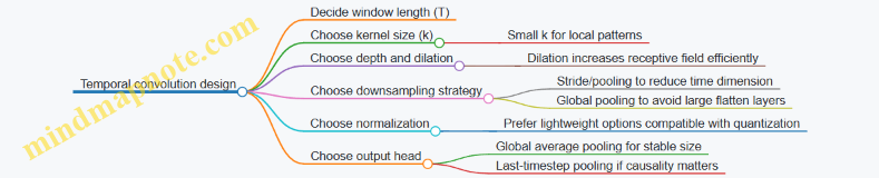
Comparing RNN vs temporal conv in embedded terms
Memory footprint
- RNN: stores hidden state (small) but may require intermediate activations depending on implementation.
- Temporal conv: stores activations for each layer over time; using global pooling can reduce the final tensor size.
Latency predictability
- RNN: processes steps sequentially, so latency scales with \(T\).
- Temporal conv: within a window, computations per layer are more uniform; latency scales with number of layers and time dimension after downsampling.
Quantization behavior
- RNNs often need careful handling of gate computations; small numerical errors can accumulate across time steps.
- Temporal convs usually quantize more straightforwardly, especially when using ReLU-like activations and avoiding fragile normalization.
Example architectures you can actually implement
Architecture A: Small GRU classifier (streaming-friendly)
- Input: \(x_t\in\mathbb{R}^d\)
- GRU hidden size: 16
- Output: take last hidden state \(h_T\)
- Head: \(y = W h_T + b\)
Architecture B: Temporal conv with global pooling (fixed-window)
- Input: \(X\in\mathbb{R}^{T\times d}\)
- Conv1D blocks with kernel 5 and dilations 1, 2, 4
- Use padding to keep time length stable (or track the reduced length)
- Global average pooling over time
- Dense head to classes
Architecture C: Hybrid (conv front-end + small RNN)
- Conv layers reduce noise and compress local patterns
- RNN processes a shorter sequence (after downsampling)
- This can reduce RNN time steps while keeping some stateful behavior
Practical training details that affect embedded success
1) Use the same windowing at training and inference If you train on fixed windows but infer on a different stride or overlap, the model sees different temporal contexts. For RNNs, that mismatch is especially noticeable because the hidden state is sensitive to sequence boundaries.
2) Choose pooling intentionally
- Last-timestep pooling: good when the decision depends on the end of the window.
- Global average pooling: good when evidence is spread across the window.
3) Keep activations quantization-friendly When you plan to quantize, prefer activations and normalization choices that behave well under integer arithmetic. If you see accuracy collapse after quantization, try simplifying the activation stack before changing the model size.
Quick decision checklist
- If you need state across time and can tolerate sequential processing: start with a small GRU.
- If you want fixed-window inference with predictable compute: start with temporal convolutions.
- If your cue spans multiple frames: ensure your receptive field (conv) or hidden state capacity (RNN) matches that span.
- If memory is tight: prefer global pooling (conv) or small hidden sizes (RNN).
These patterns are small enough to fit on constrained devices, but they’re also structured enough that you can reason about them. That’s the real advantage: you can connect a design choice (kernel size, dilation, hidden size, pooling) to what the model can “see” in time.
5.4 Keyword Spotting Style Pipelines With Practical Model Choices
Keyword spotting (KWS) is a small, practical task: detect a short word (like “start”) inside a continuous audio stream. The trick is to build a pipeline that is accurate enough while staying cheap in memory, compute, and latency. A good KWS system usually looks boring on purpose: fixed-size audio windows, consistent features, a compact model, and a simple decision rule.
The pipeline in one breath (and a few details)
- Capture audio at a fixed sample rate (commonly 8 kHz for speech).
- Frame the stream into overlapping windows (for example, 20–30 ms frames with 50% overlap, then aggregate into a fixed number of frames per inference window).
- Compute features (often log-mel spectrograms) with deterministic preprocessing.
- Run a small classifier that outputs probabilities for {keyword, other} or {keyword, silence, other}.
- Apply a decision rule that reduces false triggers (thresholding plus smoothing and a short “cooldown”).
The “style” part is choosing where to spend effort: either in the feature representation (more robust features) or in the model (more capacity). For TinyML, you typically keep features simple and let the model be small but well-structured.
Mind map: KWS pipeline components
Practical feature choices (and why they work)
Log-mel spectrograms are a common default because they compress frequency content into a small number of bins and behave reasonably under volume changes. A typical configuration is:
- Sample rate: 8,000 Hz
- FFT size: 256 (gives 16 ms at 8 kHz if you think in samples; exact mapping depends on implementation)
- Mel bins: 16 or 20
- Inference window: 1 second of audio, represented as a fixed number of frames
Normalization matters more than people expect. If you normalize per inference window (e.g., subtract mean and divide by standard deviation), you reduce sensitivity to background loudness. If you normalize globally, you must ensure the training and deployment audio levels match. For embedded systems, per-window normalization is often easier to keep consistent, but it costs a few operations; still, it’s usually cheaper than increasing model size.
Quantization-friendly preprocessing: keep scaling deterministic and avoid operations that are hard to replicate in firmware. For example, if you compute log with a floating approximation during training, you need an equivalent during inference. A safer approach is to use a fixed log approximation or compute log after applying a small floor to mel energies.
Model choice patterns that fit TinyML
KWS models often accept a 2D input: time frames × mel bins. That makes convolutional models a natural fit.
Option A: Small CNN on spectrograms
When to use: You want a straightforward pipeline and good accuracy with minimal engineering.
A typical architecture:
- 2D convolution layers with small kernels (e.g., 3×3)
- Batch normalization or layer normalization (depending on runtime support)
- ReLU-like activations
- A small pooling strategy to reduce time/frequency
- A final dense layer to produce class logits
Why it’s practical: CNNs reuse weights across time and frequency, which helps when you keep the model small.
Example input contract:
- Input:
[1, T, M]whereTis number of time frames in the inference window andMis mel bins. - Output:
[2]for {keyword, other}.
Option B: Depthwise-separable CNN (mobile-friendly)
When to use: You care about compute per inference.
Depthwise-separable convolutions split spatial filtering into depthwise and pointwise steps. This reduces multiply-accumulate counts while keeping the model expressive.
Practical rule: If your CNN is too slow, replace standard convolutions with depthwise-separable ones before you start changing the feature pipeline.
Option C: Tiny CRNN (convolution + recurrent)
When to use: You want temporal context without making the model huge.
A small recurrent layer (GRU or simple RNN) can capture longer patterns than a purely convolutional model. For TinyML, keep the recurrent hidden size small.
Tradeoff: Recurrent layers can be harder to optimize and may increase latency variance depending on the runtime.
Option D: Fully convolutional with global pooling
When to use: You want to avoid dense layers and reduce memory.
Global average pooling over time and frequency can replace a large flatten-and-dense stage. That often improves portability because it reduces the number of parameters.
A concrete “keyword vs other” example
Assume:
- Keyword: “start”
- Classes: keyword vs other
- Inference window: 1.0 s audio
- Hop: 0.1 s (so you run inference every 100 ms)
Decision rule that behaves well in practice:
- Compute probability (p_k) for keyword.
- Smooth it with a short moving average over the last 3 inferences: \[ \bar{p}_k(t)=\frac{p_k(t)+p_k(t-1)+p_k(t-2)}{3} \]
- Trigger if \(\bar{p}_k(t) > \tau\) and enforce a cooldown of 0.5 s.
This reduces single-window spikes from noise. The cooldown prevents repeated triggers while the user is still speaking.
Mind map: model selection criteria
Example model configurations (practical, not theoretical)
Below are “starter” configurations you can adapt. The exact numbers depend on your runtime and conversion tool, but these are typical sizes.
- Small CNN baseline
- Input:
T=98frames (for a 1 s window with 10 ms hop),M=16mel bins - Conv blocks: 3 blocks, channels like 8 → 16 → 24
- Pooling: reduce time by 2× in early blocks
- Head: global average pooling + dense to 2 classes
- Depthwise-separable CNN
- Same input
- Replace each conv block with depthwise-separable conv
- Keep channels slightly lower (e.g., 8 → 12 → 16)
- Head: global average pooling + dense
- CRNN-lite
- Conv front-end: 2 blocks to reduce frequency
- Recurrent: GRU with small hidden size (e.g., 16)
- Head: take last time step or average over time
How to compare fairly: keep the feature pipeline identical, train with the same splits, and evaluate using the same decision rule and cooldown. Otherwise you end up comparing the post-processing more than the model.
Training targets that match the embedded decision rule
If you plan to threshold probabilities, train with a loss that produces calibrated-ish outputs. In practice, cross-entropy works, but you should also ensure your dataset includes “hard other” examples: similar-sounding words, background speech, and quiet noise. Otherwise the model learns an easy boundary and your threshold becomes fragile.
A simple but effective dataset practice:
- Balance keyword examples across different volumes.
- Include non-keyword clips that contain speech-like patterns.
- Keep the same preprocessing (windowing and mel settings) used at inference.
End-to-end example flow (from audio to trigger)
- Maintain a rolling buffer of 1.0 s audio.
- Every 100 ms, compute mel features for the newest 1.0 s window.
- Quantize features using the same scaling constants used in training.
- Run inference to get \(p_k\).
- Smooth \(p_k\) and apply threshold \(\tau\).
- If triggered, record the event time and start cooldown.
This structure keeps the system predictable: fixed compute per step, fixed memory allocations, and a decision rule that you can reason about.
Quick checklist for a working KWS pipeline
- Feature extraction is deterministic and matches training.
- Model input shape is fixed and validated in firmware.
- Post-processing includes smoothing and cooldown.
- Evaluation reports both false accepts and false rejects.
- You measure end-to-end latency, not just model inference time.
Keyword spotting is a small system with many small parts. When those parts agree—features, model, and decision rule—the result is usually accurate and stable without needing anything complicated.
5.5 Baseline Models and How to Compare Fairly
A baseline is not “the simplest model.” It’s the simplest model that answers a specific question: Is the improvement coming from better modeling, better preprocessing, or better evaluation? If you compare models without controlling those factors, you end up measuring your pipeline’s quirks instead of the model.
What to baseline (and what not to)
Start by listing the decisions that can change results:
- Input representation (raw vs windowed vs normalized)
- Preprocessing (filtering, scaling, spectrogram settings)
- Model capacity (number of layers, channels, hidden units)
- Training recipe (optimizer, learning rate schedule, epochs)
- Quantization path (float-only evaluation vs quantization-aware evaluation)
- Decision rule (argmax vs threshold vs reject option)
A fair comparison keeps everything constant except the variable you want to study.
Baseline categories that cover most TinyML work
Use a small set of baselines that bracket the problem:
- Heuristic baseline: no learning, rules derived from the data.
- Linear baseline: learning with minimal capacity.
- Small neural baseline: a compact network that matches your deployment constraints.
- “Same architecture, different training” baseline: identical model, different preprocessing or quantization handling.
This mix helps you separate “the data is easy” from “the model is learning the right thing.”
Mind map: baseline design and comparison
Step-by-step: building a baseline suite
1) Lock the data pipeline
Pick one canonical pipeline and reuse it for every baseline.
- For streaming signals, fix window length and overlap.
- For normalization, compute statistics on the training split only, then apply them to validation/test.
- For audio spectrograms, fix FFT size, hop length, mel bins, and log scaling.
Example (IMU gesture):
- Window length: 1.0 s
- Overlap: 50%
- Features: per-axis mean and standard deviation over the window
- Normalization: z-score using training-set mean/std
Every baseline uses the same windows and the same normalized features.
2) Choose decision rules up front
If you use thresholds, decide how they’re set.
- Argmax is simple but hides “I’m not sure” behavior.
- Threshold + reject is useful for real-time systems that must avoid false triggers.
Fair comparison rule: use the same threshold selection method for all models.
Example (keyword spotting):
- Compute validation scores.
- Choose a threshold that targets a fixed false accept rate.
- Apply that threshold unchanged to test for every baseline.
3) Define metrics that match the product behavior
Accuracy alone can be misleading when classes are imbalanced or when timing matters.
Use at least:
- Primary metric: e.g., macro F1 for imbalanced classes
- Operational metric: e.g., false positives per minute
- Calibration/threshold metric: e.g., rejection rate at a target false accept
Example (equipment vibration):
- Positive class is rare.
- Report: recall at a fixed false alarm rate, not just overall accuracy.
Baseline examples you can implement quickly
Heuristic baseline: energy threshold
For many sensor tasks, the first useful baseline is “does something exceed a level?”
- Compute signal energy in each window: \(E = \sum_t x_t^2\)
- Predict class 1 if \(E > \tau\), else class 0
Example (tap detection):
- Use accelerometer magnitude \(|a|\)
- Set \(\tau\) by scanning validation windows to hit a target false positive rate
This baseline is valuable because it tells you whether the task is mostly separable by amplitude patterns.
Linear baseline: logistic regression on engineered features
If you already have features (means, stds, spectral band energies), a linear model is a strong sanity check.
- Input: engineered feature vector \(\phi(x)\)
- Model: \(p(y=1|x)=\sigma(w^T\phi(x)+b)\)
Example (IMU gestures):
- Features: mean, std, and max of each axis (plus magnitude stats)
- Compare against your neural model to see whether the neural net is learning non-linear structure or just reweighting features.
Small neural baseline: tiny CNN or MLP
Pick a model that fits your deployment budget and uses the same input representation as the other baselines.
- For spectrogram-like inputs: a small 2D CNN with a few conv layers
- For feature vectors: a small MLP with dropout disabled during evaluation
Example (audio):
- Input: \(T\times F\) log-mel spectrogram
- Model: 2 conv blocks + global average pooling + linear classifier
- Keep the same preprocessing as the heuristic and linear baselines
Same-architecture variants: isolate one change
Once you have a small neural baseline, create controlled variants:
- Variant A: float training, float evaluation
- Variant B: float training, quantized evaluation
- Variant C: quantization-aware training, quantized evaluation
Fair comparison rule: only one variant changes at a time.
A practical fairness checklist
Before you trust a comparison, verify:
- Same splits: identical train/val/test windows
- Same windowing: same overlap and alignment
- Same preprocessing: same parameters and normalization method
- Same threshold policy: same selection on validation, same application on test
- Same evaluation mode: either all float or all quantized
- Same post-processing: smoothing, majority vote, or debounce logic
A common mistake is applying different normalization per model. Even if the model is different, the data pipeline should be identical.
Reporting results in a way that helps decisions
For each baseline, report a compact set of numbers:
- Metric: e.g., macro F1 or recall@false-alarm-rate
- Threshold behavior: reject rate or false accepts at the chosen operating point
- Compute: latency per inference and peak memory (or arena size)
Example reporting format (for a keyword task):
- Heuristic energy threshold: recall 0.62, false accepts 0.8/min
- Linear model: recall 0.71, false accepts 0.6/min
- Small CNN: recall 0.78, false accepts 0.5/min
- Same-arch QAT: recall 0.76, false accepts 0.5/min
Notice how the last two lines answer a specific question: whether quantization-aware training helps under the quantized evaluation path.
Interpreting baseline gaps
When a neural model beats a linear model, it suggests non-linear structure in the input representation. When the heuristic is close to the neural model, the task may be mostly separable by simple statistics, and improvements should focus on preprocessing or decision rules. When float accuracy is high but quantized accuracy collapses, the issue is often quantization sensitivity rather than model capacity.
Baselines are your microscope. They don’t just tell you what works; they show you why the comparison is meaningful.
6. Training Workflows and Evaluation for TinyML
6.1 Reproducible Training Setup and Experiment Tracking
Reproducibility is less about magic and more about making the training run a well-specified recipe. If you can’t explain why run A beats run B in one page, you probably can’t reproduce it either.
What “reproducible” means in practice
A training run is reproducible when you can regenerate the same results (or extremely close results) given the same code and data. In TinyML workflows, “close” matters because quantization and preprocessing can amplify tiny differences.
Key sources of variation:
- Data order: shuffling without a fixed seed changes batches.
- Preprocessing randomness: augmentations that use random parameters.
- Floating-point nondeterminism: some GPU kernels and parallel reductions can vary.
- Environment drift: different library versions change numerics.
- Silent config changes: thresholds, window sizes, and label mapping tweaks.
Mind map: reproducibility checklist
Reproducible Training Setup (Mind Map)
A concrete setup: “one run = one folder = one truth”
Create a run directory that stores everything needed to re-run training. The naming should include a human-readable tag and a unique identifier.
Example run folder structure:
runs/2026-03-25_imu_gesture_seed42_run7/config.yamltrain.logmetrics.csvcheckpoints/epoch_XX.ptartifacts/label_map.jsonnormalization_stats.jsondataset_manifest.json
This makes it easy to answer: “Which exact preprocessing and label mapping produced this checkpoint?”
Capturing configuration without relying on memory
Use a single config file that includes every training-relevant parameter. Avoid scattering values across scripts.
Minimum config fields:
- dataset paths and dataset manifest identifier
- label mapping version
- preprocessing parameters (window length, overlap, scaling method)
- augmentation parameters and whether they are enabled
- model hyperparameters (input shape, number of channels, layer sizes)
- optimizer settings (learning rate, weight decay)
- training settings (batch size, epochs, gradient accumulation)
- evaluation settings (batch size, metrics, thresholding rules)
A small but effective rule: if a value affects the computation graph or the input tensors, it belongs in the config.
Seeding: do it everywhere randomness appears
Set a global seed and ensure it reaches every component that can sample randomness.
Common places to seed:
- Python
random - NumPy
- the deep learning framework
- data loader workers (each worker needs a deterministic seed derived from the base seed)
- augmentation transforms
Example (PyTorch-style pseudocode):
import random, numpy as np
import torch

def seed_everything(seed: int):
    random.seed(seed)
    np.random.seed(seed)
    torch.manual_seed(seed)
    torch.cuda.manual_seed_all(seed)
    torch.backends.cudnn.deterministic = True
    torch.backends.cudnn.benchmark = False
If you use multiple workers, also seed worker processes deterministically. The goal is that the same sample index always produces the same augmented tensor under the same seed.
Dataset manifest: stop arguing about what “the dataset” is
A dataset manifest is a record of what files were used and how they map to labels. It should include:
- list of data files (or shards)
- file hashes (or at least sizes + modification times)
- label mapping version
- preprocessing stats version (if computed offline)
Example manifest fields:
dataset_id: a stable identifierfiles: array of{path, sha256, num_samples}label_map_sha256preprocess_stats_sha256
This prevents the classic issue where you retrain after a data copy and accidentally change one file.
Experiment tracking: log what you’ll need later
Tracking isn’t just “accuracy over time.” For reproducibility, you need logs that let you reconstruct decisions.
Log at least:
- training loss and validation metrics per epoch
- learning rate per epoch (or per step)
- batch size and effective batch size
- number of training samples and class distribution
- best checkpoint criterion (e.g., highest validation F1 at fixed threshold)
- evaluation threshold and how it was chosen
A practical approach is to write a metrics.csv with one row per epoch:
epochtrain_lossval_accuracyval_f1val_precisionval_recalllrbest_flag
Mind map: what to track (and why)
Experiment Tracking (Mind Map)
Example: tracking a thresholded metric correctly
Suppose your deployment uses a confidence threshold to decide “reject” vs “accept.” If you compute accuracy without applying the threshold, you’ll pick a checkpoint that looks good in training but behaves poorly on-device.
A clean method:
- During validation, compute logits/probabilities.
- Apply the same threshold used for deployment.
- Track the metric under that threshold.
If you tune the threshold, store it in the run folder and log how it was chosen (fixed value vs searched on validation).
Example: a minimal “run record” template
This record is small enough to read and detailed enough to reproduce.
Common failure modes (and quick fixes)
- Changing label mapping: store
label_map.jsonand hash it. - Augmentation mismatch: log augmentation parameters and whether it’s enabled for train only.
- Different normalization stats: save the exact stats used for scaling.
- Best checkpoint ambiguity: explicitly define the selection rule and log it.
- Non-deterministic data loading: seed worker processes and keep shuffling deterministic.
A simple workflow that stays manageable
- Create a config file for the run.
- Generate a dataset manifest and preprocessing stats artifacts.
- Seed everything deterministically.
- Train while logging metrics, learning rate, and best checkpoint criteria.
- Save a run record that points to every artifact.
Do this once, and future experiments become comparisons instead of detective work.
6.2 Loss Functions, Metrics, and Thresholding for Deployment
Training a model is only half the job; the other half is deciding what the model should mean when it runs on a device. Loss functions shape what the model learns, metrics tell you whether it learned the right thing, and thresholding turns probabilities (or scores) into actual decisions under real constraints.
Loss functions: matching the learning signal to the decision
Classification losses
For single-label classification (one class per window), common choices are:
- Cross-entropy (CE): Good default when classes are mutually exclusive.
- Example: keyword spotting with classes
{silence, yes, no, unknown}. CE encourages the correct class to have the highest logit.
- Example: keyword spotting with classes
- Label smoothing: Slightly softens targets.
- Example: if “yes” labels sometimes include borderline audio, smoothing prevents the model from becoming overconfident on ambiguous windows.
For multi-label classification (multiple tags can be true), use:
- Binary cross-entropy (BCE) with sigmoid outputs.
- Example: vibration monitoring where both
{bearing_fault}and{imbalance}could appear in the same time window.
- Example: vibration monitoring where both
Imbalanced data losses
When “silence” dominates, plain CE can produce a model that is technically accurate but practically useless.
- Weighted cross-entropy: Increase penalty for rare classes.
- Example: if “alarm” appears 1% of windows, weight its CE term higher so the model cannot ignore it.
- Focal loss: Down-weights easy examples and focuses learning on hard ones.
- Example: in keyword spotting, many windows are clearly silence; focal loss helps the model learn the tricky boundary between “silence” and “keyword.”
Regression losses (when you predict a value)
If you predict a continuous quantity (e.g., temperature, angle, or event timing), use:
- Mean squared error (MSE) for smooth penalties.
- Mean absolute error (MAE) when outliers are common.
- Example: IMU-based tilt estimation where occasional sensor spikes should not dominate training.
Metrics: measuring what you will actually deploy
Accuracy is rarely the whole story. Deployment cares about errors that trigger actions.
Confusion-matrix-derived metrics
For binary decisions (event vs no event), define:
- Precision: among predicted events, how many were correct.
- Recall: among true events, how many were detected.
- F1 score: harmonic mean of precision and recall.
A useful mental model: precision controls false alarms; recall controls missed detections. If your device wakes the system on “event,” false alarms waste power, while missed detections break functionality.
Metrics for multi-class
For single-label multi-class, consider:
- Macro-averaged F1: treats each class equally, which is helpful when rare classes matter.
- Per-class recall: often more actionable than a single averaged number.
Metrics for ranking scores
If your model outputs a score that you threshold later, you can evaluate ranking behavior:
- ROC-AUC: shows tradeoff across thresholds.
- Precision-Recall curve: more informative when the positive class is rare.
Thresholding: turning scores into decisions
Most embedded pipelines do something like:
- Compute a score \(s \in [0,1]\) (often after sigmoid/softmax).
- Compare to a threshold \(\tau\).
- Trigger an action if \(s \ge \tau\).
The threshold is not a cosmetic detail; it is the knob that aligns model behavior with system requirements.
Choosing a threshold with a deployment objective
Suppose you want to minimize false alarms while keeping recall above a target. A practical approach:
- Sweep \(\tau\) over a grid.
- For each \(\tau\), compute recall and false positive rate (or precision).
- Pick the smallest \(\tau\) that meets recall, or the largest \(\tau\) that keeps false alarms under a limit.
This is often more stable than picking the threshold that maximizes F1, because F1 treats precision and recall as equally important, which rarely matches real systems.
Example: keyword spotting with a wake word
Assume a model outputs \(p(\text{keyword})\). You evaluate on a validation set and get these approximate results:
- At \(\tau=0.30\): recall \(=0.95\), false alarms \(=120\) per hour.
- At \(\tau=0.55\): recall \(=0.90\), false alarms \(=35\) per hour.
- At \(\tau=0.70\): recall \(=0.82\), false alarms \(=10\) per hour.
If your product requirement is “recall at least 0.88 and false alarms below 40 per hour,” you choose \(\tau=0.55\). Notice how the “best” threshold depends on the system’s tolerance, not on the model’s raw accuracy.
Example: multi-label vibration tags
For multi-label outputs, you typically use one threshold per label:
- \(\tau_{bearing}\) for
bearing_fault - \(\tau_{imbalance}\) for
imbalance
Why separate thresholds? Because each label has different prevalence and different confusion patterns. A single global threshold can over-trigger one label while under-triggering another.
Hysteresis and temporal smoothing (simple but effective)
Single-window thresholding can be noisy. A common embedded-friendly improvement is to require persistence:
- Trigger only if \(s \ge \tau\) for N consecutive windows.
- Or trigger on rising edge and reset only after \(s \lt \tau_{off}\) (hysteresis).
This reduces flicker without changing the model. It also makes behavior easier to reason about during testing.
Mind maps
Loss, Metrics, Thresholding Mind Map
Practical checklist for deployment-ready thresholding
- Pick the threshold using the same windowing and preprocessing as deployment. If your validation windows differ, the threshold will drift.
- Optimize for the system objective, not for a generic score. “Recall above X” or “false alarms below Y” beats “maximize F1” in many real pipelines.
- Use per-class thresholds for multi-label tasks. Each label has its own error profile.
- Add simple temporal rules if you see flicker. Persistence or hysteresis often beats retraining when the model is already good.
- Re-check thresholds after quantization. Quantization can shift score distributions, so the threshold may need adjustment.
Tiny example: threshold sweep in plain terms
Let \(s_i\) be the predicted score for window \(i\), and \(y_i \in {0,1}\) be the label. For each candidate \(\tau\):
- Predict \[ \hat{y}_i = \mathbb{1}[s_i \ge \tau] \]
- Compute recall and false positive rate from counts in the confusion matrix.
Then choose \(\tau\) according to your constraint. This is simple, deterministic, and easy to reproduce—exactly what you want when the device is the final judge.
6.3 Handling Class Imbalance With Concrete Examples
Class imbalance happens when one label appears far more often than others. On embedded inference, that imbalance can quietly turn into a system that “works” on paper while failing the exact cases you care about. The goal here is to make the training objective and the evaluation procedure match your real-world priorities.
What imbalance looks like in practice
Imagine a keyword spotting dataset with three labels:
yes: 50,000 clipsno: 5,000 clipssilence: 200,000 clips
Even if your model has decent overall accuracy, it can learn to treat most audio as silence because that label dominates. The fix is not just “use more data,” because collecting rare events is expensive and sometimes impossible.
Mind map: imbalance causes and fixes
Step 1: Choose the right metric before changing training
If you only track accuracy, imbalance can hide failure. For deployment, you usually care about:
- Recall for rare “positive” events (misses are costly)
- Precision for those events (false alarms are costly)
A practical approach is to compute per-class precision and recall and then decide which class is allowed to be “imperfect” and which is not.
Concrete example:
- For
yeskeyword detection, suppose missingyesis worse than a false alarm. - You would prioritize recall for
yesand accept lower precision, then use a threshold to control false alarms.
Step 2: Class-weighted loss (easy to implement, often effective)
Most training pipelines use cross-entropy loss. With class weights, the loss for each example is scaled by a factor that is larger for rare classes.
Let the dataset contain counts \(n_c\) for class \(c\). A common choice is: \[ w_c = \frac{1}{n_c} \]
In practice, you often normalize weights so their average is 1 to keep the overall loss scale stable.
Concrete example (keyword spotting): Counts:
yes: 50,000no: 5,000silence: 200,000
Raw inverse weights:
yes: 1/50,000no: 1/5,000silence: 1/200,000
Relative to silence, no gets \( (1/5,000) / (1/200,000) = 40 \times \) more weight, and yes gets \( (1/50,000) / (1/200,000) = 4 \times \) more weight.
What to watch:
- If you over-weight rare classes, the model may start predicting them too often.
- That’s not a bug; it means your decision threshold needs to be tuned, or your weights need to be less aggressive.
Step 3: Resampling (when you want the model to “see” balance)
Resampling changes how often examples are drawn during training.
- Oversampling rare classes: repeat them more often.
- Undersampling frequent classes: drop some frequent examples.
Concrete example (IMU anomaly detection): Suppose you have:
normal: 98,000 windowsanomaly: 2,000 windows
If you oversample anomaly so both classes appear equally often per epoch, the model gets more gradient signal from anomalies.
Simple rule of thumb:
- Oversampling is usually safer than undersampling when you can afford training time.
- Undersampling can remove useful variety from the normal class, especially if normal behavior has multiple modes.
What to watch:
- Oversampling can lead to overfitting on the repeated rare examples.
- Mitigate by using data augmentation for the rare class (for time series, small jitter, scaling, or window shifts that preserve the label).
Step 4: Focal loss (focus on hard examples)
Class weighting and resampling treat all examples of a class similarly. Focal loss instead reduces the contribution of easy examples by scaling the loss based on how confident the model already is.
A typical focal loss form for binary classification is: \[ \text{FL}(p_t) = -\alpha (1 - p_t)^{\gamma} \log(p_t) \] where \(p_t\) is the model probability for the true class.
Concrete example (rare event with many easy negatives): In many sensor tasks, most negative windows are clearly negative. The model quickly learns them, and training time gets wasted. Focal loss reduces the gradient from those easy negatives, letting the model spend more effort on borderline cases.
What to watch:
- If \(\gamma\) is too high, training can become unstable or overly focused on a small set of hard samples.
- Start with moderate values and verify with per-class recall.
Step 5: Decision threshold tuning (often the missing piece)
Even with balanced training, the final decision depends on thresholds.
Concrete example (binary “event vs no event”):
You train a model that outputs a probability \(\hat{p}\) for event.
- Default threshold: \(\hat{p} \ge 0.5\)
- But in imbalanced settings, \(0.5\) is rarely optimal.
Instead, compute precision and recall on a validation set and choose a threshold that meets your target.
Practical workflow:
- Sweep thresholds from 0.05 to 0.95.
- For each threshold, record precision and recall.
- Pick the threshold that satisfies your constraint, such as “recall at least 0.9.”
This is especially important when you used class weights or focal loss, because those change the effective calibration of probabilities.
Step 6: Build balanced evaluation sets without breaking realism
You want evaluation that reflects deployment costs, not just dataset proportions.
Concrete example (two evaluation modes):
- Realistic set: uses the natural frequency of events (e.g., 1% anomalies).
- Balanced set: forces equal counts per class to measure how well the model can separate classes.
A model can look great on a balanced set but still be unusable if false alarms are too frequent in the realistic set. Reporting both prevents that mismatch.
Step 7: A worked mini-case: choosing between methods
Suppose you train a 3-class classifier for yes, no, and silence.
Initial results (validation):
silencerecall: 0.98yesrecall: 0.55norecall: 0.30- Macro F1: low
You try class-weighted loss with weights based on inverse counts.
yesrecall improves to 0.72norecall improves to 0.55- But precision for
nodrops (more false alarms)
Next, you tune the decision threshold for no (or use a “reject” option when confidence is low).
noprecision recovers- Overall macro F1 improves
Reasoning summary:
- Loss reweighting fixed the learning imbalance.
- Threshold tuning fixed the decision imbalance.
Common pitfalls (and what to do instead)
- Using accuracy as the only metric: it can stay high while rare classes fail.
- Over-weighting without threshold tuning: the model may become too eager to predict rare classes.
- Resampling that removes normal diversity: undersampling can erase important normal patterns.
- Evaluating on the training distribution only: you need validation that matches deployment costs.
Quick checklist for your next training run
- Compute per-class precision/recall and confusion matrix.
- Decide which class misses are most costly.
- Try class-weighted loss first (simple and effective).
- If negatives dominate, consider focal loss.
- Tune thresholds using a validation set with the right cost profile.
- Report both realistic and balanced evaluation views.
6.4 Evaluating Accuracy Under Quantization Aware Conditions
Quantization-aware evaluation answers a simple question: “How wrong will the model be when it runs with the exact numeric rules we plan to deploy?” If you only test float accuracy, you’re measuring a version that your device will never execute. This section shows a practical way to evaluate accuracy under quantization-aware conditions, with mind maps and concrete examples.
What “quantization-aware conditions” means
In practice, you evaluate accuracy under conditions that match deployment:
- Same preprocessing: scaling, clipping, and normalization must match the firmware pipeline.
- Same quantization scheme: per-tensor vs per-channel, symmetric vs asymmetric, and the chosen bit width.
- Same runtime behavior: rounding mode, saturation, and operator implementation details.
- Same input range handling: whether inputs are clipped to min/max before quantization.
A useful mental model is: float evaluation measures “model quality,” while quantization-aware evaluation measures “model quality after numeric translation.”
Mind map: evaluation pipeline
Step-by-step evaluation method
1) Start from a fixed test set
Use a held-out test set that you never touched during training or calibration. For streaming tasks, keep the same windowing and overlap used in deployment.
Example: For keyword spotting, if you use 1-second windows with 50% overlap, evaluate on the same framing. A model that looks good on isolated clips can fail when windows shift by 0.5 seconds.
2) Freeze preprocessing and quantization contracts
Before measuring accuracy, confirm these contracts match:
- Input tensor shape and dtype: e.g.,
1 x 96 x 64spectrogram frames. - Normalization: if firmware does
x = (x - mean) / scale, the evaluation must do the same. - Quantization parameters: the scale and zero-point used for input and activations.
A common mistake is evaluating quantized inference with float preprocessing. It’s like testing a bike with the brakes removed: the numbers look fast, but they don’t represent reality.
3) Run three evaluations, not one
Do these runs on the same test set:
- Float baseline: model in float with float preprocessing.
- Quantized simulation: quantized model executed in a quantization-aware simulator (or exported quantized graph) using the same preprocessing.
- Deployment-like integer run: if possible, run the exported model with the same runtime (or as close as you can).
If (2) and (3) differ, the gap is runtime-specific. If (1) and (2) differ, the gap is numeric translation.
4) Use metrics that reflect deployment decisions
Accuracy alone can hide decision problems. For classification with thresholds, evaluate both:
- Top-1 / argmax accuracy
- Thresholded metrics (precision, recall, false reject/false accept)
Example: Suppose you deploy keyword spotting with a confidence threshold. A quantized model might keep the correct class as argmax but shift confidence downward, increasing false rejects.
Example: classification with thresholding
Assume a 4-class classifier with a “reject” option. Deployment uses:
- Compute logits (z)
- Apply softmax to get probabilities (p)
- If (max(p) < T), output “reject”
In quantized inference, you may not compute softmax in float. Instead, you might compare quantized scores directly or use an integer-friendly approximation.
To evaluate correctly:
- Compute the same decision rule in evaluation.
- Sweep threshold (T) using the quantized outputs.
- Report metrics at the chosen (T), not just at the float-tuned (T).
A tiny shift in score calibration can move many samples across the threshold. That’s why you evaluate the decision rule, not only the predicted label.
Mind map: diagnosing accuracy loss
Practical checks that catch common issues
Check A: “Quantization sanity” on a small batch
Before full evaluation, run a small batch (e.g., 100 samples) and verify:
- Input quantized values are not all the same (e.g., all zeros).
- Activations are not saturating constantly.
- The predicted class distribution is plausible.
If everything saturates, accuracy will be poor no matter how good the float model is.
Check B: Compare score distributions
For each class, compare:
- Float logits (or probabilities)
- Quantized logits (or integer scores)
Look for systematic shifts: quantization often compresses dynamic range, which can reduce separation between classes. If separation shrinks, thresholding becomes more sensitive.
Check C: Per-layer sensitivity (lightweight version)
You don’t need to instrument every layer. A practical approach is:
- Quantize the whole model.
- Then selectively keep one layer in float while quantizing the rest.
- Measure accuracy change.
The layers that cause the biggest accuracy recovery when kept in float are your numeric trouble spots.
Example: time-series model (IMU) and range calibration
Consider an IMU gesture classifier using a sliding window of accelerometer magnitude. Firmware computes magnitude and then scales to a fixed range before quantization.
Evaluation steps:
- Use the same windowing and magnitude computation.
- Ensure the evaluation uses the same scaling and clipping.
- Calibrate quantization ranges using a representative subset that includes both quiet and high-motion gestures.
If calibration ranges are too narrow, high-motion samples clip heavily. Quantization-aware evaluation will show it as a class-specific drop, often for gestures with larger amplitude.
Reporting results clearly
When you write the evaluation results, include at least:
- Float accuracy (baseline)
- Quantized simulation accuracy
- Deployment-like integer accuracy (if available)
- Metric type (argmax vs thresholded)
- Threshold value used (if applicable)
- Notes on preprocessing match (especially clipping and scaling)
A compact summary might look like:
- Float: 92.3% top-1
- Quantized sim: 89.1% top-1
- Integer runtime: 88.7% top-1
- With threshold (T=0.65): precision/recall reported separately
This makes it clear whether the loss comes from numeric translation, runtime differences, or decision logic.
Mind map: what to include in the evaluation report
Closing note
Quantization-aware evaluation is mostly about discipline: match the numeric contracts, run the same decision logic, and measure with the same metrics your firmware actually uses. Once you do that, the accuracy numbers stop being mysterious and start being actionable.
6.5 Creating an On Device Test Harness for Verification
An on-device test harness answers a simple question: “Does the firmware behave the way the model expects, under the same timing and memory constraints as production?” The trick is to test the interfaces (inputs, preprocessing, tensor shapes, thresholds) and the behavior (timing, error handling, determinism), not just the final accuracy.
What to test (and what to ignore)
Focus on three layers:
- Input contract: the exact bytes or numeric values that reach the model after preprocessing.
- Execution contract: tensor shapes, quantization parameters, operator support, and memory arena sizing.
- Decision contract: how logits/probabilities map to labels, including reject/unknown behavior.
Ignore for now: training quality, dataset bias, and “it works on my laptop” comparisons. The harness is for firmware verification.
Mind map: harness scope and components
Harness architecture: a test mode, not a separate program
A practical pattern is to compile the same firmware image with a test mode flag. In test mode, the device:
- reads test vectors from flash (or streams them over a debug interface),
- runs preprocessing + inference,
- compares outputs to expected results,
- prints a compact report.
This avoids “works in the test app, fails in production” mismatches.
Step 1: Define golden vectors
Golden vectors are fixed inputs with known expected outputs. Use them to verify the full pipeline deterministically.
For time series (IMU/audio features):
- Choose a few windows: one “typical,” one “near boundary,” one “hard negative.”
- Store the raw sensor samples (or the preprocessed feature vectors) and the expected model outputs.
For images/spectrograms:
- Store a small set of fixed frames.
- If preprocessing includes cropping or normalization, store the raw frame and let the device compute features.
Example golden vector definition (conceptual):
- Input: 1 second of IMU at 50 Hz (50 samples per axis)
- Preprocessing: window length 25 samples, overlap 50%
- Model input tensor: shape
[1, 25, 3]quantized toint8 - Expected: top-1 label and a tolerance band for logits
A tolerance band matters because quantized math can differ slightly across toolchains. Compare in the space you control: either compare quantized outputs exactly (if you generate them from the same conversion pipeline) or compare dequantized values within a small epsilon.
Step 2: Capture the input contract
Your harness should record what the model actually sees.
Add a “dump hook” that can be enabled per test:
- print tensor shape,
- print min/max of the input tensor,
- optionally dump the first N elements.
This catches the classic failure: preprocessing produces the right shape but wrong scaling (for example, using 1/32768 instead of 1/16384).
Concrete check:
- For each test vector, compute expected min/max of the quantized input offline.
- On device, verify the same min/max before inference.
If min/max match but outputs don’t, the issue is likely in the model runtime or decision logic.
Step 3: Verify execution contract
Execution contract checks are mostly about “does it run correctly every time?”
Include these checks:
- Tensor allocation success: arena size is sufficient; no silent truncation.
- Operator support: conversion produced a model with only supported ops.
- Shape consistency: input tensor dimensions match what preprocessing generates.
- Determinism: run the same golden vector 10 times and ensure outputs are identical.
Determinism example:
- If outputs vary between runs, suspect uninitialized buffers, race conditions, or nondeterministic DMA timing.
Step 4: Verify decision contract
Model outputs are not the user-facing result. Your harness must test the mapping from outputs to labels.
For classification with reject:
- expected behavior includes both the predicted label and whether it rejects.
Example decision logic to test:
- Compute
score = max(logits) - If
score < threshold, returnUNKNOWN - Else return
argmax
Harness checks:
- For each golden vector, store expected label and expected “accept/reject.”
- Also test threshold edges: one vector just above threshold and one just below.
If you use hysteresis (e.g., require N consecutive accepts), include sequences of vectors and verify the state machine transitions.
Step 5: Timing and memory measurements that mean something
Timing checks should be measured around inference and around preprocessing separately.
Use a consistent measurement method:
- start timer immediately before preprocessing,
- stop after inference output extraction,
- record both preprocessing time and inference time.
Memory checks:
- record arena usage if the runtime exposes it,
- otherwise measure free heap before and after inference.
Concrete pass/fail criteria:
- inference time must be under the latency budget for all golden vectors,
- preprocessing time must not exceed its slice under worst-case input.
Mind map: test flow
Example: minimal harness pseudocode
// Pseudocode: keep the same pipeline as production
for each test_case in test_suite:
  load_input(test_case)
  start_pre = now()
  preprocess(input, model_input)
  end_pre = now()

  assert_shape(model_input)
  assert_minmax(model_input, test_case.expected_minmax)

  start_inf = now()
  status = run_inference(model_input, model_output)
  end_inf = now()

  assert(status == OK)
  assert_shape(model_output)

  decision = decide(model_output, thresholds)
  assert(decision == test_case.expected_decision)

  compare_outputs(model_output, test_case.expected_output, tolerance)
  log_times(end_pre-start_pre, end_inf-start_inf)
Example test suite design
A small but effective suite might include:
- 3 golden vectors (typical, boundary, hard negative)
- 2 edge cases
- all zeros / minimum sensor values
- maximum sensor values or saturation
- 1 malformed case (if your firmware supports it)
- wrong length stream, missing samples, or out-of-range values
For malformed inputs, the expected result is often “reject safely” rather than “predict a label.” Your harness should confirm that behavior.
Reporting: make failures actionable
A good harness report includes:
- test case ID
- which contract failed (input, execution, decision)
- observed vs expected values (small and targeted)
- timing and memory numbers
Example failure message content (conceptual):
TC_004 INPUT min/max mismatch: got [-12, 97], expected [-10, 100]TC_007 DECISION mismatch: expected ACCEPT(label=2), got REJECTTC_009 NONDETERMINISM: run1 != run2 (max abs diff = 3)
This keeps debugging focused: you know whether to inspect preprocessing, runtime, or thresholds.
Practical integration tips
- Keep the harness code paths identical to production for preprocessing and decision logic.
- Use compile-time flags to avoid changing optimization settings between test and production builds.
- Store test vectors in a compact format (e.g.,
int16for raw sensors,int8for quantized features) to reduce flash usage. - Run the harness in a loop and stop on first failure during development; switch to “run all and summarize” once stable.
A well-built on-device harness turns “it seems fine” into “it’s consistent, bounded, and correct at the interfaces that matter.”
7. Quantization and Model Compression Techniques
7.1 Post Training Quantization Concepts With Intuition
Post-training quantization (PTQ) turns a model that was trained with floating-point numbers into one that uses lower-precision integers for weights and activations. The key idea is simple: instead of storing values like \(0.1234\), you store an integer \(q\) plus a scale \(s\) so the runtime can reconstruct an approximation \(x \approx s\cdot q\). The “post” part means you do not retrain the model; you only run calibration data through it to learn how to map floats to integers.
The mental model: mapping real values to integers
Quantization usually uses an affine mapping:
\[ q = \text{clamp}(\text{round}(x/ s) + z,; q_{min},; q_{max}) \]
and dequantization:
\[ \hat{x} = s\cdot (q - z) \]
- \(s\) (scale) controls how many real units one integer step represents.
- \(z\) (zero-point) shifts the integer range so that zero in real space lands on a representable integer.
- \(q_{min}, q_{max}\) come from the chosen bit width (e.g., int8 gives \([-128, 127]\)).
If you pick \(s\) too large, many distinct values collapse into the same integer. If you pick \(s\) too small, values saturate at the ends. PTQ is mostly about choosing \(s\) (and \(z\)) well enough.
Mind map: where PTQ decisions happen
Weight quantization: per-tensor vs per-channel
Weights are often quantized per-channel because different output channels can have different value ranges. Consider a convolution layer with 64 output channels. Some channels might respond strongly to edges, others to textures, so their weight magnitudes differ.
- Per-tensor: one scale for all weights in the layer. If one channel has large weights, the scale must cover it, which makes small-weight channels lose detail.
- Per-channel: one scale per output channel. Each channel gets its own resolution, usually improving accuracy with modest extra metadata.
A practical example: suppose a channel’s weights mostly lie in \([-0.02, 0.02]\) while another lies in \([-0.5, 0.5]\). With int8, the smaller channel needs a finer scale to represent \(0.01\) distinctly. Per-channel quantization gives that finer scale without forcing the entire layer to use it.
Activation quantization: why calibration matters
Activations depend on the input data. PTQ typically uses a calibration set to estimate ranges for activations. A common approach is to track min/max values observed during calibration and then choose \(s\) so that the observed range maps into the int8 range.
Here’s the catch: min/max is sensitive to outliers. If one rare calibration sample produces a large activation spike, the scale grows to include it, and the “normal” activations get fewer integer steps.
A simple way to reason about it: imagine activations mostly live in \([-1, 1]\), but one outlier hits \([-10, 10]\). If you set the scale based on \([-10, 10]\), then values around \(0.1\) become hard to distinguish because \(0.1\) is only a small fraction of the full range.
Many toolchains therefore use more robust statistics (for example, percentile-based clipping or histogram methods). Even if you do not control the exact method, you can control the calibration dataset so it reflects typical inputs.
Static vs dynamic activation quantization
- Static activation quantization: you calibrate activation scales once using the calibration dataset. This is common for deployment because it avoids runtime overhead.
- Dynamic activation quantization: you compute scales during inference from observed activation ranges. This can reduce calibration sensitivity but may cost extra compute and can complicate strict timing.
For real-time systems, static quantization is often preferred because you want predictable latency. The tradeoff is that calibration must be representative.
What “calibration dataset” should look like
Calibration is not training. You do not need labels, but you do need inputs that match deployment conditions:
- Same sensor preprocessing (scaling, offsets, normalization).
- Same input shape and framing/windowing.
- Same data distribution as the target use case.
Example: if your model expects audio spectrograms computed with a specific FFT size and mel scaling, calibrate using spectrograms produced the same way. If you accidentally calibrate on differently normalized features, the activation ranges learned during calibration will not match what the firmware sees.
A concrete PTQ example: int8 for a small classifier
Imagine a tiny image classifier with:
- one convolution block
- a fully connected layer
- softmax at the end (often fused or handled specially)
Steps conceptually:
- Start with the float model.
- Choose int8 for weights and activations.
- Run a calibration set through the model.
- For each tensor (or each channel for weights), compute scale and zero-point.
- Convert the model so inference uses integer ops.
What you should expect:
- Early layers often tolerate quantization better because their activations are more stable.
- Layers near the classifier head can be more sensitive because small logit differences decide the final class.
If accuracy drops, the first place to look is not “the model is broken,” but “which tensor ranges got mapped poorly.”
How to spot quantization problems quickly
When PTQ fails, it usually shows up as one of these issues:
- Saturation: many values hit \(q_{min}\) or \(q_{max}\). This loses information at the extremes.
- Too little resolution: the scale is too large, so distinct float values map to the same integer.
- Preprocessing mismatch: calibration inputs differ from deployment inputs.
- Layer-specific sensitivity: some layers’ activations have distributions that are hard to capture with simple range statistics.
A practical debugging approach is to compare intermediate activation histograms between float and quantized runs on the same calibration samples. If you see heavy clipping in a particular layer, that layer’s activation range estimate is the likely culprit.
Summary of the intuition
PTQ is a controlled approximation: it replaces float arithmetic with integer arithmetic by learning how to map values into a limited set of steps. The quality depends on (1) how well calibration captures activation ranges, (2) whether weights use per-channel scales, and (3) whether deployment preprocessing matches calibration preprocessing. When those align, PTQ often gives a strong speed and memory win without changing the model’s structure.
7.2 Quantization Aware Training With Practical Steps
Quantization Aware Training (QAT) teaches the model to survive the numerical “diet” it will take later. Instead of training a float model and hoping quantization won’t hurt, QAT simulates quantization effects during training so the weights and activations adapt.
What QAT changes during training
In QAT, you typically insert fake-quantization operations around weights and activations. During the forward pass, values are quantized to an integer grid and then dequantized back to floating-point for continued computation. During the backward pass, gradients are usually passed through with a straight-through estimator so training still progresses.
A practical way to think about it: QAT forces the model to learn representations that remain stable when values are rounded.
Mind map: QAT workflow
Step-by-step practical procedure
Step 1: Start from a trained float baseline
QAT works best when you begin with a model that already performs reasonably well in floating point. If the float baseline is weak, QAT will faithfully preserve the weaknesses—just with extra rounding pain.
Concrete example: if you’re training a small keyword spotting model, first train until validation accuracy stabilizes. Then freeze your training recipe (optimizer, learning rate schedule, augmentation) so QAT changes only the quantization behavior.
Step 2: Pick a quantization configuration that matches your deployment
Your training-time fake quantization should mirror what your inference runtime will do. Common choices:
- Weights: often per-channel symmetric int8 for convolution/linear layers.
- Activations: often per-tensor asymmetric or symmetric int8.
- Quantization points: after linear/conv outputs and after activation functions.
Practical rule: if your deployment uses per-channel weight quantization, configure QAT to use per-channel as well. Otherwise, the model may learn to compensate for a quantization pattern that won’t exist at inference.
Step 3: Decide how to handle activation ranges
Quantization needs a scale (and sometimes a zero-point) derived from activation ranges. QAT frameworks may support:
- Static ranges from calibration data.
- Learned or running ranges updated during training.
A simple, reliable approach is to use a short calibration pass before QAT begins:
- Run a few hundred batches through the model in evaluation mode.
- Record activation statistics used to set quantization ranges.
- Switch to QAT training.
Example: for IMU gesture classification, calibration can use the same windowed segments you train on. Keep the calibration set representative of the sensor distribution, including typical noise.
Step 4: Insert fake quantization modules
In QAT, you don’t quantize the model for real; you simulate it. Fake quantization modules typically:
- Quantize activations/weights to int grid using the chosen scale.
- Dequantize back to float for subsequent layers.
Where you place these modules matters. If you quantize too early, you may starve later layers of useful precision. If you quantize too late, you may miss the rounding effects that will happen in deployment.
Practical placement guidance:
- Quantize layer outputs (the tensor that will be consumed by the next layer).
- If the runtime quantizes after certain ops (like conv/linear), match that.
- For activations like ReLU, quantize after the nonlinearity so the range matches what the runtime sees.
Step 5: Train with a conservative learning rate
QAT changes the forward numerics, so gradients can become noisier. A common practical choice is to reduce the learning rate relative to float training.
Example schedule:
- Start QAT with learning rate at 1/10 of the float baseline.
- Train for fewer epochs than float training, watching validation accuracy.
If you keep the same learning rate, you may see training loss oscillate while accuracy plateaus early. That’s often a sign the model is fighting quantization noise rather than learning useful adjustments.
Step 6: Use a loss that matches your task, but watch thresholds
For classification, cross-entropy is typical. For tasks with decision thresholds (e.g., “keyword present” vs “not present”), you may need to re-tune thresholds after QAT.
Concrete example: suppose your deployment uses a confidence threshold on the final logits. After QAT, the logit distribution can shift slightly even if top-1 accuracy stays similar. Recompute the threshold using a validation set that matches deployment preprocessing.
Step 7: Monitor three accuracy numbers
During QAT, track:
- Float accuracy (no fake quantization).
- QAT fake-quant accuracy (with fake quantization).
- Exported real-quant accuracy (after converting to the target integer format).
You can do this at intervals (e.g., every few epochs) to avoid slowing training too much.
Interpretation:
- If (2) is good but (3) is bad, your fake quantization doesn’t match the export path (operator behavior, range handling, or quantization placement).
- If (2) is bad early, the model may need more training stability (learning rate reduction, better calibration, or different quantization points).
Mind map: debugging QAT issues
A concrete mini-example: QAT for a small conv classifier
Assume a tiny CNN for 1-second audio spectrograms.
- Train float model to baseline validation accuracy.
- Configure QAT:
- Weights: int8 per-channel.
- Activations: int8 per-tensor.
- Fake quant after each conv/linear output.
- Calibrate using a few hundred spectrogram windows.
- Fine-tune with learning rate reduced by 10×.
- Every epoch, evaluate:
- float model
- QAT fake-quant model
- exported quantized model
- After QAT, re-check the decision threshold if you use one.
If you see that exported accuracy lags fake-quant accuracy, compare the quantization ranges used during export with the ones used during fake quant. Even small range differences can shift saturation behavior.
Practical checklist
- Start from a solid float baseline.
- Match quantization scheme and bit widths to deployment.
- Calibrate with representative data.
- Place fake quant at the same tensor boundaries as export.
- Use a smaller learning rate for QAT.
- Track float vs fake-quant vs exported accuracy.
- Re-tune any thresholds used for decisions.
QAT is not magic; it’s controlled simulation. When the simulation matches the runtime behavior, the model learns to tolerate rounding instead of being surprised by it.
7.3 Weight Pruning and Sparsity Friendly Considerations
Pruning removes weights that contribute little to the output, then you retrain (or fine-tune) so the remaining weights recover accuracy. The key idea for TinyML is that sparsity only helps if your runtime can skip work efficiently; otherwise, you just made the model harder to store without speeding anything up.
What pruning actually changes
A dense weight matrix \(W\in\mathbb{R}^{m\times n}\) becomes a sparse matrix \(\tilde{W}\) where many entries are forced to zero. If you prune by setting small-magnitude weights to zero, you’re assuming those weights have low impact. That assumption is often reasonable for well-trained models, but it’s not perfect, so you validate with an accuracy check after pruning.
A simple magnitude-based rule is:
\[ \text{keep } w_{ij} \text{ if } |w_{ij}| \ge t, \quad \text{else set } w_{ij}=0 \]
where \(t\) is chosen to reach a target sparsity level.
Mind map: pruning choices and their consequences
Unstructured vs structured sparsity (and why you should care)
Unstructured pruning zeros individual weights. It can reach high sparsity, but many embedded inference engines still treat the weights as dense during computation. You may see smaller model size if the format stores indices efficiently, but you might not see faster inference.
Structured pruning removes groups such as entire channels, blocks, or filters. This can reduce computation because the model’s shape changes in a way that matches dense kernels. For example, pruning 25% of convolution output channels reduces multiply-accumulate operations roughly proportionally, assuming the runtime uses standard dense convolution.
Practical rule: if your target runtime does not provide sparse compute kernels, prioritize structured pruning or accept that sparsity may mainly help storage.
A concrete example: pruning a small MLP for IMU classification
Suppose you have a tiny fully connected network for 1-second IMU windows, with a layer weight matrix \(W\) of shape \(64\times 32\). You want to try 50% sparsity.
- Train the dense model to baseline accuracy.
- Compute a threshold \(t\) from the absolute values of all weights in \(W\).
- Create a binary mask \(M\) where \(M_{ij}=1\) if \(|w_{ij}|\ge t\), else \(0\).
- Apply the mask: \(\tilde{W}=W\odot M\).
- Fine-tune for a few epochs while keeping the mask fixed, so pruned weights stay zero.
Why keep the mask fixed? Without it, gradient updates will “revive” pruned weights, undoing sparsity. With a fixed mask, you force the remaining weights to carry the burden.
A simple sanity check: after fine-tuning, compare accuracy and also inspect the distribution of remaining weights. If many surviving weights are still tiny, you may have pruned too aggressively.
A concrete example: structured pruning for a tiny CNN
Consider a 1D convolutional model for vibration signals. A common structured approach is channel pruning in convolution layers.
- Train the dense model.
- For each convolution output channel, compute an importance score. A simple one is the L1 norm of the channel’s weights.
- Remove the lowest-scoring fraction of channels.
- Adjust downstream layers to match the new channel counts.
- Fine-tune the modified architecture.
This changes the model’s tensor shapes, which is exactly what many embedded runtimes prefer. You trade some flexibility for the chance of real compute reduction.
Sparsity-friendly considerations for TinyML
1) Storage vs compute
Model size can shrink if you store only nonzero weights and their positions. Compute speed improves only if the runtime uses a sparse-aware kernel. If you can’t rely on that, treat pruning as a memory optimization first.
2) Choose sparsity that matches the runtime
If the runtime supports only certain sparse formats (for example, block sparsity), then unstructured pruning may not help. Block sparsity keeps zeros in patterns that can be skipped efficiently.
3) Don’t fight quantization
Quantization changes weight values, which can change which weights are “small.” If you prune before quantization, you might prune weights that later become non-negligible after quantization rounding. If you prune after quantization, you may prune weights that were important in floating point but become small after rounding.
A robust workflow is: prune in floating point, fine-tune, then quantize and re-check accuracy. If accuracy drops sharply, consider pruning with a schedule that ends closer to the quantization-ready state.
4) Keep an eye on layer-by-layer impact
Pruning one layer heavily can break the model even if the overall sparsity looks fine. Track accuracy per layer change by pruning gradually and observing which layers are sensitive.
5) Avoid “masking noise”
If you prune with a hard threshold, small changes in weights can flip mask membership. That can cause unstable fine-tuning. Gradual pruning (ramping sparsity over multiple steps) reduces abrupt changes and usually yields smoother recovery.
A practical pruning schedule (simple and effective)
A common approach is iterative pruning:
- Start with dense weights.
- Prune to a modest target sparsity (e.g., 10–20%).
- Fine-tune briefly.
- Increase sparsity again.
- Repeat until the final target is reached.
This schedule gives the model time to adapt after each structural change. It also makes it easier to stop early if accuracy collapses.
Debug checklist before you deploy
- Verify masks are enforced: pruned weights should remain zero during fine-tuning.
- Measure accuracy after pruning and after quantization: both steps can hurt differently.
- Check per-layer sparsity: a single layer might be dense while others are sparse, or vice versa.
- Confirm runtime behavior: if inference time doesn’t change, you likely gained storage but not compute.
- Validate outputs under real input distributions: pruning can reduce robustness to edge cases even when average accuracy looks acceptable.
Summary
Weight pruning can reduce model size and, with the right sparsity structure and runtime support, reduce compute. The most important decisions are the pruning type (unstructured vs structured), the schedule (gradual vs one-shot), and the deployment reality (whether sparse kernels exist). If you align those choices, pruning becomes a controlled engineering tool rather than a guessing game.
7.4 Compression Tradeoffs With Example Results and Checks
Compression is never free: you trade accuracy, latency, memory, or engineering time. The trick is to measure the tradeoffs you actually care about, then verify that the compressed model behaves like the original in the ways that matter for your device.
What “tradeoff” means in practice
For TinyML, compression usually changes one or more of these:
- Numerical behavior: quantization and pruning alter values, which can shift decision boundaries.
- Runtime cost: smaller models can be faster, but some runtimes may not exploit sparsity well.
- Memory footprint: weights shrink, but you may still need activation buffers, scratch space, and metadata.
- Engineering complexity: conversion constraints and operator support can force architectural changes.
A good compression plan starts with a checklist of what you will measure.
Mind map: compression tradeoffs and checks
Example scenario: keyword spotting with quantization and pruning
Assume a small keyword spotting model trained on 1-second audio windows. You have three versions:
- Float baseline (reference): 32-bit weights and activations.
- Quantized: int8 weights and int8 activations.
- Quantized + pruned: pruning during training, then quantize.
Step 1: measure baseline
Run evaluation on a held-out test set and record:
- Accuracy at threshold: e.g., treat “keyword present” as positive if score ≥ \(\tau\).
- False positives per minute (FPPM): count spurious triggers in non-keyword audio.
- Latency: measure end-to-end inference time on the target board.
- Memory: record model size in flash and peak RAM during inference.
Example baseline results (illustrative but realistic):
- Float accuracy: 93.2%
- FPPM at \(\tau=0.5\): 1.8
- Latency: 12.0 ms
- Flash: 420 KB
- Peak RAM: 64 KB
Step 2: quantization tradeoffs
After int8 quantization, you might see:
- Accuracy: 91.0% (drop of 2.2 points)
- FPPM at \(\tau=0.5\): 3.6 (more false triggers)
- Latency: 9.5 ms (faster)
- Flash: 120 KB (much smaller)
- Peak RAM: 64 KB (often unchanged)
Why RAM might not shrink: activations and scratch buffers often dominate peak usage, and quantization mainly shrinks weights.
Check 1: threshold shift
Quantization can change score calibration. Instead of keeping \(\tau=0.5\), sweep \(\tau\) on the validation set to meet your target FPPM.
Example: choose \(\tau=0.62\) to restore FPPM.
- Accuracy at \(\tau=0.62\): 92.1%
- FPPM at \(\tau=0.62\): 1.9
This is a common pattern: accuracy loss is partly recoverable by adjusting the decision threshold, because the model’s ranking may remain similar even if the score scale shifts.
Check 2: output diff sanity
Compare float and quantized outputs on a small set of representative inputs. Compute max absolute error per logit or per score.
A practical rule: if the score differences are small but the threshold is wrong, you’ll see a consistent shift; if the differences are large and inconsistent, you may have a preprocessing mismatch or a conversion issue.
Example scenario: pruning tradeoffs and the “sparsity reality check”
Pruning reduces the number of non-zero weights, but many embedded runtimes still run dense kernels unless they explicitly support sparse execution.
Assume you prune 50% of weights (unstructured pruning) and then quantize.
Observed results:
- Accuracy: 90.6% (slightly worse than quantized-only)
- FPPM at tuned \(\tau=0.63\): 2.2
- Latency: 9.6 ms (almost unchanged)
- Flash: 118 KB (tiny improvement)
- Peak RAM: 64 KB
Interpretation:
- Accuracy can drop because pruning removes capacity.
- Flash may not shrink much if the format stores weights densely.
- Latency may not improve because the runtime still multiplies zeros.
Check 3: confirm actual sparsity benefits
Do not assume pruning helps runtime. Verify by checking:
- Model file size after conversion (not just training checkpoint size).
- Operator implementation type (dense vs sparse) if your runtime reports it.
- Latency on device with the same input stream.
If latency and flash barely change, pruning may still be useful for accuracy stabilization (sometimes it helps generalization), but it won’t be a reliable way to reduce compute.
A compact “acceptance criteria” template
Use tolerances that reflect your product constraints. For example:
- Accuracy drop \(\le 2.5\) points compared to float baseline.
- FPPM within \(\pm 0.5\) of baseline after threshold tuning.
- Latency \(\le 10.0\) ms average over 1,000 runs.
- Peak RAM unchanged or reduced.
- No conversion warnings that indicate fallback to unsupported behavior.
Mind map: practical checks before you declare victory
Concrete checks you can run quickly
- Golden set comparison: pick 50 inputs spanning easy, hard, and near-threshold cases. Run float and compressed models and record score differences.
- Near-threshold audit: list examples where float score is close to \(\tau\). After compression, confirm they move consistently across the boundary.
- Class-wise confusion: compute per-class recall. If one class collapses, it’s often a quantization sensitivity or preprocessing scale issue rather than “general accuracy loss.”
- Operator fallback detection: if your converter/runtime reports unsupported operators, treat it as a stop sign. Even if accuracy looks okay, performance can become unpredictable.
Summary of tradeoff patterns
- Quantization usually shrinks flash and can speed up inference, while RAM often stays similar. Accuracy loss often shows up as score calibration shift, which threshold tuning can partially fix.
- Pruning reduces weights in training, but may not reduce flash or latency after conversion unless the runtime exploits sparsity. Accuracy can improve or degrade depending on pruning strategy and fine-tuning.
- Verification beats intuition: measure on device, compare outputs on golden samples, and tune thresholds for decision-based metrics.
Compression is a set of measurable compromises. When you track the right metrics and run the checks in the right order, the tradeoffs stop being surprises and start being engineering decisions.
7.5 Verifying Numerical Behavior Between Float and Quantized Runs
Quantization changes numbers, but it should not change meaning—at least not beyond what you can measure and tolerate. This section shows how to verify that a quantized model behaves like its float counterpart, using controlled comparisons, targeted test cases, and practical acceptance checks.
What “numerical behavior” really means
When you compare float and quantized inference, you are really checking three things:
- Output agreement: The predicted class (or regression value) matches.
- Score agreement: The confidence scores are close enough that thresholding behaves the same.
- Intermediate stability: Activations and logits do not collapse, saturate, or explode in ways that later layers cannot recover.
A model can have the same top-1 class while still failing threshold-based decisions. So you verify both ranking and decision boundaries.
A mind map for verification
Build a controlled comparison harness
Start with a fixed set of inputs that cover realistic edge cases: typical samples, boundary values, and “hard” examples near decision thresholds.
Best practice: run float and quantized inference using the same input tensors produced by the same preprocessing code path. If you preprocess in Python for float and in firmware for quantized, you are comparing two different pipelines, not two models.
A simple harness approach:
- Generate a dataset of \(N\) input tensors.
- For each tensor, run float inference and quantized inference.
- Record:
- float logits \(z_f\)
- quantized logits \(z_q\) (dequantized to float for comparison)
- predicted class indices
- any intermediate tensors you can access
Example: Suppose you have keyword spotting with 12 classes. For each input, compute:
- Top-1 match: \[ \text{match} = \mathbb{1}[\arg\max_i z_{f,i} = \arg\max_i z_{q,i}] \]
- Logit error: \[ e = |z_f - z_q|_2 \]
- Score threshold behavior: if you accept when the max score exceeds \(T\), compare accept/reject decisions.
Compare logits and probabilities the right way
Quantized models often output dequantized values that are close to float, but not identical. Comparing probabilities after softmax can hide problems because softmax compresses differences.
Use both:
- Logit-level checks (before softmax): they show whether class separation is preserved.
- Decision-level checks (after softmax or directly on logits): they show whether your application logic stays consistent.
Practical metrics:
- Top-k agreement: top-1 and top-3 are usually more informative than a single average.
- Rank correlation: compute Spearman correlation between class score orderings.
- Worst-case error: average error can look fine while a few inputs fail badly.
Example: If 99% of samples match top-1 but 1% are near the boundary, your system might still be unacceptable if those 1% correspond to safety-critical states.
Inspect intermediate tensors for saturation and scale issues
Quantization maps real values to integers using scale and zero-point. That mapping can cause:
- Saturation: values clamp at min/max representable integers.
- Dead zones: small changes in float become no change after rounding.
- Scale mismatch: one layer’s output scale doesn’t align with the next layer’s expected range.
If your tooling allows it, capture intermediate tensors for a small subset of inputs (like 20–50) and compare ranges.
What to look for:
- For each tensor \(a\), compare float range \( [\min(a_f), \max(a_f)] \) to the dequantized range \( [\min(a_q), \max(a_q)] \).
- Count saturation events in quantized integer space. If you have access to integer tensors, compute: \[ \text{saturation} = \frac{\#(x = x_{\min}) + \#(x = x_{\max})}{\#(x)} \]
Example: In an IMU gesture model, a ReLU-heavy network may produce activations that are mostly positive. If quantization scale is too small, many values hit the upper integer limit, flattening differences between gestures.
A concrete float vs quantized comparison example
Assume you have a 1D CNN for vibration classification with 4 classes. You run float and quantized inference on the same 100 test windows.
You compute:
- Top-1 match rate: 92%
- Top-3 match rate: 99%
- Threshold accept/reject at \(T=0.6\):
- float accepts 18 windows
- quantized accepts 17 windows
- 1 window flips decision
Now you inspect the logits for the flipped window. You find:
- float logits: \(z_f = [1.20, 0.95, 0.40, 0.10]\)
- quantized logits: \(z_q = [1.05, 1.02, 0.41, 0.12]\)
Top-1 flips because class 0 and class 1 are close in float. Quantization nudged their ordering. That’s not a random failure; it’s a boundary sensitivity.
Next step: adjust your decision rule. If your application can tolerate using top-2 logic or a margin requirement, you can reduce sensitivity to small logit swaps. But you should only do that after confirming the issue is consistent across similar inputs.
Diagnose common causes of float/quantized mismatch
When results disagree, the fastest path is to check the usual suspects in order:
- Preprocessing mismatch
- Example: float pipeline uses per-channel mean/std, quantized pipeline uses global normalization.
- Input scaling mismatch
- Example: firmware converts ADC counts to \(g\) using a different calibration constant.
- Quantization parameter mismatch
- Example: you exported with one representative dataset but evaluated with another distribution.
- Operator behavior differences
- Example: an activation or pooling op quantizes differently, changing rounding.
- Unsupported layer fallback
- Example: a layer runs in float inside an otherwise quantized graph, producing mixed behavior.
Example: If only one class is consistently off, check whether that class’s features are near the quantization dead zone (small-magnitude signals that round to the same integer values).
Set acceptance criteria that match your application
Avoid “it’s close enough” without numbers. Use criteria tied to your decision logic.
A reasonable acceptance checklist:
- Top-1 agreement: at least \(\alpha\)% on the full test set.
- Boundary behavior: accept/reject decisions match for at least \(\beta\)% of samples where float max score is within \([T-\delta, T+\delta]\).
- Logit error: worst-case \(|z_f - z_q|_2\) below a chosen bound.
- Intermediate sanity: no tensor shows extreme saturation on the inspected subset.
Example: For a safety-related detector, you might require perfect accept/reject match for windows where float confidence exceeds \(0.9\), even if average accuracy is slightly lower.
Summary of the verification workflow
- Use the same preprocessing path for float and quantized inputs.
- Compare at both logit level and decision level.
- Inspect intermediate tensors for saturation and range collapse.
- Diagnose mismatches by checking preprocessing, scaling, quantization parameters, and operator behavior.
- Set acceptance criteria tied to your thresholds and worst-case inputs.
If you do these steps, you’ll know whether quantization is merely changing numbers slightly—or changing the meaning of the model’s outputs in ways your system will feel.
8. Converting Models and Managing Deployment Artifacts
8.1 Export Formats and Conversion Pipelines Explained
Export is the moment you turn a trained model into something your embedded toolchain can actually run. Conversion is the series of steps that reshapes that exported model into a form with supported operators, fixed tensor shapes, and quantization parameters that match your runtime.
What “export format” really means
An export format is a container plus a contract:
- Container: how weights and graph structure are stored.
- Graph contract: how inputs/outputs are named, shaped, and typed.
- Operator set: which operations are represented and how they map to inference runtimes.
In practice, you’ll usually export from a training framework into one of these:
- Saved model / checkpoint bundles: convenient for training, sometimes heavy for conversion.
- Graph-based formats (e.g., ONNX): explicit graph, easier to inspect, common in conversion pipelines.
- Framework-specific formats: fast when your converter is built for that framework, but less portable.
A useful rule: if you can’t clearly state your model’s input tensor shape and output tensor meaning in one sentence, conversion will be harder than it needs to be.
The conversion pipeline, step by step
A typical pipeline looks like this:
- Export the model to an interchange format.
- Validate the exported graph by running it on representative inputs.
- Simplify / fold constant subgraphs so the converter sees fewer moving parts.
- Quantize (post-training or quantization-aware) so weights and activations become integer-friendly.
- Convert operators into the target runtime’s supported set.
- Verify numerics by comparing outputs between float and quantized models.
- Package the final artifact with metadata (input scaling, output interpretation, version info).
Each step has a “failure signature.” For example, if conversion fails due to an unsupported operator, you’ll see it early; if it succeeds but accuracy drops, you’ll likely find it during verification.
Mind map: export and conversion flow
Mind map: Export formats and conversion pipelines
Example 1: Exporting a keyword spotting model (fixed window)
Assume your model takes a 1-second audio window represented as a log-mel spectrogram.
- Training input shape:
(batch, 1, 49, 40)where49is time frames and40is mel bins. - Embedded runtime expects batch size 1 and fixed dimensions.
Export checklist:
- Freeze the input shape during export. If the exporter allows dynamic time frames, force them to
49. - Name tensors consistently. If your runtime code expects
inputandoutput, set those names during export. - Confirm preprocessing parity. If training used mean/variance normalization, ensure the embedded pipeline applies the same normalization (or bake it into the model if your converter supports it).
Conversion checklist:
- Run the exported model on a few spectrograms.
- Compare outputs with the original training model for the same inputs.
- Only then quantize and convert.
Why this order matters: if preprocessing differs, you’ll chase quantization errors that aren’t real.
Example 2: Exporting an IMU classifier (streaming window)
Your firmware likely collects IMU samples and forms a window, such as 128 timesteps.
- Training input shape:
(batch, 128, 6)for accelerometer and gyro. - Embedded input:
(1, 128, 6).
Export checklist:
- Ensure the model graph does not depend on variable-length sequences.
- If you used padding during training, keep the padding strategy consistent. If the converter folds padding into constants, verify the folded result still matches the training behavior.
Conversion checklist:
- Verify that the converter keeps the time dimension intact.
- Check that any reshapes or transposes in the graph match what your runtime expects.
A common “gotcha” here is swapping axes. If your runtime feeds (1, 6, 128) but the model expects (1, 128, 6), conversion will succeed and accuracy will quietly collapse.
Operator support and graph shaping
Conversion tools map model operations to runtime kernels. When an operator is unsupported, you have options:
- Rewrite the model to use supported layers.
- Replace the operator with an equivalent supported sequence.
- Fold constants so the unsupported part disappears.
A practical approach is to inspect the exported graph for:
- Unsupported ops (e.g., certain normalization variants).
- Control-flow (loops/conditionals) that don’t map cleanly.
- Reshape/transpose chains that could be simplified.
Quantization parameters: where they come from
Quantization isn’t just “make it int8.” It requires ranges for activations and often per-channel or per-tensor scaling.
Two key points:
- Calibration data matters: post-training quantization uses representative inputs to estimate ranges.
- Preprocessing must match: calibration inputs must go through the same preprocessing pipeline as deployment.
If your calibration set includes only “easy” samples, the quantized model may saturate on real sensor noise. You’ll see this as clipped activations and unstable confidence scores.
Mind map: what to verify before and after conversion
Mind map: Verification checkpoints
Packaging: the artifact contract
A final embedded artifact usually includes:
- Model weights and graph in the runtime’s format.
- Quantization parameters (scales and zero-points).
- Input/output tensor metadata (names, shapes, types).
- Versioning so firmware can reject incompatible models.
A simple packaging practice is to store a small “model manifest” alongside the binary. Even if your runtime ignores it, your build system and firmware can use it to prevent mismatches.
Common pitfalls and how to avoid them
- Dynamic shapes: force fixed shapes during export for embedded runtimes.
- Mismatched preprocessing: verify with a small numeric test before quantization.
- Axis confusion: print tensor shapes at runtime and compare to training.
- Wrong output interpretation: confirm whether outputs are logits, probabilities, or already scaled.
- Calibration mismatch: use calibration inputs that match deployment preprocessing exactly.
A quick “conversion readiness” checklist
Before you run the converter, ensure you can answer:
- What is the exact input tensor shape and dtype at deployment?
- What preprocessing transforms produce that input?
- What does each output element represent?
- Which operators are present in the exported graph?
- Are you using post-training quantization with calibration data that matches deployment?
If those answers are clear, conversion becomes mostly mechanical. If they’re fuzzy, you’ll spend time debugging symptoms instead of fixing causes.
8.2 Operator Support and How to Avoid Unsupported Layers
When you convert a trained model for TinyML, the converter is basically a strict bouncer: it checks that every operation in your graph is something the target runtime knows how to execute. Unsupported layers usually show up as conversion errors, but the root cause is often earlier—an innocuous-looking layer choice, a tensor shape assumption, or an activation that the runtime implements differently.
What “operator support” really means
Operator support is not just “does the runtime have this layer name.” It also includes:
- Input/output tensor ranks and shapes the operator expects.
- Data types (e.g., int8 vs float32) and whether mixed types are allowed.
- Parameter constraints such as kernel sizes, strides, padding modes, and axis choices.
- Broadcasting rules (some runtimes allow limited broadcasting; others require exact shapes).
A model can be “supported” in one configuration and fail in another because quantization changes types and sometimes changes which kernels are selected.
A quick mind map for avoiding unsupported layers
Common unsupported-layer patterns (and what to do instead)
1) Fancy activations and custom functions
Some runtimes support only a small set of activations (often ReLU, ReLU6, hard-sigmoid, tanh, sigmoid depending on backend). If your model uses a custom activation or a less common one, conversion may fail.
Example (problem):
- You use
SwishorGELUin the model.
Fix (practical):
- Replace with
ReLUorReLU6for many classification tasks. - If you need a bounded nonlinearity, use
ReLU6instead of a smooth gated activation.
Reasoning: bounded piecewise activations are easier to quantize and often have direct integer kernels.
2) Unsupported pooling variants
Average pooling and max pooling are usually supported, but “global” pooling or unusual padding can be problematic.
Example (problem):
- You use
GlobalAveragePooling2D.
Fix (practical):
- Replace with an explicit
AveragePooling2Dusing a fixed kernel size that matches your expected input dimensions.
Reasoning: global pooling can imply dynamic kernel sizes; fixed pooling keeps shapes predictable.
3) Reshape/transpose chains that create dynamic layouts
Operators like Reshape, Transpose, and Permute are often supported, but long chains can lead to shape patterns the converter can’t simplify.
Example (problem):
- You reshape a feature map, transpose axes, then reshape again.
Fix (practical):
- Prefer a single reshape with a clear target shape.
- If you need axis reordering, keep it minimal and verify the final tensor rank matches what the next operator expects.
Reasoning: simplification passes in converters are limited; fewer transformations means fewer opportunities to hit an unsupported intermediate.
4) Concatenation with mismatched dimensions
Concatenation is supported when all non-concat dimensions match exactly.
Example (problem):
- You concatenate two branches where one branch has a slightly different time dimension due to padding choices.
Fix (practical):
- Make padding and stride choices consistent across branches.
- If one branch is shorter, add a deterministic padding layer (with fixed sizes) before concatenation.
Reasoning: runtime concatenation usually requires exact shape agreement; “almost equal” shapes are not negotiable.
5) Unsupported normalization layers
Batch normalization is commonly folded into preceding layers during conversion, but some normalization forms may not be supported.
Example (problem):
- You use a normalization layer that depends on runtime statistics.
Fix (practical):
- Use batch normalization during training, then ensure it can be folded (avoid layers that require per-inference statistics).
- For inference-only normalization, ensure the layer uses fixed learned parameters.
Reasoning: inference-time normalization should be reducible to affine transforms so it can be merged into convolution or dense layers.
A concrete workflow to avoid surprises
Step 1: Design with “static shapes” in mind
If your model accepts variable-length inputs, the converter may struggle to map shapes to fixed buffers.
Example (problem):
- Audio model accepts variable-duration clips.
Fix (practical):
- Train and export with a fixed window length (e.g., fixed number of samples or fixed spectrogram frames).
Reasoning: fixed input shapes simplify operator parameterization and memory planning.
Step 2: Keep preprocessing aligned with the model’s expected input
Unsupported operators sometimes appear because the converter tries to represent preprocessing inside the graph.
Example (problem):
- You include a normalization step that uses a runtime-incompatible operation.
Fix (practical):
- Move preprocessing outside the model graph in firmware (or keep it to simple arithmetic that the runtime supports).
Reasoning: preprocessing is often easier to implement deterministically than to force it through the model graph.
Step 3: Use “supported building blocks” for the architecture
A reliable approach is to start from known-good patterns: small Conv/DepthwiseConv blocks, pooling, simple activations, and dense layers.
Example (good pattern):
- Conv2D → ReLU → DepthwiseConv2D → ReLU → AveragePooling → Flatten → Dense.
Example (risky pattern):
- Conv2D → custom lambda → reshape/transpose → unusual reduction → custom activation.
Reasoning: the more you rely on graph transformations and custom ops, the more likely you’ll hit an unsupported node.
Diagnosing an unsupported operator quickly
When conversion fails, treat the error message like a breadcrumb trail.
- Find the operator name in the error.
- Locate the corresponding layer in your model definition.
- Check the operator’s inputs: ranks, shapes, and data types.
- Confirm whether the failure is due to parameters (e.g., padding mode) rather than the operator type.
Example (common scenario):
- Error mentions
PadorSlice.
Fix (practical):
- Replace padding logic with explicit padding layers using fixed sizes.
- If slicing is used to select a fixed region, consider restructuring the model so the region is produced naturally by earlier strides/pooling.
Reasoning: padding and slicing are shape-sensitive; small parameter differences can flip support.
Example: replacing an unsupported layer with a supported equivalent
Suppose your model uses a HardSwish activation and the runtime only supports ReLU and ReLU6.
- Original:
HardSwish(x) = x * relu6(x+3)/6(conceptually). - Replacement strategy: use
ReLU6in the same location and retrain briefly.
Why retraining helps: the model adapts to the new nonlinearity, and you avoid the “works in float, fails in int8” gap.
In practice, you don’t need perfect mathematical equivalence; you need a function that the runtime can execute and that preserves decision boundaries after quantization.
Mind map: mapping errors to fixes
Practical checklist before conversion
- No custom layers in the exported graph.
- Activations are from a small known set (ReLU/ReLU6 are safest).
- Pooling uses fixed kernel sizes when possible.
- Concatenation inputs match exactly in all non-concat dimensions.
- Reshape/transpose usage is minimal and produces the expected rank.
- Input shape is fixed (or at least exportable to fixed buffers).
- Preprocessing is deterministic and ideally outside the graph.
If you follow this checklist, unsupported layers become less of a surprise and more of a normal engineering step: you constrain the model to what the runtime can actually execute, then verify with a small end-to-end test.
8.3 Input and Output Tensor Contracts With Examples
A tensor contract is the exact agreement between your firmware and your model: what each input tensor looks like (shape, type, scale), what each output tensor represents (shape, type, meaning), and how to interpret numbers. When the contract is wrong, you usually don’t get a helpful error—you get confident nonsense.
The Contract Checklist (What Must Match)
Use this checklist every time you wire up inference.
-
Input tensor(s)
- Shape: batch size (often 1), dimensions order (e.g.,
[1, H, W, C]vs[1, C, H, W]). - Data type:
float32,int8,uint8, etc. - Quantization parameters (if quantized): scale and zero-point for converting between real values and stored integers.
- Value range: whether preprocessing already normalized to
[0,1],[-1,1], or left raw sensor units.
- Shape: batch size (often 1), dimensions order (e.g.,
-
Output tensor(s)
- Shape: e.g.,
[1, num_classes]or[1, time_steps, num_classes]. - Data type: float vs quantized integers.
- Meaning: logits vs probabilities vs regression values.
- Postprocessing expectation: argmax, thresholding, softmax, or direct comparison.
- Shape: e.g.,
-
Runtime behavior
- Fixed vs dynamic shapes: many embedded runtimes require fixed sizes.
- Memory layout: contiguous row-major storage; avoid accidental transposes.
Mind Map: Tensor Contract Components
Quantization Mapping: The Exact Conversion
If your model is quantized, the contract includes how to convert between stored integers and real values.
For a tensor with scale s and zero-point z, the mapping is:
-
Dequantize (integer
qto realr): \[ r = s \cdot (q - z) \] -
Quantize (real
rto integerq): \[ q = \text{round}\left(\frac{r}{s} + z\right) \]
In firmware, you typically don’t compute these formulas for every element if the runtime expects already-quantized inputs. Instead, you follow the model’s preprocessing spec: convert sensor values into the integer range using the provided s and z.
Example 1: Image Classification Input/Output Contract
Assume a tiny image model trained on grayscale images resized to 96x96.
Model input contract
- Tensor name:
input - Shape:
[1, 96, 96, 1](NHWC) - Type:
uint8 - Quantization:
scale = 1/255,zero_point = 0 - Preprocessing expectation: pixel values are in
[0,255]before quantization.
Model output contract
- Tensor name:
output - Shape:
[1, 10] - Type:
int8(quantized) - Quantization:
scale = 0.02,zero_point = -3 - Meaning: logits (not probabilities). You should apply argmax directly on dequantized logits, or compare the quantized logits consistently.
Concrete firmware interpretation
- Convert camera pixels to
uint8in[0,255]. - Feed directly if the runtime expects quantized
uint8. - Read
output[0][k]for each classk. - Compute
logit_k = s_out * (q_k - z_out)only if you need human-readable values; for argmax, you can compare quantized values if the mapping is linear.
A simple argmax rule works because dequantization is linear:
\[
\arg\max_k ; s\cdot(q_k-z) = \arg\max_k ; (q_k-z) = \arg\max_k ; q_k
\]
So if you only need the top class, comparing q_k is sufficient.
Example 2: Audio Keyword Spotting With Windowed Inputs
Keyword spotting models often expect a fixed-length feature tensor.
Model input contract
- Tensor name:
spectrogram - Shape:
[1, 49, 40, 1](time frames, frequency bins, channel) - Type:
int8 - Quantization:
scale = 0.01,zero_point = 0 - Preprocessing expectation: the firmware must compute the same log-mel spectrogram pipeline as training, then quantize to
int8.
Model output contract
- Tensor name:
scores - Shape:
[1, 3](e.g.,silence,keyword,unknown) - Type:
int8 - Meaning: probabilities already normalized (softmax applied during export).
Concrete reasoning for postprocessing
- If outputs are probabilities, thresholding uses the probability scale.
- If outputs are logits, thresholding should happen after softmax or using a calibrated threshold on logits.
Because the contract says probabilities, you can do:
- Dequantize each score to real probability.
- Pick the best class.
- Apply a threshold to reduce false triggers.
Example thresholding:
- Suppose the dequantized probability for
keywordis0.73and your threshold is0.6. - Trigger only when
p_keyword >= 0.6.
If you mistakenly treat logits as probabilities, you’ll threshold the wrong scale and get either constant triggers or never-trigger behavior.
Example 3: IMU Gesture Classification With Regression-Like Outputs
Some models output a continuous value or multiple regression targets.
Model input contract
- Tensor name:
imu_window - Shape:
[1, 128, 6](128 samples, 6 channels: accel xyz + gyro xyz) - Type:
float32 - Preprocessing expectation: values are in
m/s^2andrad/sscaled exactly as in training.
Model output contract
- Tensor name:
gesture - Shape:
[1, 4] - Type:
float32 - Meaning: class logits for 4 gestures.
Concrete integration detail Firmware must ensure the windowing matches training:
- sample rate must match,
- window length must be exactly 128,
- channel order must be
[ax, ay, az, gx, gy, gz].
If you swap gyro and accel channels, the model still runs, but it will “explain” the wrong motion patterns.
Practical Mind Map: Common Contract Failure Modes
A Compact “Contract Table” Template (Use in Your Project)
| Tensor | Name | Shape | Type | Quant (s,z) | Meaning | Firmware Action |
|---|---|---|---|---|---|---|
| Input | input | [1,H,W,C] | uint8/int8 | s=?, z=? | pixels or features | preprocess + quantize |
| Output | output | [1,K] | int8/float32 | s=?, z=? | logits or probs | argmax/threshold |
Fill this table once per model version. Then your integration code becomes a mechanical translation from sensor data to the input tensor, and from output tensor values to decisions.
Tiny Example: Verifying the Contract With a Single Sanity Input
Before running real sensors, test with a controlled input.
- For an image model expecting
[0,255]grayscale: feed an all-zero image. - For a quantized model: the dequantized input should be near
s*(0 - z). - For output: check whether the model produces a consistent class distribution (not necessarily correct, but stable).
Stability matters: if tiny changes in input cause huge output swings, you likely have a preprocessing mismatch or a shape/order issue.
A good contract implementation makes the model behave predictably under simple inputs, even if the predictions are not yet meaningful.
8.4 Handling Dynamic Shapes and Fixed Size Requirements
Embedded inference runtimes often prefer fixed tensor sizes because they simplify memory planning: you allocate one arena, reuse it forever, and avoid surprises. Meanwhile, many training pipelines and model definitions naturally produce dynamic shapes (variable sequence lengths, variable image sizes, variable batch sizes). This section shows how to bridge that gap without turning your firmware into a shape-handling circus.
Why “dynamic” becomes “fixed” in embedded deployments
A dynamic shape usually means one of these varies at runtime:
- Time dimension (e.g., audio frames per window, IMU samples per gesture)
- Spatial dimensions (e.g., image height/width)
- Batch size (often fixed to 1 on-device)
- Token count (e.g., variable-length text, less common in TinyML)
Most embedded runtimes require you to pick a concrete shape at conversion time. If your model expects dynamic dimensions, conversion may fail, or the runtime may require a shape resolver that increases complexity and memory usage.
A practical rule: make the variability happen before inference, then feed inference a tensor with a stable shape.
Mind map: shape strategy for embedded inference
Method 1: Preprocess to fixed spatial size (images)
If your model was trained on variable image sizes, you still need a fixed input tensor shape for inference.
Common approach: resize + center crop
- Resize the image so the shorter side matches the target.
- Crop the center region to the target height/width.
Example
- Model input:
1 x 96 x 96 x 3(NHWC) - Incoming camera frame:
1 x H x W x 3whereHandWvary - Firmware steps:
- Resize to maintain aspect ratio.
- Crop to
96x96. - Convert to
uint8orint8using the model’s expected normalization.
Why this works: the inference tensor is always 96x96, so your arena sizing stays constant.
Pitfall to avoid: resizing method mismatch. If training used bilinear resize but firmware uses nearest-neighbor, you can see accuracy drop even when shapes match.
Method 2: Windowing for variable-length streams (audio/IMU)
Streaming signals rarely arrive in exactly the number of samples your model expects. Windowing turns “variable length” into “fixed length segments.”
Example: audio keyword spotting
- Model expects:
1 x 49 x 40 x 1(49 time frames, 40 mel bins) - Runtime receives: audio continuously
Firmware strategy
- Maintain a ring buffer of raw audio samples.
- Every
stridemilliseconds, compute a new spectrogram window. - Feed the model a spectrogram tensor with fixed
49x40.
Concrete numbers (illustrative)
- Sample rate: 16 kHz
- Window duration: 1.0 s → 16000 samples
- Hop duration: 0.2 s → 3200 samples
- Each inference uses exactly 16000 samples worth of audio to produce 49 frames.
Key detail: ensure the spectrogram computation produces the same frame count as training. Frame count depends on FFT size, hop length, and padding rules.
Method 3: Pad or trim sequences to a fixed length
For sequences where you can’t easily window (or you want a single decision per event), you can pad or trim.
Example: IMU gesture classification
- Model input:
1 x T x FwhereT=128time steps,F=6features (accel+gyro) - A gesture event might last 80–200 samples.
Padding
- If
len < 128, append zeros (or repeat the last sample) until length is 128. - If the model is sensitive to padding, prefer mask-aware training. If you can’t add masks, choose a padding value that matches training preprocessing.
Trimming
- If
len > 128, keep the first 128 samples, or keep the last 128 samples, depending on what the model learned.
Reasoning: padding changes the signal statistics; trimming changes temporal coverage. Pick one policy and make it consistent between training and firmware.
Method 4: Fixed-shape model variants (static export)
If you control the model definition, the cleanest solution is to train and export with static shapes.
Practical workflow
- Set input shape to the fixed dimensions you will use on-device.
- During training, enforce the same preprocessing pipeline that produces those shapes.
- Export with static input tensor dimensions.
Example
- Instead of training an image model that accepts
H x W, train with96x96crops only. - Instead of training a sequence model that accepts variable
T, train withT=128windows.
This reduces conversion friction and makes firmware integration simpler.
Method 5: “Max shape” allocation and input rejection
Some runtimes allow you to allocate for a maximum shape and run with smaller shapes, but this still requires careful handling.
Pattern
- Decide a maximum allowed length:
T_max. - If input length exceeds
T_max, reject it (or downsample/window it). - If input length is smaller, pad to
T_maxso the tensor shape remains fixed.
Example
T_max = 256- Incoming sequence length
len=180 - Firmware pads to
256and runs inference.
Why reject: if you try to run with truly smaller shapes, you may trigger different memory paths or conversion/runtime constraints.
Tensor contracts: make the shape explicit in code
Even when you preprocess correctly, integration bugs happen when tensor layouts differ (NHWC vs NCHW) or when you accidentally swap dimensions.
Example tensor contract
- Model expects:
input[1][T][F](time-major) - Firmware stores:
input[1][F][T](feature-major)
This will still “work” in the sense that shapes match, but the model sees scrambled data.
Use a single source of truth for shapes and layouts.
// Example: fixed input contract for IMU
#define T 128
#define F 6
#define INPUT_ELEMS (T*F)

// input layout: [1][T][F]
void fill_input(float *dst, const float *seq, int len) {
  for (int t = 0; t < T; t++) {
    for (int f = 0; f < F; f++) {
      int src_idx = t*F + f;
      if (t < len) dst[src_idx] = seq[src_idx];
      else dst[src_idx] = 0.0f; // padding policy
    }
  }
}
Quantization and padding: keep scales consistent
Padding values must be compatible with quantization.
If the model uses int8 inputs with scale s and zero-point z, then:
- A “zero” in float space becomes
q = z. - If you pad with float zeros but later quantize using the wrong zero-point, padding becomes non-neutral.
Example
- Quantization:
q = round(x / s) + z - Padding float value:
x_pad = 0 - Then
q_pad = z
So in firmware, padding should be filled with the quantized zero-point, not literal 0.
// Example: int8 padding with zero-point
void fill_input_int8(int8_t *dst, const float *seq, int len,
                       float scale, int32_t zero_point) {
  for (int t = 0; t < T; t++) {
    for (int f = 0; f < F; f++) {
      int idx = t*F + f;
      if (t < len) {
        float x = seq[idx];
        int32_t q = (int32_t)lrintf(x / scale) + zero_point;
        if (q < -128) q = -128;
        if (q > 127) q = 127;
        dst[idx] = (int8_t)q;
      } else {
        dst[idx] = (int8_t)zero_point; // neutral padding
      }
    }
  }
}
Validation checklist for fixed-size compliance
Before you trust results, verify these points:
- Input tensor shape matches the exported model contract (including layout).
- Preprocessing produces identical frame/window counts as training.
- Padding policy is consistent (zero vs last-sample vs repeat) and uses correct quantized neutral values.
- Conversion assumptions are satisfied (no unsupported dynamic dimensions).
- Arena sizing is stable across all expected inputs.
A good sanity test is to run inference on a few representative inputs:
- shortest possible sequence (mostly padding)
- typical length (minimal padding)
- longest allowed length (mostly trimming)
If outputs behave sensibly across these cases, your fixed-size strategy is doing its job.
8.5 Packaging Models With Versioning and Integrity Checks
When you ship a TinyML model, you are really shipping three things: the weights, the rules for interpreting inputs/outputs, and the firmware-side expectations about both. Packaging is how you keep those three aligned over time—without relying on “it worked last week” as a test plan.
What to include in a deployable package
A practical model package usually contains:
- Model artifact: the converted model file (or a set of files if your runtime splits them).
- Metadata: version, input/output tensor shapes, quantization parameters, and preprocessing identifiers.
- Compatibility contract: the runtime requirements (operator set expectations, memory needs, and supported input type).
- Integrity data: a hash (and optionally a signature) computed over the exact bytes you will load.
A common mistake is to treat metadata as “documentation.” Firmware needs it to interpret tensors correctly, so it belongs in the package and is validated at load time.
Versioning strategy that prevents silent mismatches
Use two layers of versioning:
- Model version (changes when weights or architecture change).
- Interface version (changes when input/output contracts or preprocessing rules change).
This separation helps you avoid a subtle failure mode: you can update weights while keeping the same input contract, or you can change preprocessing while keeping the same model file format. Firmware should be able to reject incompatible packages deterministically.
Example: version fields
model_version:12interface_version:3preprocess_id:imu_v2_window_64_overlap_0p5input_dtype:int8input_shape:[1, 64, 6](batch, time, channels)
If firmware expects interface_version=3 and receives 2, it should stop loading and report a clear error code.
Integrity checks: hash first, then (optional) signature
Integrity checks answer one question: “Did the bytes I received match the bytes I intended to deploy?”
Hashing approach
- Compute a cryptographic hash (e.g., SHA-256) over the model artifact bytes.
- Store the expected hash in the package manifest.
- At load time, recompute the hash and compare.
This catches corruption and accidental truncation. It does not prove authorship, but it is a strong baseline.
Signature approach (when you need authenticity)
If you must ensure the package came from a trusted producer, add a signature over the manifest (or over both manifest and model). Firmware verifies the signature before trusting the hash.
Even if you do not implement signatures initially, design your manifest format so you can add them later without breaking parsing.
Packaging layout: manifest + payload
A clean layout is:
manifest.json(or a compact binary equivalent)model.bin(the converted model)hashessection inside the manifest
Manifest fields to validate
Firmware should validate at least:
interface_versionmodel_versioninput_shape,input_dtypeoutput_shape,output_dtypepreprocess_idmodel_hash_sha256runtime_min_version(if your runtime has breaking changes)
Mind map: packaging and validation flow
Mind map: Model packaging with versioning + integrity checks
Example: manifest and load-time checks
Below is a compact manifest example. The exact field names are up to you, but the validation logic should be explicit.
{
  "interface_version": 3,
  "model_version": 12,
  "preprocess_id": "imu_v2_window_64_overlap_0p5",
  "input": {"dtype": "int8", "shape": [1, 64, 6]},
  "output": {"dtype": "int8", "shape": [1, 4]},
  "runtime_min_version": "1.9.0",
  "model": {
    "filename": "model.bin",
    "hash_sha256": "b7c1...9a"
  }
}
Load-time pseudocode (firmware side)
This is the order that avoids wasted work and confusing errors.
bool load_model_package(Package pkg) {
  Manifest m = parse_manifest(pkg.manifest_bytes);
  if (m.interface_version != EXPECTED_INTERFACE_VERSION) return false;
  if (!tensor_contracts_match(m.input, m.output)) return false;
  if (m.preprocess_id != EXPECTED_PREPROCESS_ID) return false;
  if (!hash_matches(pkg.model_bytes, m.model.hash_sha256)) return false;
  if (!runtime_version_ok(m.runtime_min_version)) return false;
  runtime_load_model(pkg.model_bytes);
  return run_self_test_inference();
}
The self-test inference is small but valuable: it confirms that the runtime can execute the model with the expected tensor layout. Use a deterministic input pattern so failures are reproducible.
Example: self-test inference and expected outputs
A self-test should not require “golden accuracy.” It should confirm the pipeline is wired correctly.
- Create a fixed input tensor (e.g., all zeros, or a simple ramp).
- Run inference.
- Compare output bytes to an expected vector computed during packaging.
If the output differs, you likely have a preprocessing mismatch, a tensor shape mismatch, or a conversion/operator issue.
Practical integrity details that prevent headaches
- Hash the exact bytes you will load. If you compress or encrypt, hash the post-transform bytes that the runtime reads.
- Include the filename in the manifest if your package format can contain multiple payloads.
- Use canonical JSON if you ever sign the manifest. Otherwise, whitespace changes can invalidate signatures.
- Fail closed: if any required field is missing, reject the package rather than guessing defaults.
Error reporting: make failures actionable
Return structured error codes so you can tell whether the issue is:
- incompatible interface version
- tensor contract mismatch
- preprocessing identifier mismatch
- hash mismatch (corruption)
- runtime version too old
- self-test inference mismatch
This turns “it didn’t work” into a specific diagnosis you can fix quickly.
Packaging checklist
Before you finalize a package, verify:
- Manifest and model bytes are consistent (hash matches).
- Interface version matches what firmware expects.
- Input/output tensor contracts match the runtime’s interpretation.
- Preprocessing identifier matches the firmware preprocessing implementation.
- Self-test inference passes and output bytes match the expected vector.
A good package is boring: it loads, it verifies, and it either runs correctly or refuses with a clear reason. That’s exactly what you want on a device that cannot afford guesswork.
9. Implementing Inference in Embedded Firmware
9.1 Integrating a TinyML Runtime Into a Project
Integrating a TinyML runtime is mostly about making three things agree: (1) your model’s input/output contract, (2) your firmware’s memory layout, and (3) the runtime’s execution loop. If any one of those is off, you’ll usually see either wrong predictions or hard faults. The goal of this section is to make the integration steps concrete and repeatable.
Step 1: Identify the runtime’s “contract”
Before touching code, write down the model interface you must satisfy:
- Input tensor shape: e.g.,
[1, 96, 1]for a 96-sample audio window, or[1, 160, 160, 1]for grayscale images. - Input data type: float32, int8, uint8, or int16.
- Quantization parameters (if quantized): scale and zero-point for each tensor.
- Output tensor shape: e.g.,
[1, 2]for binary classification. - Operator support: which layers are supported by the runtime you’re using.
A practical habit: create a small “tensor contract” comment block in your firmware so future you doesn’t have to reverse-engineer it.
Step 2: Create a minimal inference skeleton
A good integration starts with a loop that does nothing fancy: fill input, run inference, read output, and print or log it. Keep preprocessing separate so you can test it independently.
Example: inference skeleton (C-style pseudocode)
// 1) Allocate input/output buffers with correct types
static int8_t input_data[INPUT_LEN];
static int8_t output_data[OUTPUT_LEN];

// 2) Create runtime objects (names vary by runtime)
static RuntimeModel model;
static RuntimeTensor input_tensor;
static RuntimeTensor output_tensor;
static RuntimeContext ctx;

void init_inference(void) {
  runtime_load_model(&model, model_bytes, model_size);
  runtime_setup_io(&ctx, &model, &input_tensor, &output_tensor);
}

void run_inference(void) {
  runtime_set_input(&ctx, &input_tensor, input_data);
  runtime_invoke(&ctx);
  runtime_get_output(&ctx, &output_tensor, output_data);
}
This skeleton intentionally avoids preprocessing and timing. You want the first successful run to prove that the runtime can execute the model and that your buffers match the model’s expectations.
Step 3: Manage the runtime’s memory arena
Most embedded runtimes use a memory arena (a fixed block of RAM) for intermediate tensors. The integration task is to size it correctly.
A reliable workflow:
- Start with the arena size recommended by the conversion/export tool (if provided).
- Build and run with debug checks enabled if your toolchain supports them.
- If you get a memory error, increase the arena by a small amount and re-test.
- Once it works, measure peak RAM usage if the runtime exposes it.
Example: arena sizing pattern
#define ARENA_BYTES  (32 * 1024)
static uint8_t arena[ARENA_BYTES];

void init_inference(void) {
  runtime_init_context(&ctx, arena, ARENA_BYTES);
  runtime_load_model(&model, model_bytes, model_size);
  runtime_setup_io(&ctx, &model, &input_tensor, &output_tensor);
}
If you later change the model (even slightly), arena requirements can change. Treat arena sizing as part of the model integration, not a one-time setup.
Step 4: Match quantization correctly
Quantized models typically expect integer inputs and produce integer outputs. The runtime may handle some conversions, but you should still understand the mapping.
For a tensor value (x) represented as integer (q):
\[ x \approx (q - z) \cdot s \]
where (s) is scale and (z) is zero-point.
Example: preparing int8 input from normalized float
Suppose your preprocessing produces a float in \([-1, 1]\) and the model expects int8 with scale \(s=0.0078125\) and zero-point \(z=-128\).
float v = normalized_sample; // in [-1, 1]
int32_t q = (int32_t)roundf(v / s) + z;
if (q < -128) q = -128;
if (q > 127)  q = 127;
input_data[i] = (int8_t)q;
If you skip clamping, you can wrap values and get confident-but-wrong outputs.
Step 5: Wire preprocessing into the input buffer
Preprocessing should produce exactly what the model expects, in the exact order.
Example: streaming audio window
Assume you collect 96 samples at 16 kHz, and the model expects a single window of 96 int8 values.
- Maintain a ring buffer of raw samples.
- When you have 96 samples, copy them into
input_dataafter scaling/clamping. - Run inference.
Key detail: decide whether your window is overlapping (e.g., hop size 16) or non-overlapping. Overlap affects latency and how often you run inference.
Example: ring buffer to input
#define WIN 96
static int16_t ring[WIN];
static uint32_t idx = 0;
static bool filled = false;

void push_sample(int16_t s) {
  ring[idx++] = s;
  if (idx == WIN) { idx = 0; filled = true; }
}

bool make_window_and_fill_input(void) {
  if (!filled) return false;
  for (int i = 0; i < WIN; i++) {
    int16_t raw = ring[(idx + i) \% WIN];
    float norm = (float)raw / 32768.0f;
    // quantize norm -> input_data[i]
  }
  return true;
}
This keeps the model input deterministic: the same 96-sample segment produces the same input buffer.
Step 6: Read outputs and apply thresholds
The runtime gives you output tensor values in the model’s output type. For classification, you usually need:
- Dequantize outputs if you want human-readable scores.
- Pick argmax for the predicted class.
- Optionally apply a confidence threshold to reject uncertain results.
Example: argmax on int8 outputs
int best = 0;
int8_t best_q = output_data[0];
for (int i = 1; i < OUTPUT_LEN; i++) {
  if (output_data[i] > best_q) { best_q = output_data[i]; best = i; }
}
If your model outputs logits rather than probabilities, argmax still works, but a threshold should be applied to a consistent score (often the max logit after dequantization).
Mind map: integration checklist
TinyML runtime integration mind map
Step 7: Verify with a fixed test vector
Before you trust live sensor data, test the runtime with a known input.
A simple approach:
- Pick one sample window from your dataset.
- Run preprocessing offline to produce the exact input buffer bytes.
- In firmware, hardcode those bytes into
input_data. - Compare the output tensor against a reference run.
This isolates integration issues from sensor noise and preprocessing variability.
Example: fixed input test
static const int8_t test_input[INPUT_LEN] = {
  /* paste exact bytes from preprocessing */
};

void run_test_vector(void) {
  for (int i = 0; i < INPUT_LEN; i++) input_data[i] = test_input[i];
  run_inference();
  // log output_data for comparison
}
If the output matches, you’ve proven the runtime wiring, quantization, and tensor ordering. Then you can switch back to real preprocessing and streaming.
Step 8: Integrate into your real-time loop safely
Once inference works in isolation, integrate it into the streaming loop with predictable timing:
- Copy or reference input buffers carefully to avoid overwriting while inference runs.
- Keep preprocessing time separate from inference time so you can measure both.
- If you use interrupts or DMA, ensure the input window is complete before invoking the runtime.
A practical rule: only call runtime_invoke() when you have a fully formed, stable input buffer.
Data flow:
Sensor/ADC
  -> Sampling
  -> Buffering (ring/window)
  -> Preprocessing
    - scaling/normalization
    - window framing
    - quantization (scale/zero-point)
    - clamping
  -> input_data[]
  -> runtime_invoke()
  -> output_data[]
  -> postprocess
    - dequantize (optional)
    - argmax
    - threshold/reject
  -> application action
Integrating a TinyML runtime is less about “making it run” and more about making the data path unambiguous. When the input bytes are correct, the arena is sized, and the output interpretation is consistent, the rest of the system becomes a matter of timing and engineering hygiene.
9.2 Memory Planning for Tensors, Arena, and Buffers
Embedded inference is mostly memory management with math attached. The good news: once you treat memory like a budget with line items, surprises become rare.
What you’re budgeting
In TinyML-style runtimes, memory typically comes from three buckets:
- Tensor storage: the actual numeric arrays for inputs, intermediate activations, and outputs.
- Arena (tensor arena / scratch arena): a contiguous region the runtime uses for temporary tensors and operator scratch space.
- Buffers: everything else you allocate yourself (preprocessing buffers, ring buffers for streaming, audio windows, DMA staging, logging strings).
A practical rule: arena is for tensors and operator temporaries; buffers are for your application. Mixing them makes debugging harder because you lose the ability to reason about who owns what.
Mind map: memory ownership and flow
Memory Planning Mind Map
Step 1: List tensors and their sizes
Start from the model’s tensor metadata (shapes and element types). For each tensor, compute its byte size:
\[ \text{bytes} = \left(\prod \text{shape} \right) \times \text{bytes_per_element} \]
Common element sizes:
- int8: 1 byte
- int16: 2 bytes
- float32: 4 bytes
Example: an input tensor shaped [1, 96, 64, 1] with int8 elements uses:
- elements = 1×96×64×1 = 6144
- bytes = 6144×1 = 6144 bytes
You’ll rarely allocate each tensor separately in embedded runtimes, but this calculation tells you which tensors dominate memory.
Step 2: Understand lifetimes (why arena can be smaller than sum)
If you sum all tensor sizes, you get a worst-case upper bound. In reality, many intermediate tensors are not needed simultaneously.
The runtime’s planner reuses the arena by assigning each temporary tensor a region that overlaps with other tensors whose lifetimes do not overlap. This is why arena sizing is about peak concurrent usage, not total usage.
A useful mental model:
- Think of each tensor as a “seat” in a theater.
- If two tensors are never needed at the same time, they can share the same seat.
- The arena size is the number of seats you need at the busiest moment.
Step 3: Compute a baseline arena estimate
You can estimate arena size by looking at the runtime’s reported “arena required” value if available, but it’s still valuable to sanity-check.
A simple approach:
- Identify the largest intermediate tensors.
- Identify operators that chain and keep activations alive.
- Assume worst-case overlap for tensors in the same chain.
Example scenario (typical for a small CNN):
- Conv output A: 20 KB
- Conv output B: 18 KB
- A is only needed until B is computed, then A can be reused.
If the runtime can reuse memory, the peak might be around max(A, B) plus some scratch. If it cannot reuse due to operator constraints, the peak could approach A + B.
This is why you should treat arena sizing as a measurement exercise, not a pure math exercise.
Step 4: Add application buffers explicitly
Your arena won’t include:
- sensor ring buffers
- preprocessing windows
- resampling buffers
- feature extraction scratch you do outside the runtime
- communication buffers (UART, BLE)
- logging buffers
Example: streaming audio keyword spotting
- You keep a ring buffer of 1 second at 16 kHz, int16 samples.
- Samples = 16000
- bytes = 16000×2 = 32000 bytes
If you also create a window of 16000 bytes worth of int16 samples and then convert to int8 features, you might temporarily need another buffer. Even if you reuse the same memory region, you must account for the peak.
A good practice is to create a “buffer ledger” table in your code comments or documentation.
Buffer ledger example (fill with your numbers)
| Item | Typical size | Peak? | Notes |
|---|---|---|---|
| Input tensor | 6 KB | Yes | Provided to runtime |
| Arena | 40 KB | Yes | Runtime-managed |
| Audio ring buffer | 32 KB | Yes | Streaming storage |
| Preprocess scratch | 8 KB | Sometimes | Reused per frame |
| Output tensor | 1 KB | Yes | Class scores |
| Logging buffer | 2 KB | Sometimes | Avoid large printf |
The “Peak?” column forces you to think about concurrency. If preprocess scratch is reused after inference, it doesn’t add to the peak.
Step 5: Avoid dynamic allocation and fragmentation
In embedded firmware, dynamic allocation can cause fragmentation and unpredictable failures. Prefer:
- a single static arena array
- fixed-size ring buffers
- stack buffers only for small temporary variables
If your runtime requires an arena pointer, allocate it as a global or static buffer with a compile-time size.
Example: static arena sizing pattern
// Example: static arena allocation (size chosen after measurement)
#define TENSOR_ARENA_SIZE (48 * 1024)
static uint8_t tensor_arena[TENSOR_ARENA_SIZE];

// Optional: separate app buffers
#define AUDIO_RING_BYTES (32 * 1024)
static int16_t audio_ring[AUDIO_RING_BYTES / sizeof(int16_t)];
Keep the arena separate from other buffers so you can change one without affecting the other.
Step 6: Validate with runtime instrumentation
Most runtimes can report:
- required arena size
- tensor memory plan details
- operator-by-operator execution timing
Validation workflow:
- Run inference on representative inputs.
- Confirm the runtime accepts the arena size.
- Stress with maximum-length inputs (or maximum batch/window sizes).
- Check that no other code path allocates extra memory.
A practical trick: temporarily fill the arena with a known pattern before inference, then check for overwrites outside the arena region using a memory guard if your platform supports it.
Step 7: Watch for stack vs heap collisions
Even if arena and buffers fit, stack can still ruin your day. Common causes:
- large local arrays in preprocessing
- recursion (rare in embedded inference, but still)
- deep call chains with big local variables
Mitigation:
- move large temporaries to static/global buffers
- keep preprocessing functions lean
- compile with stack usage reports if your toolchain supports it
Step 8: Common pitfalls and how to spot them
-
Arena too small: symptoms include allocation failure, corrupted output, or a crash in operator setup.
- Fix: increase arena size to the runtime’s required value, then add a small safety margin if your runtime doesn’t already.
-
Hidden buffers: symptoms include memory exhaustion only when logging is enabled.
- Fix: cap log formatting buffers; avoid large
printf-style strings.
- Fix: cap log formatting buffers; avoid large
-
Wrong tensor dtype assumptions: symptoms include “it runs but accuracy is nonsense.”
- Fix: confirm input quantization parameters and element types match the model.
-
Oversized preprocessing windows: symptoms include stable inference until you process the largest frame.
- Fix: ensure your ring buffer and window buffers reuse memory and that peak sizes are accounted for.
Quick checklist for your next integration
- Compute bytes for input, output, and top intermediates.
- Use the runtime’s required arena size as the baseline.
- Create a buffer ledger and sum peak concurrent usage.
- Allocate arena statically; avoid heap allocations.
- Validate with maximum window/frame sizes.
- Confirm stack usage stays within limits.
When you do this once per project, memory planning stops being guesswork and becomes a repeatable routine. The runtime will still do the math, but you’ll control the space it has to do it in.
9.3 Running Inference in a Streaming Loop With Timing Control
A streaming loop is where your model meets reality: sensors keep producing data, buffers fill up, and inference must happen on time. The goal is simple—run inference repeatedly with predictable timing, without corrupting data or wasting power.
Core idea: separate “data capture” from “inference compute”
In a streaming system, you typically have two activities:
- Capture: sample sensors, push samples into a ring buffer, and keep sampling deadlines.
- Compute: when enough samples exist to form an input window, run preprocessing and inference.
If you do both in the same tight loop, inference time can delay sampling and cause gaps. A clean approach is to keep capture fast and deterministic, then trigger inference when a window is ready.
Mind map: streaming loop responsibilities
Step 1: define your timing contract
Start with a few numbers you can actually measure.
- Sampling period: \(T_s\) (e.g., 10 ms for 100 Hz)
- Window length: \(N\) samples (e.g., 128)
- Hop size: \(H\) samples between inferences (e.g., 64)
- Inference budget: \(B\) seconds per inference (must fit inside the time you can spare)
A window becomes ready every \(H\cdot T_s\) seconds. Your inference must complete before the next window needs to be formed (or you must define what happens when it can’t).
Example timing contract
- \(T_s = 10\text{ ms}\)
- \(N = 128\) samples
- \(H = 64\) samples
- Window ready every \(64\cdot 10\text{ ms} = 640\text{ ms}\)
If your inference takes 40 ms worst-case, you have plenty of margin. If it takes 700 ms, you need a policy: skip windows, reduce hop size, or simplify preprocessing.
Step 2: use a ring buffer and a “window ready” check
A ring buffer stores the latest samples without shifting memory. You keep a write index that wraps around.
Mind map: ring buffer mechanics
Practical example: window extraction without copying too much
If your model input expects a contiguous array, you may need to copy from the ring buffer into a linear input buffer. Keep that copy bounded and predictable:
- Copy \(N\) samples into
input_window[]. - Convert to the model’s expected format (scaling, quantization) while copying.
This keeps preprocessing time consistent and avoids complicated pointer gymnastics.
Step 3: enforce timing with a schedule and a policy
You have two common policies when inference time threatens the schedule.
Policy A: “skip if late”
If inference is still running when the next window should start, skip that window. This preserves sampling integrity and keeps compute bounded.
Policy B: “catch up by dropping samples”
If you must run every inference, you may drop samples to form the next window on time. This can reduce accuracy because the window content changes.
For most embedded streaming tasks, Policy A is safer because it prevents buffer overruns and sampling jitter.
Mind map: timing control decisions
Step 4: implement the streaming loop (with bounded work)
Below is a minimal structure. It assumes:
- A periodic sampling interrupt or a time-based loop calls
sample_sensor(). - The main loop checks readiness and runs inference.
- No dynamic allocation occurs inside the loop.
// Pseudocode-style C
while (1) {
  // 1) Capture: keep it short and predictable
  if (time_to_sample()) {
    sample_sensor();                 // read sensor
    ring_push(sample_value);        // O(1)
    samples_since_last_infer++;
  }

  // 2) Trigger inference only when a hop is reached
  if (samples_since_last_infer >= H) {
    if (window_has_N_samples()) {
      if (!infer_in_progress) {
        infer_in_progress = true;
        run_preprocess_and_infer(); // bounded work
        infer_in_progress = false;
      } else {
        skipped_windows++;
      }
      samples_since_last_infer = 0;
    } else {
      // Not enough data yet; keep sampling
    }
  }
}
Why this works
- Sampling happens based on a time check, so it doesn’t depend on inference duration.
- Inference triggers only at hop boundaries, so you don’t run extra computations.
- Skipping windows prevents overlapping inference runs.
Step 5: measure inference time and validate the budget
Timing control is only as good as your measurements. Add a simple timing measurement around preprocessing + inference.
void run_preprocess_and_infer(void) {
  uint32_t t0 = micros();

  // Extract N samples into input tensor buffer
  // Apply scaling/quantization during copy
  build_input_tensor_from_ring();

  // Run model
  model_infer();

  uint32_t t1 = micros();
  infer_time_us = t1 - t0;

  // Optional: clamp or log if it exceeds budget
  if (infer_time_us > budget_us) {
    late_inferences++;
  }

  postprocess_and_update_state();
}
Example budget check
If \(H\cdot T_s = 640\text{ ms}\) and you want to keep inference well within that, set budget_us to something like 100,000 us (100 ms). If you see frequent values above that, you know preprocessing or inference is too heavy.
Step 6: handle streaming postprocessing correctly
Inference outputs often need smoothing or thresholding. Do it in a way that doesn’t break timing.
- Use fixed-size state (e.g., a small queue of last \(K\) predictions).
- Update state right after inference.
- Keep postprocessing \(O(1)\) per inference.
Example: majority vote over last 3 windows
If your model outputs a class index each time, you can reduce flicker:
- Keep
last3[3]class IDs. - After each inference, compute the majority class.
- Apply thresholding only if the model provides confidence.
This adds a few integer operations, not a new timing risk.
Step 7: concrete end-to-end example (IMU gesture windowing)
Assume:
- IMU sampled at \(T_s=5\text{ ms}\) (200 Hz)
- Window length \(N=200\) samples (1 second)
- Hop \(H=50\) samples (250 ms)
- Inference budget \(B=80\text{ ms}\)
Loop behavior:
- Capture samples continuously into ring buffer.
- Every 50 new samples, check if at least 200 samples exist.
- If yes and inference is free, build the input window from the most recent 200 samples.
- Run inference and update the gesture state.
- If inference is still running, skip that hop and wait for the next one.
Result: you keep sampling stable, and you get a predictable inference cadence (with occasional skips if compute can’t keep up).
Common pitfalls to avoid
- Copying unbounded data: always extract exactly \(N\) samples.
- Allocating inside the loop: pre-allocate input buffers and state.
- Triggering inference on “time since last infer” without hop logic: it drifts and breaks window alignment.
- Letting preprocessing depend on sensor conditions (like variable-length segments). Make preprocessing deterministic.
A streaming loop is a small system with strict rules. Once you separate capture from compute, define a timing contract, and enforce a skip policy, inference becomes repeatable instead of mysterious.
9.4 Example: IMU Gesture Classification End to End
This example builds a tiny, real-time gesture classifier from raw IMU samples to embedded inference. The goal is not to chase the highest accuracy; it’s to demonstrate a clean path that respects latency, memory, and quantization.
Problem setup (what we classify)
Assume an IMU provides 3-axis accelerometer and 3-axis gyroscope at a fixed sampling rate (e.g., 100 Hz). We want to classify short gestures such as:
tapwaveflipidle
A practical approach is windowed classification: collect a window of samples, compute features, run inference, and slide the window forward.
Data collection and labeling (small details that matter)
- Use consistent sampling: log timestamps, but also verify the actual sample interval. If the interval drifts, your window length in seconds changes.
- Record multiple sessions: different days and different hand positions help prevent a model that only works for one setup.
- Label with a clear rule: for each gesture, mark start/end boundaries. If you label loosely, the model learns “label noise” instead of motion.
Example labeling rule: mark the gesture start at the first noticeable motion and end when motion returns close to baseline for at least 100 ms.
Windowing strategy (turn streams into model inputs)
Pick a window length and overlap that balance responsiveness and stability.
- Window length: 1.0 s (100 samples at 100 Hz)
- Hop size: 0.1 s (10 samples)
- Overlap: 90%
This yields 10 predictions per second, which is usually smooth enough for user interaction.
Mind map: IMU gesture pipeline
Preprocessing (make the model’s job easier)
Raw IMU values vary by device orientation and user grip. You can reduce that variability with simple steps.
-
Bias removal (per session): when the device is known to be idle at the start, compute mean accelerometer and gyroscope values over a short period and subtract them.
- Accelerometer bias: subtract mean of each axis.
- Gyro bias: subtract mean of each axis.
-
Magnitude features (optional but helpful): compute vector magnitudes:
\[ a_{mag}(t)=\sqrt{a_x(t)^2+a_y(t)^2+a_z(t)^2} \]
\[ g_{mag}(t)=\sqrt{g_x(t)^2+g_y(t)^2+g_z(t)^2} \]
Magnitudes reduce sensitivity to rotation of the sensor axes.
- Normalization: scale features so typical values fall into a stable range. A simple method is per-axis standardization using training-set statistics:
\[ x_{norm} = \frac{x - \mu}{\sigma} \]
Store \(\mu\) and \(\sigma\) and apply them on-device.
Example preprocessing choice: Use bias removal + magnitudes + per-axis standardization. Keep it consistent between training and firmware.
Feature extraction (small, fast, and quantization-friendly)
Instead of feeding raw sequences directly, compute compact features per window. This keeps inference cheap and reduces memory.
For each of the 6 axes (or 4 signals if you use magnitudes), compute:
- Mean
- Standard deviation
- Minimum and maximum
- Mean absolute value
- Peak-to-peak (max - min)
- Optional: energy (mean of squared values)
Concrete example: If you use ax, ay, az, gmag (4 signals) and compute 6 stats per signal, you get \(4 \times 6 = 24\) features.
Add one more feature: the fraction of samples where gyro magnitude exceeds a small threshold. This helps distinguish “idle” from “moving.”
Model selection (a baseline that fits TinyML constraints)
A small multilayer perceptron (MLP) works well for feature vectors.
- Input: feature vector (e.g., 25 values)
- Hidden layers: 32 and 16 units
- Output: 4 classes
- Activation: ReLU (or a quantization-friendly alternative)
Practical rule: start with a baseline MLP before trying more complex architectures. If the baseline struggles, the issue is often data labeling or preprocessing, not model complexity.
Training workflow (evaluation that matches deployment)
- Split by session: ensure windows from the same recording session do not appear in both training and test sets. Otherwise, the model can memorize device-specific quirks.
- Use class-balanced sampling: if
idledominates, the model may learn to always predictidle. - Choose a decision rule: instead of always taking argmax, use a confidence threshold.
Example decision rule:
- Compute softmax probabilities.
- If max probability < \(\tau\), output
idle.
Pick \(\tau\) using the validation set to trade off false activations vs missed gestures.
Quantization and conversion (keep an eye on the numbers)
Quantize the trained model to int8 if your runtime supports it.
- Prefer quantization-aware training if accuracy drops after post-training quantization.
- Verify that preprocessing outputs match training-time scaling exactly.
Common gotcha: if firmware uses integer math for normalization but training used float, the feature distribution shifts. Use fixed-point carefully or precompute scales.
Deployment in firmware (streaming loop with fixed shapes)
On-device, the pipeline typically looks like this:
- Maintain a ring buffer of the last \(N\) samples.
- When enough samples are collected, compute features for the current window.
- Run inference.
- Apply thresholding and output the class.
- Slide by hop size.
Mind map: Embedded inference loop
Example: feature computation in a streaming context
Suppose each window has \(N=100\) samples and you compute 25 features. In firmware, you compute them from the ring buffer contents.
Concrete example features (per window):
- For each signal: mean, std, min, max, mean abs, energy
- Plus: gyro-active fraction
To keep it fast:
- Use incremental sums if you can, but correctness first.
- For std, compute \(\sigma = \sqrt{E[x^2] - (E[x])^2}\) with care for negative rounding.
Example: inference loop pseudocode
The following pseudocode shows the control flow. It assumes features are already normalized and packed into a fixed-size array.
initialize ring buffer for N samples
load mu/sigma for normalization
load int8 model and allocate tensor arena

while device is running:
  read new IMU sample
  push sample into ring buffer

  if ring buffer has N samples and hop counter reached:
    window = last N samples from ring buffer
    features = compute_features(window)
    features = normalize(features, mu, sigma)

    logits = model_infer(features)
    probs = softmax_if_needed(logits)

    best = argmax(probs)
    if probs[best] < tau:
      output = "idle"
    else:
      output = class_name(best)

    report output with timestamp
    advance hop counter
On-device validation (prove it works where it counts)
Validation should compare three things: preprocessing, feature values, and inference outputs.
- Feature parity check: run the same recorded window through your training preprocessing code and your firmware preprocessing code. Print a few feature vectors and confirm they match within a small tolerance.
- Logit parity check: for a set of windows, compare model outputs (float reference vs quantized). Differences are expected, but the predicted class should mostly agree.
- Latency check: measure time spent in feature computation and inference. If feature computation dominates, optimize that first.
A quick end-to-end walkthrough (one gesture)
- User performs
wave. - IMU samples stream into the ring buffer.
- At each hop, the window includes the motion segment.
- Features show higher gyro activity and larger acceleration variability.
- The MLP outputs logits where
wavehas the highest probability. - If confidence exceeds \(\tau\), firmware reports
wave; otherwise it reportsidle.
Practical mind map: what to debug first
This example’s core idea is simple: make the data pipeline deterministic, keep features small and consistent, and validate parity between training and firmware. When those pieces line up, the embedded system behaves predictably, and the classifier’s decisions are easier to trust.
9.5 Example: Audio Keyword Spotting End to End
This example builds a tiny keyword spotter that runs on-device: it listens to short audio windows, extracts features, runs a small classifier, and triggers an action when a target word is detected with enough confidence.
Goal and constraints
- Task: detect one keyword (e.g., “yes”) and reject everything else.
- Latency target: decision within a few tens of milliseconds after the audio window is ready.
- Compute target: fit inference in a small MCU budget (often single-digit milliseconds).
- Memory target: keep the model and inference buffers small enough for the device.
System overview (what runs on the device)
- Audio capture: sample microphone audio at a fixed rate.
- Framing: split the stream into overlapping windows.
- Preprocessing: compute log-mel features (or MFCC-like features).
- Inference: run the quantized model on the feature tensor.
- Postprocessing: apply thresholding and optional smoothing.
- Action: trigger when the keyword is detected.
Mind map: end-to-end pipeline
Step 1: Prepare the dataset
You want examples that match the device reality: the microphone, the environment, and the way people speak.
Practical dataset recipe
- Positive clips: record the keyword at multiple distances and speaking speeds.
- Negative clips: include silence, background noise, and other utterances.
- Balance: if positives are rare, do not rely only on class weighting; also ensure negatives cover many backgrounds.
Easy-to-understand augmentation examples
- Time shift: randomly shift the waveform by a few milliseconds so the keyword is not always centered.
- Volume scaling: multiply amplitude by a random factor (e.g., 0.7 to 1.3) to simulate different loudness.
- Add noise: mix in recorded noise at different signal-to-noise ratios.
Train/validation split that avoids cheating Split by recording session or speaker, not by individual clips. Otherwise, the model may memorize a voice rather than learn the keyword.
Step 2: Choose audio parameters
Pick parameters that are common and easy to implement.
Example configuration
- Sample rate: 16 kHz
- Window length: 1.0 s (16000 samples)
- Hop length: 0.1 s (1600 samples)
- Feature frames per window: about 98 (depends on FFT settings)
- Mel bins: 40
The model input becomes a 2D feature map: [time_frames, mel_bins]. Many embedded implementations store it as [1, time, mel].
Step 3: Feature extraction (log-mel)
Feature extraction must be consistent between training and firmware.
Pipeline
- Apply a Hann window to each short frame.
- Compute FFT magnitude.
- Multiply by mel filterbank weights.
- Take log (or log1p) to compress dynamic range.
- Normalize using training-set statistics.
Normalization example
- Compute mean and standard deviation per mel bin on training features.
- In firmware, subtract mean and divide by std (or approximate with fixed-point scaling).
Firmware-friendly note If your runtime prefers integers, use a fixed-point log approximation or precompute constants so the log step is cheap.
Step 4: Model design and input/output contracts
A compact model works well for KWS because the input already summarizes the audio.
Example model shape
- Input: [1, T, 40] where T is the number of time frames.
- Output: logits for 2 classes: keyword vs other.
Why 2 classes? It simplifies thresholding: you can treat the keyword logit as a score and compare it to a threshold.
Step 5: Training with deployment in mind
Train with the same preprocessing and input sizes you will use on-device.
Thresholding logic during training
- After training, run validation and compute the keyword score distribution.
- Choose a threshold that balances:
- False triggers: keyword score high on negatives
- Misses: keyword score low on positives
Concrete example
- Suppose the model outputs a probability-like score \(p\in[0,1]\) for “keyword”.
- Pick a threshold \(\tau\) such that false triggers are below your tolerance.
- During deployment, trigger when \(p \ge \tau\).
Step 6: Quantization and conversion checks
Quantization is where many projects stumble, usually due to mismatched preprocessing or unsupported operators.
Practical checks
- Run inference on a small validation set in float.
- Quantize and run the same set again.
- Compare:
- Top-1 accuracy
- Score calibration (how often positives exceed the threshold)
Operator compatibility If conversion fails, simplify the model: remove exotic layers and keep to common ops supported by your inference runtime.
Step 7: Deployment firmware flow
On-device, you need a streaming loop that continuously updates features.
Audio ring buffer example
- Keep the last 1.0 s of audio samples.
- Every 0.1 s, update the buffer and recompute features for the newest window.
Inference loop example (conceptual)
- Capture audio into ring buffer.
- When enough samples exist for a full window:
- Extract log-mel features into a fixed-size tensor.
- Run inference.
- Apply thresholding and smoothing.
- Trigger if conditions are met.
Mind map: device-side logic
Step 8: Postprocessing that behaves well
Raw thresholding can flicker due to noise. A simple smoothing rule helps.
Consecutive-frame rule
- Require the keyword score to exceed \(\tau\) for N consecutive windows.
- Example: if windows arrive every 100 ms, set \(N=3\) to require about 300 ms of consistent detection.
Cooldown rule
- After a trigger, ignore further triggers for 1–2 seconds.
- This prevents repeated events while the user continues speaking.
Step 9: End-to-end example with concrete numbers
Assume:
- Window hop: 0.1 s
- N consecutive windows: 3
- Threshold: \(\tau=0.7\)
Decision behavior
- At time \(t=0\), compute features for window 1.
- If \(p_1 \ge 0.7\), start a counter.
- At \(t=0.1\) and \(t=0.2\), continue checking.
- Trigger at \(t=0.2\) if \(p_1, p_2, p_3\) all exceed the threshold.
This gives a predictable delay: roughly \( (N-1)\times 0.1,\text{s} \) after the first high score.
Step 10: Validate on-device with a test harness
You need to confirm that the firmware’s features match training.
Validation checklist
- Log a few feature tensors from firmware and compare their statistics (min/max/mean per mel bin) to training.
- Compare model outputs for the same captured audio:
- float model vs quantized model
- host preprocessing vs firmware preprocessing
- Measure:
- time spent in feature extraction
- time spent in inference
- peak memory usage
Common failure mode If the firmware uses a different normalization (wrong mean/std, or different log scaling), the model score distribution shifts and the chosen threshold no longer works.
Step 11: Minimal integration example (pseudocode)
initialize microphone at 16kHz
initialize ring buffer for 1.0s
load quantized model
set tau = 0.7, N = 3, cooldown = 1.5s

while running:
  samples = read_audio_chunk()          # e.g., 0.1s worth
  ring_buffer.push(samples)

  if ring_buffer.has_full_window():
    window = ring_buffer.get_window()  # last 1.0s
    features = extract_log_mel(window) # shape [1, T, 40]
    p = model_infer(features)          # keyword score

    if cooldown_active():
      continue

    if p >= tau:
      consecutive += 1
      if consecutive >= N:
        trigger_keyword()
        cooldown_start()
        consecutive = 0
    else:
      consecutive = 0
What to document for this project
To make the system reproducible, record:
- audio parameters (sample rate, window/hop)
- feature parameters (FFT size, mel bins, normalization)
- model input shape and output meaning
- threshold \(\tau\), smoothing \(N\), and cooldown duration
- measured latency and memory on the target board
With those details locked down, the keyword spotter becomes a straightforward engineering pipeline: capture, convert audio to features, run a small classifier, and apply simple rules that turn noisy scores into stable events.
10. Real Time Systems Design for Edge Inference
10.1 Scheduling Inference With Sensor Sampling and Buffers
Scheduling inference is mostly about deciding when you run the model and what data you feed it. On embedded systems, the “when” is constrained by sampling intervals, buffer sizes, and the time it takes to run inference. The “what” is constrained by windowing rules (how many samples the model expects) and by how you handle partial windows.
The core timing model
Assume:
- Sensor samples arrive every \(T_s\) seconds (sampling period).
- Inference takes \(T_i\) seconds (measured on your target hardware).
- The model consumes a window of \(N\) samples.
- The window advances by \(H\) samples each inference (hop size). If \(H=N\), you run non-overlapping windows.
Then:
- Window duration is \(T_w = N,T_s\).
- Inference cadence is \(T_c = H,T_s\).
A practical rule: if you run inference in the same thread as sampling, you need \(T_i\) to fit inside the time between inference starts. A conservative condition is: \[ T_i \le T_c \] If this doesn’t hold, you must either buffer more, reduce overlap (increase \(H\)), reduce model cost, or move inference to a lower-priority context while sampling continues.
Buffering strategy: ring buffer + window extraction
A ring buffer stores the latest samples without shifting memory. You write new samples at the head index and read windows by index arithmetic.
Key design choices:
- Buffer length: store at least \(N\) samples plus slack for scheduling jitter. A common choice is \(N + \lceil T_i/T_s \rceil\).
- Window extraction: copy \(N\) samples into a contiguous input buffer for the model (often required by runtimes), or use a gather step if supported.
- Backlog handling: if inference falls behind, decide whether to drop old windows, skip ahead, or run fewer inferences.
Mind map: scheduling decisions
Example 1: IMU gesture classification (overlapping windows)
Scenario: An IMU samples at 100 Hz \((T_s=10\text{ ms})\). The model expects \(N=128\) samples (1.28 s window). You want results every 32 samples \((H=32\Rightarrow T_c=320\text{ ms})\). Measured inference time is \(T_i=120\text{ ms}\).
- Window duration: \(T_w=1.28\text{ s}\).
- Inference cadence: \(T_c=320\text{ ms}\).
- Since \(120\text{ ms} \le 320\text{ ms}\), you can usually run inference without accumulating an unbounded backlog.
Buffer length: \(N + \lceil T_i/T_s \rceil = 128 + \lceil 120/10 \rceil = 128 + 12 = 140\). In practice, you might round up to 160 for safety and alignment.
Window alignment: you must ensure that each inference uses samples that correspond to the same time span. If your ring buffer stores samples in arrival order, the window start index for hop \(k\) is: \[ \text{start}(k) = (\text{head} - k,H - (N-1)) \bmod L \] where \(L\) is ring buffer length and \(\text{head}\) points to the next write position.
Scheduling policy: run inference when enough samples exist for the next window. If you miss a deadline, skip to the latest complete window rather than trying to “catch up” with multiple backlogged inferences.
Example 2: Audio keyword spotting (short hop, tight latency)
Scenario: Audio arrives at 16 kHz. You process frames of 160 samples (10 ms). The model uses a feature window of 50 frames \((N=50\times160=8000\text{ samples})\) but you advance by 1 frame \((H=160\text{ samples})\). Inference time is \(T_i=25\text{ ms}\).
Here, \(T_c = H,T_s = 10\text{ ms}\). Since \(25\text{ ms} > 10\text{ ms}\), the simple condition fails. If you run inference in the sampling loop, you will lose samples.
Fix: separate contexts.
- Sampling interrupt (or DMA callback) writes into the ring buffer.
- A lower-priority task checks whether a new complete window is available and whether inference is currently running.
Drop policy: if inference is busy, you mark that a new window is pending, but you only run inference once when the current run finishes, using the most recent complete window. This keeps latency bounded and avoids a growing queue.
Practical scheduling patterns
Pattern A: Single loop with time checks (good for slow inference)
Use when \(T_i\) is comfortably below \(T_c\) and sampling can tolerate brief blocking.
// Pseudocode (single-thread)
while (1) {
  sample = read_sensor();
  ring_write(sample);

  if (enough_samples_for_next_window()) {
    window = extract_window(ring, N);
    t0 = now();
    result = infer(window);
    t1 = now();
    log_latency(t1 - t0);
    advance_hop(H);
  }
}
Pattern B: Interrupt/DMA sampling + inference task (good for tight budgets)
Use when sampling must not be delayed.
// Pseudocode (two contexts)
ISR_or_DMA_callback() {
  sample = get_sample();
  ring_write(sample);
  pending = true;
}

inference_task() {
  while (1) {
    if (pending && !inference_running) {
      pending = false;
      window = extract_latest_complete_window(ring, N);
      inference_running = true;
      result = infer(window);
      inference_running = false;
      handle_result(result);
    }
    sleep_or_wait();
  }
}
The phrase “latest complete window” matters: it prevents backlog growth by discarding intermediate windows when inference can’t keep up.
Buffer extraction details that prevent subtle bugs
- Contiguous input: many runtimes expect contiguous arrays. If your window wraps around the ring end, copy in two segments into the input buffer.
- Timestamp consistency: if you use timestamps for debugging or gating, store a timestamp per sample or per frame. Then you can verify that the window spans the expected time.
- Quantization-friendly preprocessing: do preprocessing during extraction so the model input buffer is already in the expected numeric format.
- Thread safety: if sampling writes while inference reads, either disable interrupts briefly during index capture (not during the whole copy) or use a “snapshot” of head indices.
A quick checklist for scheduling correctness
- Measured \(T_i\) uses worst-case conditions, not just average.
- Ring buffer length supports \(N\) plus scheduling slack.
- Window start and hop logic match the model’s expected time span.
- When behind, you have a deliberate drop/skip policy.
- Sampling never blocks longer than the sensor can tolerate.
When these pieces line up, inference scheduling stops being guesswork. You get predictable windows, bounded latency, and a system that behaves the same way on the bench and in the field.
10.2 Designing Latency Budgets With Measured Components
A latency budget is a plan for how much time each step of your inference pipeline is allowed to spend, based on measurements from the exact hardware and software stack you will ship. The trick is to budget for what actually runs, not what you hope runs.
Start with a measurable end-to-end requirement
First, write the requirement in operational terms. For example:
- Inference period: run inference every 20 ms.
- Maximum decision delay: the system must react within 35 ms from the moment a sample is captured.
- Worst-case: assume the sensor buffer might contain the newest sample plus some backlog.
Then convert that into a budget for the pipeline stages. If you sample at time \(t_0\) and the decision must be ready by \(t_0 + 35\text{ ms}\), your pipeline must fit inside that window, including any buffering and scheduling overhead.
Break the pipeline into stages you can time
Use a stage list that matches your firmware structure. A common split for streaming inference looks like this:
- Sampling / DMA transfer (often overlaps with CPU work)
- Buffer management (ring buffer push/pop, index updates)
- Preprocessing (windowing, scaling, feature extraction)
- Tensor preparation (copy/reshape into the runtime input)
- Inference execution (the model runtime)
- Postprocessing (argmax, thresholding, smoothing)
- Actuation / output (writing results, triggering a state machine)
Not every stage exists in every project. For example, if preprocessing is minimal and done offline, your budget should reflect that reality.
Measure each stage in isolation, then in context
Measure with the same build flags and the same runtime configuration you will deploy. For each stage, capture:
- Typical time (median or mean)
- Worst-case time (max over many runs)
- Variance (how much it swings)
A practical method is to instrument timestamps around each stage and log them over a representative workload. If logging is too heavy, toggle a GPIO at stage boundaries and measure with a logic analyzer.
A key nuance: some stages only get expensive when they contend for memory or when buffers wrap around. So measure both:
- Steady-state (no wrap, stable cache behavior)
- Boundary cases (buffer wrap, first run after idle, maximum input size)
Allocate time with a safety margin that matches your variance
Once you have \(t_{stage}^{max}\) for each stage, you can form a conservative budget: \[ T_{budget} = \sum_{i=1}^{N} t_{i}^{max} + T_{overhead} \]
Where \(T_{overhead}\) covers scheduling jitter, interrupt effects, and any uninstrumented work. A simple way to choose \(T_{overhead}\) is to measure the “everything else” gap: timestamp from the start of your pipeline entry to the end of postprocessing, then subtract the sum of instrumented stage maxima.
If your measured end-to-end worst-case already exceeds the requirement, you have two options: reduce stage maxima (optimize) or reduce the amount of work per cycle (change window size, stride, or model input cadence).
Example: budgeting a 20 ms inference period
Assume you must produce a decision every 20 ms. Your pipeline runs in a loop that processes one window per cycle.
Measured maxima (worst-case over many cycles):
- Buffer management: \(1.2\text{ ms}\)
- Preprocessing: \(6.0\text{ ms}\)
- Tensor preparation (copy/reshape): \(2.1\text{ ms}\)
- Inference execution: \(7.5\text{ ms}\)
- Postprocessing + output: \(1.0\text{ ms}\)
- Uninstrumented overhead gap: \(0.8\text{ ms}\)
Sum: \[ 1.2 + 6.0 + 2.1 + 7.5 + 1.0 + 0.8 = 18.6\text{ ms} \]
This fits inside 20 ms, but only barely. The next step is to check whether this worst-case can happen simultaneously. For instance, if preprocessing spikes only when the buffer wraps, and inference spikes only when the CPU cache is cold, you need to know whether those spikes align. If they do, your true worst-case could be higher than the sum of independent maxima.
To handle alignment risk, measure the full pipeline worst-case directly. If full-pipeline max is \(21.4\text{ ms}\), you must optimize or change scheduling, even though the stage maxima sum to less than 20 ms.
Example: separating overlapped work
Some systems overlap DMA sampling with CPU preprocessing. If sampling overlaps, you should not add its time to the critical path. Instead, budget the critical path: the longest chain of dependent work.
A simple way to identify the critical path is to mark dependencies:
- Preprocessing cannot start until the window is complete.
- Inference cannot start until input tensors are ready.
- Output cannot be written until postprocessing finishes.
If DMA runs concurrently, its duration matters only insofar as it delays window completion.
Mind map: latency budget design workflow
Mind map: what to do when you miss the budget
Practical measurement tips that prevent common mistakes
- Measure with the same input sizes you will deploy. A model that runs fast on a small test batch can slow down when you hit the maximum window length.
- Include buffer wrap behavior. Ring buffers often add a branch or two that show up only at boundaries.
- Separate “first run” from steady-state. Many runtimes do one-time initialization; your budget should exclude it if you initialize at boot, but include it if you start inference on demand.
- Watch for hidden copies. A preprocessing function that returns a new array each time can silently dominate your budget. Prefer reuse of fixed buffers.
A compact budgeting checklist
- Requirement stated as period + deadline + worst-case.
- Pipeline decomposed into timed stages matching firmware code.
- Stage maxima measured under steady-state and boundary cases.
- Overlap handled by budgeting the critical path, not the whole timeline.
- Full pipeline worst-case measured to catch aligned spikes.
- Budget includes an overhead gap for uninstrumented work.
When you do this, the latency budget stops being a spreadsheet exercise and becomes a constraint you can verify. That’s the difference between “it should fit” and “it fits, even when the system is busy.”
10.3 Handling Backpressure and Dropped Frames Safely
Backpressure happens when your producer (sensor sampling, DMA, audio capture) generates data faster than your consumer (preprocessing + inference + postprocessing) can handle it. On embedded systems, the result is usually not a graceful slowdown—it’s either growing latency, buffer overruns, or both. The goal is to keep latency bounded and system behavior predictable, even when inference occasionally takes longer than expected.
Core principle: decide what to sacrifice
You must choose one of these policies:
- Drop-oldest (keep newest): Prefer fresh data; latency stays low. Useful for gesture, event detection, and control loops.
- Drop-newest (keep oldest): Prefer temporal continuity; useful when missing early context is worse than missing late context.
- Block/slow producer: Keeps all data but risks missing real-time deadlines and cascading delays.
For real-time edge inference, drop-oldest is often the safest default because it prevents latency from growing without bound.
Mind map: backpressure handling
Backpressure and Dropped Frames (Mind Map)
Buffering strategy: ring buffer with explicit drop
A ring buffer lets the producer write continuously while the consumer reads at its own pace. To handle backpressure safely, the ring must have a defined overflow behavior.
Drop-oldest with ring overwrite means: when the buffer is full, advance the read index to discard the oldest frame, then write the new one. This keeps the consumer always working on the most recent complete frame.
Example scenario:
- Sampling: 100 Hz (10 ms per frame)
- Inference average: 8 ms, but sometimes 25 ms
- Buffer depth: 3 frames
If inference takes 25 ms, three frames arrive during that time. With depth 3 and drop-oldest, you’ll keep the newest frame(s) and avoid queue growth. Without drop rules, you’d either overwrite silently (bad) or block the producer (worse).
Example: fixed-size queue with drop-oldest
Below is a minimal pattern. It assumes each “frame” is already assembled (e.g., a window of samples) before enqueueing.
// Pseudocode: fixed-size frame queue with drop-oldest
#define Q 3
typedef struct { uint32_t ts_ms; /* payload */ } frame_t;
frame_t q[Q];
volatile uint32_t w=0, r=0, count=0;
volatile uint32_t dropped=0;

void enqueue(frame_t f){
  if(count==Q){
    r = (r+1)%Q;   // drop oldest
    count--;
    dropped++;
  }
  q[w]=f;
  w=(w+1)%Q;
  count++;
}

bool dequeue(frame_t* out){
  if(count==0) return false;
  *out=q[r];
  r=(r+1)%Q;
  count--;
  return true;
}
Why this is safe: the queue never exceeds its fixed size, so you avoid memory corruption. Why it’s useful: you can measure dropped and correlate it with latency spikes.
Double buffering: when you only need the latest frame
If your pipeline is strictly “one frame in, one inference out” and you don’t need to process every frame, double buffering is simpler than a queue.
- Producer writes into buffer A while consumer reads buffer B.
- When a new frame arrives, you swap roles.
- If consumer hasn’t finished, the new frame overwrites the “next” buffer.
This effectively implements drop-oldest (or drop-intermediate) without managing indices.
Example: audio keyword spotting with 20 ms windows where inference runs every 20 ms. If inference occasionally takes 35 ms, you’ll skip some windows but keep the newest one, which is usually acceptable for event detection.
Detecting dropped frames with timestamps
Dropping is only half the story; you also need to know when it happened. Add a monotonically increasing timestamp to each frame (sample counter or ms tick). When the consumer dequeues a frame, compare it to the previously processed timestamp.
Example logic:
- Expected frame period: 10 ms
- Previous timestamp: 120 ms
- New timestamp: 140 ms
- Gap: 20 ms → likely two frames were dropped.
You can use this for two practical behaviors:
- Adjust confidence interpretation: if you skipped frames, you may want to require stronger evidence before triggering an action.
- Avoid misleading smoothing: if you average probabilities over time, skipped frames change the effective window.
Keep inference bounded: time budgeting and “skip inference”
Backpressure often comes from inference itself. You can bound the worst-case behavior by adding a simple rule:
- If inference is still running when the next frame is ready, either skip the next inference or switch to the newest frame.
In a queue-based design, the consumer naturally switches to the newest frame if you use drop-oldest. In a double-buffer design, it overwrites the pending frame.
Concrete example:
- Inference loop checks for a new frame.
- If a frame is available, it runs inference.
- If not, it idles briefly.
This prevents the consumer from “catching up” by processing stale frames, which would increase latency.
Avoid hidden backpressure sources
Even if your queue is correct, other parts of the system can create stalls:
- Logging inside the hot path: printing to UART can block for milliseconds.
- Dynamic memory allocation: can fragment or stall.
- Long critical sections: disable interrupts too long, delaying DMA completion.
Best practice example:
- Count drops and inference time using counters.
- Store a small ring of debug samples in RAM.
- Flush logs outside the real-time loop.
Observability: metrics that actually help
Track these counters and gauges:
dropped_frame_count: total frames discarded due to overflow.max_queue_depth: peak occupancy (helps size buffers).inference_time_us: per-inference duration.end_to_end_latency_us: timestamp at capture vs timestamp after inference.
Example interpretation:
- If
dropped_frame_countincreases whileinference_time_usspikes, you likely need to optimize preprocessing or reduce model compute. - If drops happen even when inference time is stable, the issue may be queue contention or a producer that sometimes enqueues partial frames.
Safety checks for correctness
Dropped frames are fine; corrupted frames are not.
- Enqueue only complete frames: don’t push a frame until the window is fully assembled.
- Guard against partial writes: if DMA writes into a buffer, signal completion only after the DMA transfer finishes.
- Validate indices: ring buffer arithmetic must be correct; off-by-one errors can look like “random” inference failures.
Example: if you use a ring buffer of windows for audio, ensure the producer writes the entire window payload before updating the frame timestamp and enqueuing.
Putting it together: a practical pipeline behavior
A robust real-time loop typically behaves like this:
- Producer captures samples and assembles a complete frame.
- Producer enqueues with a defined overflow policy (drop-oldest).
- Consumer dequeues the newest available frame and runs inference.
- Consumer records latency and whether frames were skipped (timestamp gap).
This yields bounded latency, prevents buffer overruns, and gives you enough data to understand when and why frames are dropped.
10.4 Deterministic Buffering Examples for Continuous Streams
Continuous streams (IMU, microphone, vibration, camera frames) fail in predictable ways when buffering is “best effort.” Deterministic buffering means you can point to the exact moment each sample enters a queue, the exact moment it leaves, and the exact amount of data each inference consumes. The goal is not just low latency; it’s repeatable timing.
Mind map: deterministic buffering for continuous streams
Core idea: fixed windows with a ring buffer
Pick a window length (W) samples and a hop size (H) samples. Each inference consumes exactly (W) samples, starting every (H) samples. For overlap, (H < W). Determinism comes from two facts:
- The ring buffer always holds a fixed number of samples.
- The inference trigger always occurs on the same sample index pattern.
A ring buffer of size \(B) must satisfy (B \ge W + \text{margin}\). The margin covers jitter between sampling and inference execution.
Example A: IMU gesture classification with 50% overlap
Assume:
- IMU sampling rate: 100 Hz
- Window length: (W = 128) samples (1.28 s)
- Hop size: (H = 64) samples (0.64 s)
- Ring buffer size: (B = 256) samples
You want inference every time you have advanced by 64 new samples. The simplest deterministic trigger is “count samples since last inference.”
Buffering policy:
- If the inference loop runs late, you do not let it read partially updated windows.
- Instead, you either (a) drop the oldest samples until the window is complete, or (b) skip inference for that cycle.
For deterministic behavior, choose one policy and implement it consistently.
Policy used here (skip inference when late):
- If the window cannot be assembled from complete samples, skip this inference and wait for the next hop boundary.
- This avoids mixing old and new data.
Concrete flow:
- The sampling interrupt writes samples into the ring buffer.
- A main loop checks whether (H) new samples have arrived since the last inference.
- When triggered, it copies exactly (W) samples into a contiguous input array and runs inference.
Why copying is okay: Copying (W) samples is predictable and constant-time. It also makes your inference input layout stable, which helps both debugging and performance.
Example B: Audio keyword spotting with fixed frame size
Assume:
- Audio sampling: 16 kHz
- Frame size: 20 ms windows
- Hop size: 10 ms (50% overlap)
- Samples per 20 ms: \(W = 0.02 \times 16000 = 320\)
- Samples per 10 ms: \(H = 0.01 \times 16000 = 160\)
Here, determinism is about not letting FFT or feature extraction drift relative to the audio stream.
Deterministic buffering approach:
- Maintain a ring buffer of raw PCM samples.
- Trigger feature extraction every 160 new samples.
- Feature extraction reads exactly 320 samples starting at the correct offset.
Backpressure policy (drop oldest frames, keep cadence):
- If the system is overloaded, you drop samples rather than letting the trigger slide.
- Dropping is done at the sample-write stage by overwriting old data when the ring buffer wraps.
This keeps the inference cadence aligned to real time. The cost is that some windows will be missing; the benefit is that timestamps and window boundaries remain consistent.
Mind map: backpressure policies
Deterministic window assembly: index math that stays boring
Let:
writeIndexpoint to the next slot to write (0..B-1)samplesWrittenTotalcount total samples written since bootlastInferenceTotalcount total samples at the last inference start
When samplesWrittenTotal - lastInferenceTotal >= H, you trigger.
To assemble the window, compute the start sample index in the ring:
- The window start is at total sample index (S = lastInferenceTotal)
- The ring position for sample \(S + i) is ((S + i) \bmod B\)
You then copy (i = 0..W-1) into the input array.
This is deterministic because:
- The trigger depends only on sample counts.
- The window start depends only on the same counts.
- The modulo mapping is constant-time.
Example C: A minimal deterministic buffering loop (pseudocode)
// Fixed sizes: W window samples, H hop samples, B ring size
static int16_t ring[B];
static uint32_t writeIndex = 0;
static uint32_t samplesWrittenTotal = 0;
static uint32_t lastInferenceTotal = 0;

void onSample(int16_t x) {
  ring[writeIndex] = x;
  writeIndex = (writeIndex + 1) % B;
  samplesWrittenTotal++;
}

bool shouldRunInference() {
  return (samplesWrittenTotal - lastInferenceTotal) >= H;
}

void runInference() {
  // Copy W samples starting at total index lastInferenceTotal
  for (uint32_t i = 0; i < W; i++) {
    uint32_t total = lastInferenceTotal + i;
    uint32_t pos = total % B;
    input[i] = ring[pos];
  }
  lastInferenceTotal += H;
  modelPredict(input, output);
}
This loop is deterministic as long as onSample() is called exactly once per sample and runInference() is called only when shouldRunInference() is true.
Deadline checks without breaking determinism
Determinism doesn’t mean you ignore deadlines; it means you handle missed deadlines in a defined way.
A practical check is: measure the time spent in feature extraction + inference, and compare it to the hop period (T_H = H / f_s). If the work time exceeds (T_H), you will eventually miss windows.
Deterministic response to missed deadlines:
- If you use “skip inference,” then when the trigger fires but the window assembly would read stale data, you skip and advance
lastInferenceTotalby (H) anyway. - If you use “drop samples,” then you overwrite old ring data and keep advancing
lastInferenceTotalby (H). The window will reflect the most recent samples available.
Either way, the system’s behavior is consistent and debuggable.
How to verify determinism (with simple logs)
Log three values per inference:
t_trigger: time when the hop boundary condition became truet_startCopy: time when window copying beginst_endPredict: time when prediction finishes
Also log buffer occupancy:
occupancy = samplesWrittenTotal - lastInferenceTotal
If determinism is working, occupancy should hover around (H) at trigger time, not drift upward unpredictably. If it drifts, your inference work is taking too long or your sampling callback isn’t being called at the expected rate.
Summary
Deterministic buffering is achieved by fixed-size ring buffers, window/hop definitions, sample-count-based triggers, and explicit backpressure policies. The examples above show two common choices—skipping inference when late, or dropping samples when overloaded—both of which preserve consistent window boundaries and repeatable timing behavior.
10.5 Using Interrupts and DMA Without Breaking Inference Timing
Interrupts and DMA are great at moving data without burning CPU cycles, but they can also steal timing from your inference loop. The trick is to treat inference timing as a contract: you measure it, you reserve the time it needs, and you make interrupts and DMA behave like polite roommates—present when needed, quiet otherwise.
Goal: keep inference cadence stable
In a streaming TinyML pipeline, you typically have:
- A sampling cadence (e.g., 1 kHz IMU or 16 kHz audio frames)
- A buffering strategy (e.g., ring buffer with fixed-size windows)
- An inference schedule (e.g., run inference every N samples)
- A preprocessing step (often fixed-point and deterministic)
When interrupts arrive at unpredictable times, they can delay preprocessing or inference start. When DMA writes into memory while the CPU reads the same region, you can get corrupted windows or inconsistent features. The solution is to separate responsibilities and align memory access boundaries.
Mind map: interrupt + DMA design for inference timing
Step 1: measure and define the timing budget
Before changing anything, instrument your system:
- Timestamp when you start preprocessing
- Timestamp when inference starts
- Timestamp when inference ends
- Track the maximum observed inference start delay
A practical rule: set a target so that the worst-case inference start delay plus worst-case inference runtime stays below your inference period. If your inference period is 10 ms and worst-case inference runtime is 3 ms, you still need enough slack for occasional ISR latency.
Example: IMU gesture classification
- Sampling: 200 Hz
- Window: 40 samples (200 ms window)
- Inference cadence: every 20 samples (100 ms)
- Worst-case inference runtime: 6 ms If your inference start can be delayed by 7 ms due to interrupts, you’re already over budget. You’ll need to reduce ISR work and/or adjust priorities.
Step 2: keep ISRs boring
An ISR should do two things: capture “something happened” and move on.
Good ISR behavior:
- Read the hardware status register
- Record a timestamp or increment a counter
- Set a flag or push an index into a lock-free queue
- Exit quickly
Avoid in ISRs:
- Feature extraction
- Tensor preparation
- Memory copies of large buffers
- Any loops that depend on data values
Example ISR pattern (conceptual)
- On DMA completion interrupt: set
dma_done = 1and storedma_buffer_id - On sampling interrupt: set
sample_ready = 1and store the write index
Then the main loop checks flags and performs preprocessing/inference at deterministic points.
Step 3: use double buffering so DMA never fights the CPU
Double buffering means you have two equally sized buffers:
- Buffer A: CPU reads/preprocesses/infer
- Buffer B: DMA fills with new samples
When DMA completes, you swap roles.
Why this works:
- DMA writes only into the “DMA buffer”
- CPU reads only from the “CPU buffer”
- There is no overlap, so you avoid partial windows
Mind the boundary: swap only on DMA completion, not on “some samples arrived.”
Example: audio frame capture with DMA
Assume:
- Audio samples arrive in blocks of 256 samples
- Your model expects 1-second windows, but you run inference every 0.5 seconds
- You use a ring buffer for accumulation, but DMA still writes in blocks
A robust approach:
- DMA writes each 256-sample block into the next slot in a ring of block buffers
- ISR/DMA completion only advances the “latest block index”
- The main loop extracts a full window only when enough blocks are present
This prevents the CPU from extracting a window while DMA is mid-write.
Step 4: align memory and handle cache coherency
On systems with caches, DMA may write to memory that the CPU has cached. If you don’t manage coherency, the CPU can read stale data.
Practical rules:
- Place DMA buffers in non-cacheable memory or use cache maintenance operations
- Align buffers to the DMA requirements (often cache line size and/or DMA burst alignment)
- Keep tensor arenas separate from DMA buffers to reduce accidental overlap
Example check:
- If your CPU reads a buffer and the model output “randomly” changes when interrupts are enabled, suspect cache coherency before suspecting the model.
Step 5: synchronize with atomic indices, not shared structs
Shared data structures are where subtle timing bugs live. Prefer:
- A single atomic index for “how much data is ready”
- A separate atomic flag for “DMA buffer complete”
For window extraction:
- The main loop reads the ready index once
- It verifies that the required number of samples/blocks exist
- It then copies or references a stable window region
If you copy into a local preprocessing buffer, you can keep inference fully isolated from DMA writes.
Step 6: protect critical sections without turning off everything
Sometimes you need to briefly mask interrupts while you:
- Swap buffer pointers
- Update indices
- Start preprocessing with a consistent view of memory
Keep the masked window short. A common pattern:
- Disable interrupts
- Swap pointers/indices
- Re-enable interrupts
- Proceed with preprocessing/inference
This avoids long interrupt blackout periods that cause missed sampling deadlines.
Step 7: prioritize interrupts intentionally
Not all interrupts are equal. Sampling-related interrupts and DMA completion should generally outrank background tasks like:
- UART logging
- Non-critical timers
- UI updates
If you must log, do it in the main loop using buffered messages. If you must timestamp, store timestamps in a small ring buffer from the ISR.
Step 8: verify with stress tests and integrity checks
Timing bugs often appear only under load. Stress your system:
- Enable maximum expected interrupt frequency
- Run inference continuously
- Add integrity checks for window completeness
Integrity checks that catch real issues:
- Store a monotonically increasing sample counter in each DMA block header (or alongside the data)
- When extracting a window, verify that counters are contiguous
- If not contiguous, skip inference for that window and record a counter
This makes failures visible and prevents “garbage in, garbage out” from silently corrupting results.
Concrete example: IMU ring buffer with DMA + inference gating
Design:
- DMA writes IMU samples into a ring of fixed-size blocks
- ISR/DMA completion sets
blocks_readyand updateslatest_block - Main loop runs inference only when
latest_blockindicates enough blocks for the next window
Key behaviors:
- No feature extraction in ISR
- Window extraction happens only when the required blocks are fully written
- Buffer indices are swapped atomically
Result:
- Inference start time becomes stable because the main loop waits for a clear “window ready” condition rather than reacting to interrupts mid-window.
Common failure modes (and what to do)
- ISR does too much work: preprocessing starts late and inference cadence drifts. Fix by moving work to main loop.
- CPU reads a buffer DMA is still writing: features are inconsistent. Fix with double buffering or block-based ring extraction.
- Cache incoherency: outputs change when interrupts are enabled. Fix by using non-cacheable DMA buffers or cache maintenance.
- Long interrupt masking: sampling overruns. Fix by keeping critical sections tiny.
- Priority inversion: logging interrupts delay DMA completion. Fix by lowering log interrupt priority or buffering logs.
Minimal checklist
- ISR only sets flags/indices
- DMA writes into buffers the CPU is not reading
- Window extraction occurs only when data is complete
- Buffer swaps and index updates are atomic and brief
- DMA buffers are cache-safe
- You measure worst-case inference start delay under interrupt load
11. Power Optimization and Efficient Execution
11.1 Measuring and Reducing CPU Time Per Inference
CPU time per inference is the most honest metric you can use when you’re trying to meet a latency budget. It’s also the one that tends to get ignored until the demo fails. This section shows how to measure it correctly, then how to reduce it with changes you can actually justify.
Mind map: CPU time per inference
Measuring CPU time per inference
1) Define what “inference” includes
Start by writing down the exact code region you will time. Many projects accidentally time only the neural network call and ignore preprocessing, which can be half the runtime.
A practical split:
- Preprocessing: windowing, scaling, normalization, feature extraction.
- Inference: the runtime call that executes the model.
- Postprocessing: argmax, thresholding, smoothing, state updates.
If you only have one number to report, report total time, but keep the breakdown so you know what to fix.
2) Use cycle counters or high-resolution timers
On many MCUs, you can read a hardware cycle counter. If you don’t have one, use a high-resolution timer peripheral. The key is to avoid coarse timing like “millis” unless your inference is very slow.
Example timing pattern (conceptual):
- Read
startcounter - Run preprocessing + inference + postprocessing
- Read
end - Compute
cycles = end - start
Then convert cycles to time using the CPU clock frequency.
3) Measure distributions, not single samples
Single-run timing is noisy because interrupts, DMA activity, and bus contention can change execution. Instead:
- Run inference N times (e.g., 200–1000).
- Record total cycles per run.
- Report median and worst-case (or 95th percentile).
Median tells you what you usually get. Worst-case tells you whether you’ll miss deadlines.
4) Warm up the system
The first few runs can be slower due to initialization, memory page effects (if any), or one-time setup in the runtime. Do a warm-up loop, then measure only after the system is steady.
5) Keep the hot path clean
If you print logs inside the timed region, you’ll measure the serial port, not the model. For timing experiments:
- Disable or buffer logs.
- Avoid dynamic memory allocation in the hot path.
- Ensure the same input size and same control flow each run.
Reducing CPU time per inference
Once you can measure, reductions usually fall into four buckets: less work, cheaper compute, cheaper memory, and less overhead.
A) Reduce work
1) Use the smallest window that still works For streaming signals, window size and overlap directly affect how many inferences you run and how much preprocessing you do.
Example: IMU gesture classification
- Window length: 1.0 s
- Step size: 100 ms (90% overlap)
- That means 10 inferences per second.
If you change overlap to 50% (step size 500 ms), you cut inferences to 2 per second. Even if each inference is slightly slower due to less smoothing, total CPU time often drops dramatically.
2) Early exit with a confidence threshold If your model supports staged computation (or if you can cheaply compute a partial score), you can skip the rest. A common pattern is:
- Compute a fast first pass.
- If confidence is high enough, return immediately.
Even without architectural changes, you can sometimes avoid expensive postprocessing when the output is clearly not interesting.
B) Reduce compute cost
1) Quantize to int8 (and keep it consistent) Quantization usually reduces arithmetic cost and can enable optimized kernels. But the real win is when the entire pipeline uses the same quantized representation.
Example: audio keyword spotting
- If your preprocessing outputs int16 and you convert to float for inference, you pay conversion costs.
- If you instead scale directly into int8 ranges expected by the model, you remove both conversion and extra math.
2) Choose operator patterns that map well to the runtime Two models with similar accuracy can have very different CPU time because their operator mix differs.
Example: depthwise separable vs standard convolution
- Depthwise separable convolutions often reduce multiply-accumulate counts.
- But if your runtime lacks an optimized depthwise kernel, the theoretical savings can vanish.
So measure after conversion, not just after training.
C) Reduce memory cost
Memory traffic is often the hidden tax.
1) Avoid unnecessary copies A frequent slowdown is copying input buffers into a temporary array just to match a tensor layout.
Example: fixed-size sensor window
- If your input tensor expects
[channels][samples]but your acquisition buffer is[samples][channels], you might be tempted to transpose. - If the runtime supports the expected layout, store data in that layout from the start.
If you must transpose, do it once during buffering, not repeatedly per inference.
2) Use contiguous buffers and reuse them Allocate buffers once, then reuse. Repeated allocation can cause fragmentation or trigger slow paths.
Example: tensor arena sizing
- If the arena is too small, the runtime may fail or fall back to slower behavior.
- If it’s sized correctly, inference runs with stable memory access patterns.
3) Keep intermediate tensors small Some runtimes allocate intermediate buffers based on model structure. A model with the same parameter count can still use more activation memory and cause extra loads/stores.
Practical approach:
- Compare CPU time for two candidate architectures.
- Prefer the one with both acceptable accuracy and stable timing.
D) Reduce overhead
1) Remove work from the timed region If preprocessing is heavy, consider moving parts outside the inference call.
Example: normalization
- If you normalize each sample with a division, that’s expensive.
- Precompute reciprocal scale factors and use multiplication.
2) Minimize control-flow surprises Branching based on input content can change execution time. For real-time systems, consistent timing matters.
Example: thresholding
- If you only run smoothing when a detection is above threshold, your CPU time becomes input-dependent.
- If timing is critical, run smoothing every time with cheap operations, then decide whether to act.
A concrete measurement-to-fix workflow
- Baseline: measure total cycles per inference and record preprocessing vs inference vs postprocessing.
- Identify the biggest slice: if preprocessing dominates, focus there; if inference dominates, focus on model/runtime.
- Make one change: e.g., switch to int8 preprocessing, or reduce overlap, or remove a buffer copy.
- Re-measure with the same dataset: same input distribution, same number of runs.
- Check worst-case: improvements that only help the median can still miss deadlines.
Quick checklist for CPU time improvements
- Timing includes preprocessing and postprocessing (or you report them separately).
- You measure median and worst-case, not a single run.
- Logging is not in the hot path.
- Buffers are reused; no per-inference allocations.
- Input layout matches tensor layout to avoid transposes.
- Preprocessing uses integer math when the model expects int8.
- Model operator mix is compatible with optimized kernels in your runtime.
- Windowing/overlap choices reduce total inference count.
Example: turning a slow inference into a predictable one
Suppose your measured median is 18 ms and worst-case is 35 ms for a streaming classifier.
- Breakdown shows preprocessing is 10 ms, inference is 7 ms, postprocessing is 1 ms.
- You remove a per-window transpose by storing samples in the tensor’s expected layout.
- You also replace per-sample division in normalization with multiplication by a precomputed reciprocal.
After changes, you re-measure:
- Median drops to 11 ms.
- Worst-case drops to 20 ms.
Accuracy stays the same because the math is equivalent, just cheaper. The system becomes more predictable, which is usually what you actually need for real-time behavior.
11.2 Using Hardware Accelerators When Available
Hardware accelerators can turn “it fits” into “it fits comfortably,” but only if you treat them like a strict coworker: they want inputs in the right format, they dislike surprises, and they reward careful planning. This section shows how to use accelerators effectively for TinyML inference, with practical checks and examples.
What accelerators change (and what they don’t)
Accelerators typically speed up the compute-heavy parts of inference: convolutions, matrix multiplies, and sometimes activation functions. They usually do not remove the need for:
- Preprocessing (scaling, windowing, normalization)
- Memory movement (copying tensors into the accelerator’s expected buffers)
- Postprocessing (argmax, thresholding, smoothing)
A useful rule of thumb: if your model is tiny and your pipeline spends most time moving data, acceleration may help less than expected. If your model is compute-heavy, acceleration can reduce latency dramatically.
Mind map: where acceleration fits
Mind Map: Hardware Accelerators in TinyML
Step 1: Confirm operator coverage (avoid silent CPU fallback)
Many runtimes can offload supported operators to the accelerator and run unsupported ones on the CPU. The problem is that fallback can erase the speedup while still consuming time on data transfers.
Best practice: before optimizing, run a small inference test and inspect logs or runtime stats for:
- Which operators were offloaded
- Which operators ran on CPU
- Whether the runtime inserted extra copies
Example check: Suppose your model is a keyword spotter with a front-end spectrogram and a small CNN. If the spectrogram preprocessing is done on the CPU (expected), but the CNN layers are also running on CPU due to an unsupported activation, you’ll see limited gains. Fixing that might mean changing the model to use a supported activation or adjusting the conversion settings.
Step 2: Match tensor formats and layouts
Accelerators often expect specific tensor layouts (for example, channel order) and specific quantization formats (for example, per-tensor vs per-channel scales). If your runtime converts tensors on the fly, you may pay a copy or transpose cost.
Best practice: align your model and conversion settings so the produced tensors match the accelerator’s preferred layout.
Concrete example:
- If the accelerator prefers
NHWCbut your model conversion producesNCHW, the runtime may transpose. - For streaming audio windows, that transpose happens every inference, which can dominate latency.
A practical approach is to test two conversion configurations and compare end-to-end timing:
- Conversion that yields accelerator-friendly layout
- Conversion that yields default layout
Even if both produce correct outputs, the timing difference tells you whether layout conversion is your bottleneck.
Step 3: Plan memory like you mean it
Accelerators need buffers: input staging, intermediate results, and sometimes persistent weights. Your inference “arena” must cover both the runtime’s needs and the accelerator’s needs.
Best practice: size the arena with headroom and verify peak usage.
Example:
- You allocate an arena of 60 KB because the CPU-only model fits.
- After enabling acceleration, peak memory rises to 78 KB due to accelerator scratch buffers.
- The result is a crash or a forced fallback.
What to do:
- Use the runtime’s memory profiling (or compile-time instrumentation) to find peak arena usage.
- Increase arena size until the accelerated path runs reliably.
Step 4: Reduce data movement between CPU and accelerator
Data movement is often the hidden tax. If the runtime repeatedly copies tensors into accelerator buffers, you lose the benefit.
Best practice: keep the inference loop structured so tensors are reused.
- Allocate input buffers once.
- Avoid reallocating intermediate arrays.
- Use in-place operations where supported.
Example: IMU gesture classification with a sliding window.
- CPU collects samples into a ring buffer.
- When a window is ready, you fill the model input tensor directly from the ring buffer.
- If instead you build a temporary array and then copy into the input tensor, you add extra memory traffic every inference.
Step 5: Handle quantization parameters correctly
Accelerators are strict about quantization metadata: scale and zero-point must match the tensors they receive. If you change preprocessing scaling or normalization, you must ensure the quantization parameters remain consistent.
Best practice: treat preprocessing as part of the quantization contract.
Example:
- Your model expects int8 inputs with a scale of 0.0078125 and zero-point 0.
- If you “helpfully” clamp or rescale the input differently in firmware, the accelerator will compute with incorrect effective values.
- The output may still look plausible but thresholds will drift.
A simple validation method is to compare a few inference outputs between:
- CPU-only path
- Accelerated path
If outputs match closely (within expected quantization error), your quantization contract is intact.
Step 6: Measure end-to-end latency, not just operator time
Accelerators can make individual layers faster while the overall pipeline stays similar due to preprocessing, copying, or synchronization.
Best practice: time the full inference call and also break down:
- preprocessing time
- input tensor preparation time
- inference execution time
- postprocessing time
Example timing interpretation:
- CPU-only: 12 ms total
- Accelerated: 7 ms total
- But preprocessing is still 5 ms in both cases
This tells you acceleration helped, but preprocessing is now the bottleneck. You can then optimize preprocessing (for example, fixed-point scaling or fewer conversions) rather than trying to squeeze more from the accelerator.
Practical example: enabling acceleration safely
Below is a typical pattern: configure the runtime to allow acceleration, run a short benchmark, and verify operator offload.
1) Build with accelerator enabled in the runtime configuration.
2) Run a single inference with known test input.
3) Check runtime logs for offloaded operators.
4) Record total inference time over N iterations.
5) Compare outputs to CPU-only mode for correctness.
If you see that only a small fraction of operators are offloaded, the speedup may be limited. In that case, the most effective fix is often model-side: choose layers and activations that map cleanly to the accelerator.
Mind map: a checklist for accelerator usage
Mind Map: Accelerator Checklist
Common failure modes (and quick fixes)
- No speedup: most operators run on CPU. Fix by adjusting the model to use supported ops or supported activation functions.
- Crashes after enabling: arena too small. Increase arena and re-profile peak usage.
- Accuracy drop: preprocessing scaling or quantization metadata mismatch. Verify input scaling and zero-point handling.
- Latency spikes: extra tensor conversions or copies. Align tensor layouts and reuse buffers.
Using accelerators well is mostly about respecting constraints: supported operators, expected tensor formats, and careful memory planning. When those align, you get real latency improvements without changing the model’s meaning.
11.3 Duty Cycling Strategies With Concrete Firmware Patterns
Duty cycling means you intentionally spend less time sampling, running inference, or keeping peripherals powered. The trick is to do it in a way that preserves the timing assumptions your model and system design rely on.
Core idea: separate “wake” from “decide”
A common pattern is a two-stage loop:
- Wake stage: low-cost activity that runs frequently (or continuously) to detect “something might be happening.”
- Decide stage: heavier work (buffering enough data, running inference, updating outputs) only when the wake stage triggers.
This separation prevents your system from paying the full inference cost for every sample.
Mind map: duty cycling decisions
Pattern A: periodic “check” + event-triggered inference
Use a short, cheap check at a fixed interval, then run inference only when the check indicates activity.
Example scenario: a vibration monitor that should detect “impact” events.
- Wake stage: sample a single accelerometer axis at a low rate (e.g., 100 Hz) and compute a simple energy metric over a small window (e.g., 10 samples).
- Decide stage: when energy exceeds a threshold, collect a larger window (e.g., 1 second at 1 kHz) and run the TinyML model.
Why it works: most time there is no impact, so you avoid high-rate sampling and inference.
Concrete firmware shape: a state machine with two timers.
typedef enum { IDLE_CHECK, COLLECT_HIGH_RATE, RUN_INFER } state_t;

static state_t st = IDLE_CHECK;
static uint32_t next_check_ms;
static uint32_t collect_samples;

void loop_ms(uint32_t now_ms) {
  switch (st) {
    case IDLE_CHECK:
      if (now_ms >= next_check_ms) {
        next_check_ms = now_ms + 10; // 100 Hz check
        if (cheap_energy_exceeds_threshold()) {
          power_on_high_rate_sensor();
          collect_samples = 0;
          st = COLLECT_HIGH_RATE;
        }
      }
      enter_sleep();
      break;

    case COLLECT_HIGH_RATE:
      // samples are filled by ADC/IMU interrupt
      if (collect_samples >= HIGH_RATE_WINDOW) {
        power_off_high_rate_sensor();
        st = RUN_INFER;
      }
      break;

    case RUN_INFER:
      run_tinyml_inference();
      st = IDLE_CHECK;
      next_check_ms = now_ms + 50; // backoff
      break;
  }
}
Best practices embedded in the pattern:
- Backoff after a trigger: after an event, wait a bit before re-checking to avoid repeated triggers from the same physical action.
- Power gating: turn on the high-rate sensor only during the collection window.
- Interrupt-driven collection: keep the CPU free while sampling.
Pattern B: interrupt-driven wake with pre-roll and post-roll
If you can afford to keep a low-power interrupt source active, you can wake the CPU only when the signal crosses a condition.
Example scenario: a keyword spotting device that should respond quickly but not burn power continuously.
- Wake stage: a microphone front-end or analog comparator detects “audio energy above baseline.”
- Decide stage: once awakened, capture a fixed-length audio window including some pre-roll samples.
Pre-roll matters: if you only start recording after the interrupt, you may cut off the beginning of the word.
Concrete approach: maintain a ring buffer at a low power sampling rate (or store pre-roll from a continuously running DMA buffer), then on wake copy the relevant segment.
#define PRE_ROLL_SAMPLES 160
#define POST_ROLL_SAMPLES 800

static int16_t ring[PRE_ROLL_SAMPLES];
static uint32_t ring_idx;
static bool armed;
static uint32_t post_count;

void mic_dma_callback(int16_t sample) {
  ring[ring_idx++] = sample;
  if (ring_idx == PRE_ROLL_SAMPLES) ring_idx = 0;

  if (armed) {
    audio_window[PRE_ROLL_SAMPLES + post_count] = sample;
    post_count++;
    if (post_count >= POST_ROLL_SAMPLES) armed = false;
  }
}

void wake_interrupt_handler(void) {
  // Copy pre-roll from ring into the start of the window
  copy_ring_to_audio_window_pre_roll();
  post_count = 0;
  armed = true;
}
Best practices embedded in the pattern:
- Ring buffer ownership: the DMA callback stays simple; it only writes samples.
- Copy pre-roll on wake: the interrupt handler prepares the window start immediately.
- Fixed-size inference input: your model expects a consistent window length, so you always collect the same number of post-roll samples.
Pattern C: duty cycle by inference rate (skip inference, not sampling)
Sometimes you cannot reduce sampling because the model depends on continuous windows, but you can reduce how often you run inference.
Example scenario: an IMU gesture classifier that uses overlapping windows.
- Sample at a steady rate (e.g., 200 Hz).
- Maintain a ring buffer of the last (W) samples.
- Run inference every (K) windows instead of every window.
Reasoning: inference is expensive; sampling is cheaper. You trade some temporal resolution for power.
Implementation detail: ensure your output logic accounts for the fact that you only update predictions periodically.
#define WINDOW_SAMPLES 128
#define INFER_EVERY_N 4

static int16_t imu_ring[WINDOW_SAMPLES];
static uint32_t write_pos;
static uint32_t step_count;

void imu_sample_isr(int16_t x) {
  imu_ring[write_pos++] = x;
  if (write_pos == WINDOW_SAMPLES) write_pos = 0;

  step_count++;
  if (step_count % INFER_EVERY_N == 0) {
    if (window_is_full()) {
      run_tinyml_inference_from_ring();
    }
  }
}
Best practices embedded in the pattern:
- Window fullness check: avoid running inference before the buffer contains enough samples.
- Consistent cadence: using a modulo counter keeps inference timing predictable.
Pattern D: adaptive duty cycling with hysteresis (avoid flapping)
When your trigger threshold is near the noise floor, the system can repeatedly wake and sleep. Hysteresis prevents that.
Example scenario: motion detection based on acceleration magnitude.
- Use two thresholds: T_on to wake, T_off to return to idle.
- Require the signal to stay below T_off for a minimum duration before sleeping.
Why it works: it reduces “flapping” without needing complex logic.
Firmware shape: a small counter that counts consecutive low-energy checks.
static uint32_t low_count = 0;

void check_motion_and_update_state(void) {
  float e = cheap_energy();

  if (!armed && e > T_on) {
    armed = true;
    low_count = 0;
    power_on_heavy_path();
  } else if (armed) {
    if (e < T_off) low_count++;
    else low_count = 0;

    if (low_count >= LOW_COUNT_LIMIT) {
      armed = false;
      power_off_heavy_path();
    }
  }
}
Measuring and tuning duty cycle without guessing
Duty cycling decisions should be validated with measurements:
- Track time in each state (IDLE_CHECK, COLLECT_HIGH_RATE, RUN_INFER).
- Measure average current over a representative scenario.
- Confirm event coverage: verify that triggers capture the full window needed by the model.
A practical tuning loop is: start with conservative thresholds and longer collection windows, confirm detection, then tighten thresholds and shorten windows only after you see stable behavior.
Common pitfalls (and how the patterns avoid them)
- Cutting off the start of events: fixed by pre-roll ring buffers (Pattern B).
- Repeated triggers from one event: mitigated by backoff and hysteresis (Patterns A and D).
- Running inference with incomplete windows: prevented by window fullness checks and fixed-size collection (Patterns A and C).
- Powering peripherals too often: reduced by batching work into COLLECT/ RUN phases rather than per-sample inference (Patterns A and B).
11.4 Example: Always On Detection With Low Power Wake Logic
Always-on detection usually means “keep the system responsive without keeping it busy.” The trick is to split work into two tiers: a tiny, cheap check that runs frequently, and a heavier action that runs only when the cheap check says “something is happening.”
Core idea: two-stage sensing
- Wake/trigger stage (ultra-low power): A minimal signal path samples just enough data to decide whether to wake the main inference.
- Main inference stage (higher power): TinyML runs on a buffered window to classify the event more accurately.
A practical example is tap or gesture detection from an accelerometer.
Mind map: always-on wake logic
Example setup: accelerometer tap detection
Assume an MCU with an accelerometer that can generate an interrupt when acceleration exceeds a programmable threshold.
Stage A (wake/trigger):
- Configure the accelerometer to sample at a low rate (e.g., 25–50 Hz).
- Use its built-in interrupt to trigger when the magnitude exceeds a threshold.
- Add hysteresis so the interrupt doesn’t chatter around the boundary.
Stage B (main inference):
- When the wake interrupt fires, enable a higher sampling rate (e.g., 100–200 Hz).
- Collect a fixed window (for example, 1.0 s = 200 samples).
- Run the TinyML model on the buffered window.
- If the model confirms the event, keep the system awake for a short “cooldown” period to capture follow-up gestures; otherwise, return to sleep quickly.
Choosing thresholds without making your life miserable
Thresholds are where always-on systems either behave or annoy.
Start with magnitude:
-
Compute an approximate magnitude using the accelerometer axes:
\[ m = |a_x| + |a_y| + |a_z| \]- This avoids a square root and is easy to implement.
Use hysteresis:
- Let
TH_HIGHtrigger wake. - Let
TH_LOWallow re-arming after the signal falls below it. - Example values might be:
TH_HIGH = 2.2 g(wake)TH_LOW = 1.8 g(re-arm)
Add a refractory period:
- After a wake, ignore further wake interrupts for, say, 300 ms.
- This prevents repeated wake-ups from a single noisy motion.
Timing: how to keep latency predictable
Always-on systems often fail because the timing is “mostly okay” until it isn’t.
A clean approach is to define these times explicitly:
- Wake-to-inference start: time to enable high-rate sampling and fill the buffer.
- Inference window: fixed length window used by the model.
- Inference-to-action: time to decide and return to sleep.
For a 1.0 s window, your worst-case confirmation latency is roughly 1.0 s plus inference runtime. If that’s too slow, reduce the window (and retrain the model accordingly) or use a shorter window with a model designed for it.
Firmware pattern: interrupt-driven wake and buffered inference
Below is a minimal structure. It focuses on state transitions and avoids pretending the accelerometer interrupt magically gives you perfect data.
typedef enum { SLEEP, ARMED, CAPTURE, INFER } state_t;
volatile state_t state = SLEEP;
volatile uint32_t wake_time_ms = 0;

void accel_isr(void) {
  if (state == SLEEP) {
    wake_time_ms = millis();
    state = CAPTURE;
    enable_high_rate_sampling();
    start_buffer_capture();
  }
}

void main_loop(void) {
  switch (state) {
    case SLEEP:
      enter_low_power();
      break;
    case CAPTURE:
      if (buffer_full()) state = INFER;
      break;
    case INFER:
      run_tinyml_inference_on_buffer();
      apply_cooldown_and_threshold_logic();
      disable_high_rate_sampling();
      state = SLEEP;
      break;
    default:
      state = SLEEP;
  }
}
Example: decision logic that reduces false wakes
A common mistake is to treat the wake interrupt as the final answer. Instead, treat it as a “maybe.”
Use a simple rule set:
- If the model predicts the target class with confidence above
C_MIN, accept. - If not, reject and return to sleep immediately.
- If accepted, keep the system awake for
COOLDOWN_MSto catch quick repeats.
A concrete example:
C_MIN = 0.75COOLDOWN_MS = 500
This rule set prevents the system from burning power on every threshold crossing.
Measuring what matters: wake rate and energy per decision
You can’t optimize what you don’t measure.
Track three numbers during testing:
- Wake rate: wakes per minute.
- False wake rate: wakes that lead to rejection.
- Average inference duty: fraction of time spent in CAPTURE/INFER.
A simple way to log it:
- Count wake interrupts.
- Count accepted classifications.
- Count total inference runs.
Then compute:
- Acceptance ratio = accepted / inferences
- False wake ratio = (inferences - accepted) / inferences
If acceptance ratio is low, you likely need to adjust TH_HIGH/TH_LOW, add a longer refractory period, or improve the wake signal (for example, use a bandpass energy check rather than raw magnitude).
Mind map: practical checklist for always-on wake logic
Putting it together: a realistic flow
- Device sleeps with low-rate accelerometer interrupt enabled.
- When
mexceedsTH_HIGH, the interrupt fires. - Firmware switches to CAPTURE, collects a fixed window at higher rate.
- Firmware runs TinyML in INFER.
- If confidence is high enough, it accepts and stays awake briefly; otherwise it returns to sleep.
This structure keeps the “always on” part cheap and the “smart” part selective, which is exactly what low power systems need.
11.5 Optimizing Memory Access and Data Layout for Speed
Fast inference on tiny devices is often less about raw compute and more about how quickly bytes move through memory. The goal of this section is to make data access predictable, contiguous, and cheap—so the runtime spends time multiplying rather than waiting.
Why memory layout dominates
On embedded targets, you typically face three bottlenecks:
- Cache absence or tiny caches: many MCUs have no cache, so every load is “real work.”
- Bus width and alignment: misaligned reads can cost extra cycles or force multiple transfers.
- Allocator churn: dynamic allocations fragment memory and add overhead.
A useful rule of thumb: if your model is small but inference is still slow, inspect the memory path first.
Mind map: memory and layout checklist
1) Make tensors contiguous and reuse buffers
Most embedded inference runtimes use an arena: a preallocated memory region for all intermediate tensors. Speed improves when:
- intermediates are allocated once and reused across layers when lifetimes don’t overlap,
- tensors are stored in contiguous blocks with minimal copying.
Example: buffer reuse in a streaming loop Suppose you run a sliding window classifier on IMU data. A common mistake is to allocate a new input buffer each iteration.
Instead, keep two fixed buffers:
input_window(size = window length × channels)scratch(largest temporary tensor needed by any layer)
Then update input_window in place (or via a ring buffer, discussed next) and run inference using the same scratch each time.
A ring buffer can avoid shifting data every sample:
- Maintain
write_idx. - When you need the window, either (a) assemble a contiguous view into
scratch, or (b) design preprocessing so the model consumes the ring layout directly.
If your preprocessing already costs time, assembling into scratch is often still cheaper than shifting the whole window.
2) Choose a tensor layout that matches the kernels
Different kernels assume different memory orders. If your runtime expects one layout but your model export produces another, you may trigger implicit transposes or extra copies.
NHWC vs NCHW (images)
- NHWC: channels are contiguous for each pixel.
- NCHW: spatial positions are contiguous within each channel.
For many small embedded CNNs, the fastest path is the layout that makes the inner loop read contiguous values.
Concrete example: 1×1 convolution A 1×1 convolution multiplies input channels to produce output channels at each spatial location.
- If data is NHWC, the input channels for a pixel are contiguous, so the kernel can stream through them.
- If data is NCHW, the kernel may jump between memory regions for each spatial location.
Even if both layouts are “correct,” the memory access pattern changes the number of bus transactions.
Practical practice: after conversion, inspect the generated model metadata (or runtime logs) for any transpose/copy operations. If you see them, align the layout to the kernel expectations.
3) Align data to the target’s natural word size
Alignment affects how many cycles a load takes.
Example: int8 tensors with int32 loads If you store int8 activations packed tightly, a kernel that loads 4 bytes at a time may require unaligned reads near boundaries.
Two approaches:
- Pad tensors so their start addresses and row lengths are multiples of 4 or 8 bytes.
- Use packed kernels that handle unaligned tails safely.
Padding costs a bit of memory but often improves speed because it removes special-case handling.
Rule of thumb: pad only where it helps. Padding every intermediate tensor can waste arena space and force larger allocations.
4) Reduce copies by designing preprocessing to write directly into model input
Preprocessing often includes scaling, normalization, and framing. If preprocessing produces an intermediate array and then copies into the model input, you pay twice.
Example: quantization-friendly preprocessing For int8 models, you can often compute quantized values directly:
- Convert sensor values to the model’s expected scale.
- Clamp to the int8 range.
- Write into the input tensor buffer.
That means your pipeline becomes:
- read samples
- quantize into
input_tensor(int8) - run inference
Avoid:
- read samples
- store float or int16 intermediate
- quantize into
input_tensor - run inference
Even if the intermediate is small, the extra pass adds latency and touches more memory.
5) Understand per-channel quantization costs
Per-channel scales can improve accuracy, but they add memory reads for scale and zero-point values.
Example: per-channel scales for weights If each output channel has its own scale, the kernel needs to fetch the scale for each output channel. If scales are stored in a way that causes cache misses (or scattered reads), the overhead grows.
A layout-friendly approach:
- store scales in a small contiguous array aligned to word boundaries,
- ensure the kernel iterates output channels in the same order as the scale array.
If you must choose between per-tensor and per-channel, measure. Sometimes per-tensor is faster enough that it wins overall.
6) Pack weights and iterate in the kernel’s preferred order
Weight storage is usually the largest memory consumer. Many runtimes use a packed weight format so the inner loop reads weights sequentially.
Example: convolution weight packing
A naive weight layout might be [out_ch][in_ch][k_h][k_w]. A packed layout might reorder to [out_ch][k_h][k_w][in_ch] or similar so that the kernel’s multiply-accumulate reads contiguous blocks.
If the runtime supports packing during conversion, use it. If not, consider exporting in the layout that matches the runtime’s packing expectations.
7) Mind the “strided access” traps
Strided access happens when the next element is not adjacent in memory. It’s common in:
- processing columns instead of rows,
- iterating channels in the wrong nesting order,
- using ring buffers without a contiguous view.
Example: IMU window with channel-major storage
If you store samples as [time][channel] but the model expects [channel][time], you may end up reading every channel with a stride equal to the number of channels. That increases memory transactions.
Fix options:
- transpose once during preprocessing into the model’s expected layout,
- or change the storage order so the model input is already in the right shape.
8) A quick measurement method: count copies and bytes
Before changing layouts blindly, measure.
Checklist
- Count how many times input data is copied.
- Track total bytes read/written per inference (even approximate).
- Compare cycle counts per layer if the runtime provides hooks.
Example: spotting an accidental transpose If inference time jumps after model conversion, search for operations that look like:
- transpose
- reshape with copy
- format conversion
If you find one, it’s often better to change the export layout than to accept the runtime’s extra pass.
Mini example: end-to-end layout plan for an int8 classifier
- Input:
int8 input_tensor[window_len][channels]stored as contiguous rows of time. - Preprocessing: quantize directly into
input_tensor. - Arena: allocate
scratchonce for the largest temporary tensor. - Model: export with the tensor layout expected by the convolution/linear kernels.
- Weights: ensure packed weights are generated during conversion.
This plan reduces memory touches and keeps the inner loops streaming through contiguous arrays.
Summary
Optimizing memory access is mostly about three things: contiguity, alignment, and avoiding unnecessary passes (copies, transposes, format conversions). When you treat tensor layout as part of the model contract—not an afterthought—you usually get speed improvements without changing accuracy.
12. Reliability, Robustness, and On Device Validation
12.1 Building a Repeatable On Device Validation Procedure
A repeatable on-device validation procedure answers one question: “When this firmware and this model run on this hardware, do we get the same behavior we expect?” The goal is not just accuracy; it’s also timing, memory safety, and predictable handling of bad inputs.
What “repeatable” means in practice
Repeatability has four parts:
- Same inputs: you feed the device the same recorded sensor/audio stream each run.
- Same configuration: model version, thresholds, preprocessing parameters, and runtime settings are fixed.
- Same measurement method: you time inference the same way and log the same fields.
- Same pass/fail rules: you compare outputs against explicit criteria, not vibes.
A useful mental model is: validation = deterministic input + deterministic pipeline + deterministic checks. If any part is fuzzy, you’ll spend your time chasing ghosts.
Mind map: the validation pipeline
Step-by-step procedure
1) Create a “run manifest” you can copy
Before testing, define a manifest that captures everything that could change results. At minimum, include:
- Firmware build identifier (commit hash or build number)
- Model identifier (file name plus a hash)
- Preprocessing settings (window length, overlap, scaling factors)
- Thresholds (classification threshold, reject threshold)
- Runtime settings (quantization mode, arena size)
- Test input identifier (file name plus hash)
Example (IMU):
- Window length: 128 samples
- Overlap: 50%
- Scaling: raw accelerometer to g using fixed constants
- Threshold: accept if max score ≥ 0.72 else reject
When you rerun, you don’t “remember” these values—you load them from the manifest.
2) Use recorded inputs with fixed boundaries
For streaming tasks, the hardest part is usually not inference—it’s making sure each run sees the same windows.
Best practice: record raw sensor/audio at the device sampling rate, then replay it with the same framing logic.
Example (audio keyword spotting):
- Record 10 seconds at 16 kHz.
- During replay, generate 1-second windows with 50% overlap.
- Ensure the first window starts at sample 0, not “first time the device boots.”
If you can’t replay raw data, at least log the exact preprocessing inputs (e.g., the normalized feature vectors) and replay those.
3) Add a warm-up phase and separate it from measurement
Many embedded runtimes have one-time costs: cache effects, memory initialization, or first-time operator setup. If you include warm-up in your timing stats, you’ll get inconsistent numbers.
Procedure:
- Run inference for a short warm-up segment (e.g., first 5–20 windows).
- Discard warm-up logs.
- Measure the next N windows (e.g., 200) and compute latency statistics.
Example (IMU gesture):
- Warm-up: first 10 windows
- Measurement: next 200 windows
- Report: mean, 95th percentile, and max latency
4) Log the minimum useful set of outputs
Logging everything can change timing and memory behavior. Log enough to diagnose failures and verify correctness.
Capture:
- Window index (or time offset)
- Predicted class id and score(s)
- Decision: accept vs reject
- Inference latency (ticks or microseconds)
- Runtime error codes (if any)
Example log fields:
t_ms,window_id,class_id,score,decision,latency_us,err
If you need determinism checks, also log a compact checksum of the output tensor (e.g., sum of quantized logits) rather than full arrays.
5) Define pass/fail rules that match your goals
A good validation suite has multiple checks, each with explicit thresholds.
Correctness checks (typical):
- Output agreement: predicted class matches expected for at least X% of windows.
- Reject behavior: windows that should be rejected are rejected with the right rate.
- Numerical sanity: no NaNs, no infinities, and scores stay within expected bounds.
Timing checks (typical):
- Max latency ≤ latency budget.
- 95th percentile latency ≤ budget (useful when occasional spikes happen).
Stability checks (typical):
- No runtime errors.
- No memory faults.
- No watchdog resets.
Example rules for a real-time IMU classifier:
- Accept windows: ≥ 98% correct among “easy” segments.
- Reject windows: ≥ 95% rejected among “unknown” segments.
- Timing: max latency ≤ 2.5 ms; 95th percentile ≤ 2.0 ms.
- Stability: zero runtime errors across the full replay.
6) Run determinism tests: same input, same outputs
Repeatability includes “same results across runs.” Do at least two full replays back-to-back.
Example determinism test:
- Replay the same input file twice.
- Compare per-window outputs: class id and decision.
- If outputs differ, record the first window index where they diverge.
If determinism fails, the issue is often one of:
- Uninitialized buffers
- Non-fixed preprocessing state
- Race conditions in the input pipeline
- Logging or timing code affecting memory layout
7) Include edge-case segments in the suite
A validation suite should include inputs that stress the pipeline without requiring heroic effort.
Add segments for:
- Out-of-range sensor values (clipping behavior)
- Low signal-to-noise (quiet audio, near-threshold motion)
- Boundary conditions (start/end of recording, partial windows)
- Corrupted frames (dropped samples, short reads)
Example (IMU):
- A segment where accelerometer magnitude is constant but orientation changes slowly.
- A segment with one dropped sample every 100 windows.
Your pass/fail rules should specify what “correct” means for these cases (e.g., reject rather than guess).
A concrete example: IMU gesture validation run
Setup:
- Device: MCU with fixed clock
- Model: quantized classifier
- Windowing: 128 samples, 50% overlap
- Threshold: accept if max score ≥ 0.70
Run:
- Replay input file
imu_gestures_v3.bin - Warm-up: 10 windows
- Measure: next 200 windows
- Log: class id, score, decision, latency_us, err
Checks:
- Correctness: ≥ 97% correct on known gestures
- Reject: ≥ 95% reject on unknown segments
- Timing: max latency ≤ 3.0 ms
- Stability: err == 0 for all windows
- Determinism: run 1 and run 2 match on class id and decision for all measured windows
Mind map: what to compare between runs
Practical reporting format
At the end of each run, produce a short summary:
- Manifest fields (firmware/model/input identifiers)
- Pass/fail for each check
- Accuracy and reject rates
- Latency stats
- First failing window index and its logged outputs
This keeps the procedure repeatable because the output is structured, not improvised.
Common failure points (and what to do)
- Timing varies wildly: measure only after warm-up; ensure logging doesn’t run in the real-time path.
- Accuracy drops only on device: verify preprocessing constants and scaling match training exactly.
- Determinism fails: check for uninitialized state in preprocessing buffers and ensure the input replay framing is identical.
- Crashes at certain windows: add bounds checks for windowing and confirm arena size covers worst-case tensor lifetimes.
A repeatable procedure is mostly boring engineering: fixed inputs, fixed configs, fixed checks, and logs that let you pinpoint the first place reality stops matching expectations.
12.2 Detecting Input Out of Range and Sensor Faults
On-device models usually assume the input looks like the training data. Real sensors rarely cooperate: values drift, readings saturate, buses glitch, and sometimes the sensor is simply disconnected. This section focuses on detecting those problems early, before they contaminate inference results.
What “out of range” means in practice
Out of range is not just “too big.” It includes any condition that makes the input distribution unlike what your preprocessing expects.
- Physical limits: e.g., accelerometer magnitude beyond what the device can experience.
- Protocol limits: e.g., I2C read returns an error or a repeated stale value.
- Preprocessing limits: e.g., normalization produces NaNs or infinities because the calibration constants are missing.
- Temporal limits: e.g., sampling interval jumps, causing windowing to use the wrong number of samples.
A good rule: treat out-of-range detection as a gate that decides whether to run inference, run a fallback, or mark the sample as invalid.
Mind map: fault detection strategy
Range checks: simple, effective, and cheap
Range checks catch the obvious failures with minimal compute.
Example: IMU accelerometer Suppose your accelerometer is configured for ±4 g. In ideal conditions, each axis should stay within roughly that range, allowing a small margin for noise.
- Define thresholds:
ax_min=-4.5g,ax_max=4.5g(same foray,az). - Add a saturation flag: if the raw register hits the maximum code for multiple consecutive reads, treat it as a hardware saturation fault.
Why margin matters: if you train with normalized values clipped to ±4 g, then inference expects that clipping behavior. If you skip clipping and feed ±6 g, your normalized values will exceed the training range.
Implementation tip: do comparisons in the same numeric domain you use for preprocessing. If preprocessing uses fixed-point, convert thresholds to fixed-point once at startup.
Consistency checks: when values are “within range” but still wrong
Some faults produce values that are technically within min/max but still inconsistent.
1) Stale value detection If the sensor stops updating, you may keep getting the same reading.
- Keep the last raw sample.
- If the new sample equals the previous one for
Nconsecutive reads, mark as stale.
Example:
N=10at 100 Hz means 0.1 seconds of no change.- If your application can tolerate brief pauses, you can skip inference during the stale period.
2) Derivative (rate-of-change) limits Even if each sample is within range, the jump between samples can be impossible.
- Compute
delta = abs(x[t] - x[t-1]). - If
delta > delta_max, flag as inconsistent.
Example: For a device sampling at 100 Hz, if your system cannot physically rotate faster than a certain rate, you can bound the maximum change per sample. This is especially useful for vibration signals where spikes often indicate sensor glitches.
Statistical sanity checks: validate the window, not just samples
For streaming models, preprocessing often uses windows (e.g., 1-second segments). A window-level check can detect subtle issues like partial sensor failure.
Example: window variance bounds For each axis in a window:
- Compute variance (or a fixed-point proxy like sum of squares).
- If variance is near zero for too long, the sensor may be stuck.
- If variance is extremely high, the sensor may be saturated or noisy.
Practical approach:
- Choose bounds based on training data statistics.
- Use percentiles (e.g., 1st and 99th) to avoid brittle thresholds.
Keep it lightweight: you can compute these metrics incrementally as you fill the window, rather than re-scanning the buffer.
Format checks: prevent bad numbers from entering preprocessing
Many embedded crashes come from “valid-looking” data that is actually invalid numerically.
- Ensure raw-to-physical conversion never produces NaN/Inf.
- Verify calibration constants are loaded before using them.
- If you use division for normalization, guard against zero denominators.
Example:
If normalization uses x_norm = (x - offset) / scale, then:
- If
scale == 0, mark the window invalid. - Do not attempt inference with a divide-by-zero result.
Timing checks: windowing depends on time being what you think it is
If your sampling interval changes, your window content changes too.
- Track timestamps or tick counts.
- If the interval deviates beyond a tolerance (e.g., ±10%), mark the window invalid.
Example: If you expect 100 samples per second and you actually collect 80 due to a scheduling hiccup, the model sees a different signal shape. Better to skip inference than to pretend nothing happened.
Actions: separate “invalid input” from “low confidence”
Inference confidence is about the model’s uncertainty given valid input. Input validity is about the sensor’s trustworthiness.
A clean policy:
- Invalid input: output a fixed “unknown” state (or do not update the application state).
- Valid input but low confidence: output the model’s result with low confidence.
Example policy for a classifier:
- If input invalid:
class = UNKNOWN,confidence = 0, incrementinvalid_input_counter. - If input valid: run inference and apply your normal thresholding.
This prevents the system from treating sensor faults as meaningful model outputs.
Concrete example: IMU gesture classification gate
Assume a gesture model runs on 1-second windows of 3-axis accelerometer data.
Checks per window:
- Bus read status: if any read fails, mark invalid.
- Per-sample range: if any axis exceeds ±4.5 g, mark invalid.
- Stale detection: if all samples in the window are identical on any axis, mark invalid.
- Variance bounds: if variance on all axes is below a small threshold, mark invalid.
- Timing: if sample count is not exactly 100, mark invalid.
Action:
- If invalid: skip inference and keep the previous gesture state unchanged.
- If valid: run inference and update gesture state.
This design keeps the model from “learning” the sensor’s problems through repeated bad inputs.
Debugging with counters (not logs everywhere)
On embedded targets, you want visibility without flooding output.
Maintain counters:
invalid_bus_readsinvalid_rangeinvalid_staleinvalid_varianceinvalid_timing
Example:
If invalid_range spikes after a mechanical change, you likely need to adjust thresholds or revisit sensor scaling.
Threshold selection: make it reproducible
Thresholds should be derived from data you already trust.
- Use training/validation logs to compute typical min/max and variance.
- Add margins based on sensor noise and quantization.
- Keep thresholds configurable so you can tune them without rebuilding the model.
A final sanity check: if your gate rejects too often, you’ll stop getting inference updates. If it rejects too rarely, you’ll feed garbage to the model. The goal is balance, measured with counters and a small set of known-good scenarios.
12.3 Confidence Thresholding and Reject Options With Examples
Confidence thresholding is the simplest way to make an embedded classifier behave responsibly: if the model is not sure, you do not force an answer. Instead, you return a “reject” (or “unknown”) result and let the application decide what to do next.
What “confidence” means in practice
On-device models usually output either:
- Class probabilities (e.g., softmax outputs). Confidence is the highest probability among classes.
- Scores/logits (raw outputs). Confidence is still derived from the highest score, but the numeric scale is different, so thresholds must be tuned accordingly.
A key rule: thresholds are tied to the exact model and preprocessing. If you change quantization, input scaling, or window length, the confidence distribution shifts.
Mind map: thresholding and reject behavior
A baseline reject rule
Assume a classifier outputs probabilities for classes C0..Ck-1. Let p_max be the maximum probability.
- If
p_max >= T, accept the class withargmax. - Otherwise, reject.
This is often enough to prevent the most harmful errors, like misclassifying a “no gesture” period as a gesture.
Example 1: Keyword spotting with a reject option
Imagine a keyword spotting model with classes: {"_silence", "_unknown", "keyword"}. The application should trigger only when the keyword is likely.
- Run inference on short windows (e.g., 1 second with overlap).
- Compute
p_max. - Use a threshold
Ttuned on validation audio.
Reasoning:
- If
Tis too low, you accept too many non-keyword windows, causing false triggers. - If
Tis too high, you miss real keywords, increasing reject rate.
A practical approach is to tune T to hit a target false trigger rate. For instance, you can choose T so that the number of accepted “keyword” predictions on silence is below a limit per minute.
What to return:
- Accepted:
keywordwith confidence. - Rejected:
unknown(or a dedicatedrejectstate) with confidence value for logging.
Example 2: IMU gesture classification with “retry then decide”
For gestures, a single window can be ambiguous. A reject option can be combined with a simple retry strategy.
- Maintain a rolling buffer of IMU samples.
- Run inference every
Δt(e.g., every 100 ms). - If confidence is below
T, do not commit. - If you get
Nconsecutive accepted predictions of the same class, then trigger the gesture.
Reasoning:
- Thresholding prevents early commitment.
- Consecutive agreement reduces flicker when confidence hovers near the threshold.
This approach is cheap: it adds a small state machine and avoids reworking the model.
How to choose thresholds without guesswork
Threshold selection should be based on validation data that matches deployment conditions.
Step-by-step method
- For each validation sample, compute
p_maxand the predicted class. - Sweep
Tacross a range (e.g., 0.1 to 0.99 for probabilities). - For each
T, compute:- Coverage: fraction of samples accepted.
- Accepted accuracy: accuracy on accepted samples only.
- False accept rate: rate of accepting the wrong class (or accepting a specific class when it should be rejected).
- Reject rate: 1 - coverage.
You then pick a threshold that matches your application’s tolerance.
A simple decision metric
If you care most about avoiding false accepts, you can choose T that minimizes false accepts subject to a minimum coverage.
For example, pick the smallest T such that:
- false accepts ≤
F_max - coverage ≥
K_min
This keeps the system responsive while staying safe.
Per-class thresholds (when one size doesn’t fit all)
Sometimes one class is inherently harder. For example, in equipment vibration monitoring, “normal” might be easy while “minor anomaly” is rare and noisy.
Instead of a single T, use class-specific thresholds T_i:
- Accept class
ionly ifp_i >= T_i. - Otherwise reject.
Reasoning:
- You can demand higher confidence for the tricky class.
- You reduce the chance that the model “fills in” rare classes when it should say unknown.
Mind map: threshold tuning workflow
Implementation sketch (embedded-friendly)
Below is a compact logic pattern for probability outputs.
// inputs: probs[NUM_CLASSES] in [0,1]
// outputs: decision (class id or REJECT), confidence
int decide_with_reject(const float *probs, int num_classes, float T) {
  int best = 0;
  float pmax = probs[0];
  for (int i = 1; i < num_classes; i++) {
    if (probs[i] > pmax) { pmax = probs[i]; best = i; }
  }
  if (pmax >= T) return best;
  return -1; // REJECT
}
If your model outputs logits instead, you still compute the maximum, but you must tune T using the same output type. Do not reuse a probability threshold on logits.
Handling rejects in the application
A reject is only useful if the application does something sensible.
Common behaviors:
- Retry: collect more samples and run inference again.
- Fallback rule: use a simpler heuristic (e.g., energy threshold for audio) to decide whether to even attempt classification.
- User prompt: for interactive devices, ask for a clearer input.
- Safe default: keep the system in a neutral state (e.g., do not actuate).
A practical tip: treat rejects as first-class events. Count them, log them with confidence, and track how reject rate changes after firmware updates.
Verifying the reject behavior
After choosing T, verify with two views:
- Confusion matrix on accepted samples: shows what errors remain when the system is confident enough.
- Reject rate vs confidence: ensures you are not rejecting everything or accepting low-confidence guesses.
If reject rate is unexpectedly high, check preprocessing consistency and quantization effects. If false accepts remain, raise T or use per-class thresholds.
Summary
Confidence thresholding turns uncertain predictions into explicit “unknown” outcomes. The core workflow is: define confidence from the model outputs, tune a threshold on validation data, implement a simple accept/reject decision, and ensure the application handles rejects in a way that matches safety and usability requirements.
12.4 Logging and Debugging Inference Results Efficiently
Efficient logging is about two things: capturing the right evidence and not disturbing the timing you’re trying to measure. On embedded targets, “more logs” often means “more latency,” which then changes behavior and makes the logs less trustworthy. The goal is to log just enough to explain what the model saw, what it produced, and why the system acted the way it did.
What to log (and what to avoid)
Log events should answer three questions:
- What went in? (inputs and preprocessing outputs)
- What came out? (raw scores, chosen class, confidence)
- What happened around it? (timing, thresholds, and any reject/accept decision)
Avoid logging full tensors every time. A 96×96×1 activation dump can be thousands of numbers; printing them will dominate runtime. Instead, log compact summaries that still let you debug.
Practical logging checklist
- Timing: inference start/end timestamps and total duration.
- Input sanity: min/max (or mean) of the final input tensor to the model.
- Output sanity: top-1 class index and its score; optionally top-2 score.
- Decision logic: threshold value and whether the sample was accepted or rejected.
- Context: sample index, window number, or ring-buffer slot ID.
A good rule: if you can’t explain a bug with these fields, you probably need a different test case, not more printing.
Mind map: logging strategy for inference
A compact log format that stays readable
Use a single-line record so you can scan logs quickly and parse them later. Example fields:
t: timestamp or monotonic ticki: sample/window indexpin: input min/maxout: top-1 score and top-2 scoredec: accept/reject and chosen classms: inference duration in milliseconds (or ticks)
Example (conceptual):
i=128 pin=[-0.12,0.98] out=[cls=3 s1=0.74 s2=0.21] dec=accept thr=0.60 ms=2.1
This gives you enough to spot patterns like “scores are always low” or “input range is wrong,” without flooding the console.
Input sanity checks: catch preprocessing mismatches early
Most embedded inference bugs are not in the model; they’re in the pipeline around it. Two common issues:
- Normalization mismatch: training used one scaling, firmware uses another.
- Windowing mismatch: the firmware feeds a shifted or misaligned segment.
A simple input sanity log helps. If your model expects normalized values in roughly [-1, 1] but you see min/max like [0, 255], you know the scaling is off.
Example: audio spectrogram pipeline
- Firmware computes a mel-spectrogram, then applies log scaling and normalization.
- Log
pin=[min,max]of the final tensor. - If
pinis always near zero, you may be clipping or using the wrong log base.
Example: IMU gesture pipeline
- Firmware uses a sliding window of 128 samples with overlap.
- Log
i(window index) andpin(min/max of each axis combined or per-axis if you can afford it). - If the gesture class changes when you adjust overlap, you likely have an indexing bug.
Output debugging: use margins, not just argmax
Argmax alone can hide problems. Two models can both pick the same class while their confidence behavior differs. A useful extra field is the margin between top-1 and top-2 scores.
- Let
s1be the top-1 score ands2the top-2 score. - Log
margin = s1 - s2.
If margin is tiny, the decision is fragile. That’s especially relevant when you also use thresholds or hysteresis.
Example: thresholded classification
- Decision rule: accept if
s1 >= thr. - If you see frequent accept/reject flips with the same input, log
s1,s2, andmargin. - If
s1hovers aroundthrandmarginis small, the issue is threshold calibration or score scaling, not the model “randomly changing its mind.”
Timing logs: measure without turning the system into a metronome
Timing logs are useful, but printing timestamps can distort timing. Prefer:
- Monotonic tick counters captured in code.
- Buffered logging (store records in RAM, flush later).
- Rate limiting (log every Nth inference in normal mode).
Example: rate-limited logging
- Always log Level 0 fields for one out of every 50 windows.
- When a decision is rejected, log the full Level 1 record for that window.
This keeps normal operation quiet while still capturing the cases that matter.
Binary logs + offline decode (when text is too slow)
If serial printing is expensive, write compact binary records into a ring buffer and decode them later on a host machine. The record can be fixed-size:
uint32 iint16 pin_min_qint16 pin_max_qint16 s1_qint16 s2_quint8 clsuint8 decuint32 ms
Even if you don’t decode immediately, the binary log preserves evidence without slowing inference.
Debugging workflow: a repeatable sequence
A reliable debugging loop reduces guesswork.
- Freeze the input. Use a saved raw sensor segment or a deterministic test vector.
- Run inference once with logging enabled. Capture Level 0 and Level 1 fields.
- Compare preprocessing outputs. Confirm input min/max and any normalization parameters match expectations.
- Compare output scores. If you have a float reference, compare top-1, top-2, and margin.
- Check decision logic. Verify threshold, reject reason, and any stateful behavior.
- Reduce the problem. If input sanity is correct but output is wrong, focus on quantization scaling and operator behavior.
Example: quantization scaling mismatch
- Input min/max looks correct.
- Output top-1 score is consistently too low to pass threshold.
- Margin is stable, meaning the model ranking is fine.
- That points to score dequantization or threshold scaling mismatch rather than a broken model.
Common pitfalls (and the logging symptom)
- Printing inside the inference loop: timing spikes and inconsistent behavior.
- Logging dequantized floats when you compare quantized thresholds: accept/reject differs from reference.
- Mixing units: milliseconds vs ticks, or normalized values vs raw ADC.
- Forgetting window index: you can’t align logs with the sensor segment.
A good log makes these mistakes obvious quickly.
Minimal “always-on” record template
Use this as your default Level 0 log. It’s small, consistent, and usually enough to diagnose the first pass of issues.
i=<window> ms=<infer_ticks> pin=[<min>,<max>] out=[cls=<k> s1=<score> s2=<score>] margin=<m> dec=<accept|reject> thr=<thr>
When you need deeper detail, switch on Level 1 for only the failing cases. Your future self will thank you, and your CPU will keep its cool.
12.5 Regression Testing for Model and Firmware Changes
Regression testing is the boring part that saves you from the exciting kind of failure: the one that shows up only after you change something “unrelated.” In TinyML systems, changes can be in the model, the quantization settings, the preprocessing code, the runtime, or even buffer sizing. The goal is to prove that behavior stayed the same where it should, and changed only where you intended.
What to test (and what not to)
Start by separating tests into three layers:
- Deterministic functional tests: same input → same output (within tolerance). These catch preprocessing mistakes, tensor shape mismatches, and runtime differences.
- System-level timing tests: inference completes within the latency budget while the device samples sensors correctly. These catch buffer overruns, scheduling changes, and DMA/interrupt side effects.
- Behavioral tests with thresholds: decisions (e.g., class A vs B, or “reject”) remain stable. These catch threshold drift caused by quantization or calibration changes.
Avoid trying to test everything at once. If a test fails, you want it to fail in a way that points to a specific layer.
Mind map: regression testing scope
Build a golden test set that matches your real pipeline
A golden set is a small collection of inputs that represent typical and tricky cases. For TinyML, “typical” means the same sensor ranges, sampling rates, and window sizes you use in production.
Example: IMU gesture classifier
- Capture 200 windows of 3-axis accelerometer + gyro data.
- Include:
- Neutral motion (near-zero acceleration changes)
- Fast motion (high peaks)
- Boundary cases (gestures that are visually similar)
- Out-of-range samples (clipped or saturated sensors)
- Store raw samples plus the exact windowing parameters (window length, overlap, stride).
Example: audio keyword spotting
- Save raw audio segments (or the exact pre-windowed PCM) along with:
- Sample rate
- Frame length and hop size
- Any VAD or trimming logic
- Include background noise segments at different levels, not just clean speech.
Golden inputs should be immutable. If you change the golden set, you’re no longer doing regression testing—you’re doing a new experiment.
Create golden outputs with a reference path
For each golden input, compute expected outputs using a reference implementation that mirrors your deployment pipeline as closely as possible.
A practical approach is to store:
- Float reference outputs (from the training framework)
- Quantized reference outputs (from the same conversion/runtime path you use for deployment, if feasible)
If you only store float outputs, you may end up chasing quantization noise as if it were a bug. If you only store quantized outputs, you lose a useful diagnostic step when something changes.
Example: storing outputs For each test sample, store:
preprocess_digest: a hash or small summary of the preprocessing output (e.g., min/max/mean of the input tensor)logits: the final layer outputsdecision: argmax class and confidencereject_flag: whether confidence is below threshold
The digest helps you quickly detect preprocessing regressions without comparing full tensors first.
Define pass/fail rules that reflect reality
Quantized models rarely produce identical numbers after small changes. So your rules should be specific and measurable.
-
Preprocessing invariants
- The preprocessing digest must match exactly (or within a tiny tolerance if using floating preprocessing on-device).
- Tensor shape and scaling must match.
-
Output tolerance
- For logits, use a tolerance band such as: \[ \max_i |y_i^{new} - y_i^{gold}| \le \epsilon \]
- Choose \(\epsilon\) based on observed quantization variation from known-good builds.
-
Decision stability
- Require that the predicted class matches the golden decision for at least \(p\%\) of samples.
- For thresholded decisions, require stable reject behavior:
- If golden rejects, new must reject.
- If golden accepts, new must accept.
Example rule set
- Preprocess digest: exact match
- Logits tolerance: \(\epsilon = 0.02\) (for int8 dequantized logits)
- Decision agreement: ≥ 99% on 200 samples
- Reject agreement: 100% on boundary cases
These numbers are placeholders until you measure them, but the structure is what matters.
Run regression tests in two environments
You want fast feedback and confidence.
-
Host-side test runner
- Runs the same model conversion artifacts and preprocessing code.
- Compares outputs to golden outputs.
- Produces a detailed diff report.
-
On-device test runner
- Confirms timing and memory safety.
- Captures inference time and verifies no watchdog resets.
- Optionally logs a small set of tensors for failed cases only.
Example: “log only on failure”
- For each sample, compute decision.
- If decision mismatches golden, store:
- preprocessing digest
- logits
- inference duration This keeps logs small and makes failures easier to inspect.
Timing regression: test the budget, not just the average
Timing failures often hide behind averages. Test min/avg/max and also check for missed deadlines.
Example: streaming inference loop
- Budget: inference must finish within 10 ms.
- Run 500 windows.
- Pass if:
max_inference_time_ms <= 10.0no_overrun_events == 0buffer_fill_levelnever exceeds a safe limit
If you only check average time, a rare cache miss or interrupt storm can still break real-time behavior.
Triage workflow when a regression fails
When something changes, you need a systematic path to narrow the cause.
-
Check preprocessing digest first
- If digest differs, the bug is likely in windowing, scaling, normalization, or feature extraction.
-
If preprocessing matches, compare logits tolerance
- If logits are close but decision flips, the issue is often thresholding or calibration.
-
If logits are far off, compare intermediate tensors (if available)
- Many runtimes can expose layer outputs in debug builds.
- The first layer that diverges points to operator differences or conversion issues.
-
Check operator support and fallbacks
- A silent fallback (or a different kernel) can change results.
-
For firmware-only changes, verify memory layout and arena sizing
- A too-small arena might not crash immediately; it can corrupt later tensors.
Example: a minimal regression test report format
Use a consistent report so failures are easy to compare across builds.
Build: <git_hash> | Model: <model_version> | Runtime: <runtime_version>

Summary:
- Samples: 200
- Preprocess digest mismatches: 0
- Logit tolerance violations: 3
- Decision mismatches: 2
- Reject mismatches: 0
- Timing max: 9.4 ms (budget 10.0 ms)

Top failures:
1) sample_014: digest ok, logits diff max=0.031, decision gold=2 new=3
2) sample_087: digest ok, logits diff max=0.028, decision gold=1 new=1 (threshold flip)

Notes:
- No operator fallbacks detected
- Arena size unchanged
Practical best practices that keep regression tests trustworthy
- Version everything that affects outputs: model artifact, conversion settings, preprocessing parameters, runtime version, and even compiler flags.
- Keep golden inputs small but representative: 100–500 samples often catch most issues without slowing CI.
- Separate “must match” from “should match”: preprocessing invariants and reject behavior are usually strict; logits can be tolerant.
- Make failures reproducible: store the exact sample index and the build metadata.
Regression testing isn’t about proving perfection. It’s about making changes safe enough that you can move quickly without turning every update into a full revalidation project.
13. End to End Case Studies for Real Time Applications
13.1 Case Study: Smart Button or Tap Detection With TinyML
Problem framing
A “smart button” can mean two different things in practice: (1) a physical button that distinguishes short press vs long press, or (2) a device that detects taps on a casing (often using an accelerometer). Both can be solved with a small classifier that runs continuously on the edge.
We’ll build a tap detector from accelerometer data because it shows the full TinyML pipeline: sensor sampling, windowing, preprocessing, training, quantization, and embedded inference. The same structure works for press patterns; only the input signal and labels change.
System mind map
Smart Button / Tap Detection (TinyML) — Mind Map
Data collection: make it easy to learn
Start with a clear label definition. For taps, define:
- none: no intentional tap in the window
- single: one tap within a short time span
- double: two taps separated by a small gap
A practical way to collect data is to record short sessions while you vary conditions that matter:
- tap location (center vs edge)
- device orientation (held flat vs tilted)
- background motion (walking vs sitting)
Concrete example:
- Sample at 160 Hz.
- Use a 400 ms window (64 samples).
- For labels, mark the tap start time and assign windows whose center falls within a defined interval around the tap(s).
This avoids a common mistake: labeling windows by “what you intended” rather than “what the sensor actually saw.” If you label too loosely, the model learns ambiguity and your thresholds become fragile.
Preprocessing: keep it quantization-friendly
For embedded inference, you want preprocessing that is deterministic, fast, and stable under fixed-point arithmetic.
Option A (often simplest): feed normalized magnitude.
- Compute \(m_t = \sqrt{x_t^2 + y_t^2 + z_t^2}\).
- Normalize per window: subtract mean and divide by a robust scale (e.g., max absolute value with a small epsilon).
Option B: use raw axes and let the model learn correlations.
- Input tensor shape might be \([3, N]\) for x,y,z.
Concrete example pipeline (per window):
- Fill a window of length \(N=64\).
- Compute magnitude \(m_t\).
- Compute mean \(\mu\) and scale \(s = \max(|m_t-\mu|) + 1e-6\).
- Output \(\hat{m}_t = (m_t-\mu)/s\).
This normalization helps because tap strength varies across users and grip styles. It also reduces the risk that quantization shifts push values into a range the model didn’t see during training.
Model choice: small and predictable
A compact 1D CNN is a good fit for short windows. It can learn local temporal patterns (the “shape” of a tap) without needing heavy recurrent computation.
Example architecture (conceptual):
- Input: \([1, 64]\)
- Conv1D (small kernel) + ReLU
- Conv1D + ReLU
- Global average pooling
- Fully connected layer
- Softmax over classes
Why this works: taps are brief events. A CNN with small kernels can detect the rise/fall pattern, while pooling reduces sensitivity to exact timing within the window.
Training: evaluate what you will deploy
Training accuracy is not enough. You need to evaluate:
- false triggers during “none”
- confusion between single and double
- robustness to orientation and background motion
Concrete training practice:
- Use a train/validation split by session (not by individual windows).
- Keep some sessions entirely for test.
This prevents leakage where the model sees near-duplicate windows from the same recording.
Thresholding: Instead of always taking the argmax, use a confidence threshold.
- Let \(p_{single}\) and \(p_{double}\) be probabilities.
- If \(\max(p) < \tau\), output none.
Pick \(\tau\) by sweeping on the validation set to meet a target false trigger rate. A good starting point is to choose \(\tau\) that makes “none” errors rare, then check that you still catch most true taps.
Embedded inference loop: streaming without surprises
Use a ring buffer to hold the latest samples. Every hop (e.g., 200 ms step for 50% overlap), run preprocessing and inference.
Concrete timing example:
- Window length: 400 ms
- Hop: 200 ms
- Inference runs 5 times per second
This is usually enough for button/tap detection while keeping CPU usage predictable.
Mind map: runtime decisions
Debounce and cooldown: prevent repeated triggers
Even with good classification, you can get multiple positive windows for one physical tap. Add a simple event policy:
- After emitting SINGLE, ignore further SINGLE detections for a cooldown period (e.g., 300 ms).
- After emitting DOUBLE, ignore all detections for a slightly longer cooldown (e.g., 500 ms).
Concrete example: If your hop is 200 ms, a single tap might light up 2 windows. Cooldown ensures you emit one event.
Quantization: verify behavior, not just size
Quantize the model (e.g., int8) and test it on the same held-out sessions used for threshold selection. Watch for two failure modes:
- confidence becomes systematically lower or higher
- class boundaries shift, increasing confusion between single and double
If confidence shifts, you may need to re-tune \(\tau\) using quantized outputs.
End-to-end example: from sensor to event
- Device samples accelerometer at 160 Hz.
- Ring buffer holds last 64 samples.
- Every 32 samples (200 ms hop), compute magnitude, normalize, and fill the input tensor.
- Run inference.
- If \(\max(p) < \tau\), output none.
- If above threshold, apply cooldown and emit SINGLE or DOUBLE.
Testing checklist: what to measure
- Latency: time from tap occurrence to event emission (includes window center + hop + inference time).
- False trigger rate: number of events during long “none” recordings.
- Confusion: how often single becomes double.
- User variability: performance across different tap strengths and orientations.
Concrete acceptance targets (example, not universal):
- false triggers: near zero per minute in controlled none sessions
- single recall: high enough that most intentional taps produce an event
- double precision: avoid over-triggering when users tap once
Summary of best practices embedded in the case
- Label by sensor-observed timing, not intention.
- Normalize in a way that survives fixed-point quantization.
- Split data by session to avoid leakage.
- Use confidence thresholds and cooldown to turn probabilities into stable events.
- Re-tune thresholds after quantization using the same evaluation sessions.
13.2 Case Study: Vibration Monitoring for Equipment Health Signals
This case study shows how to build a low-power vibration monitoring system that runs on-device and produces a simple health signal in real time. The goal is not to “predict everything,” but to reliably detect meaningful changes: imbalance, misalignment, bearing issues, and abnormal operating conditions.
Problem framing: what “health signal” means
A practical health signal has three properties:
- Actionable: it triggers maintenance or an operator check.
- Stable: it doesn’t flicker due to minor noise.
- Explainable enough: you can tell whether the change is likely frequency-related or time-domain related.
A common approach is to output one of a few classes (e.g., normal, imbalance-like, bearing-like, unknown) plus a confidence score. The firmware then maps that to a maintenance state such as OK, Watch, or Stop and inspect.
System overview
Sensors: a single accelerometer is often enough for a first version. Use a mounting method that stays consistent (same bolt torque, same location, same orientation).
Sampling: choose a sampling rate that captures the frequencies you care about. If you’re targeting bearing-related bands, you typically need enough bandwidth to include them.
On-device pipeline:
- Collect a short window of samples (e.g., 1–2 seconds).
- Preprocess into features (e.g., normalized time-domain statistics and a small frequency representation).
- Run a tiny model to classify the window.
- Smooth decisions across consecutive windows.
Output: a health state updated every window interval.
Data collection: getting “real” examples without chaos
Start with a controlled baseline.
- Record normal operation for multiple sessions and at different loads.
- Record known faults if available (from a test rig), or capture “suspect” events during maintenance.
- Include non-fault disturbances: tapping the housing, tool contact, and power cycling. These are not “faults,” but they teach the model what not to label as one.
Example: windowing plan
Suppose you sample at 1 kHz and want 1-second windows. You can use:
- Window length: 1024 samples
- Hop size: 256 samples (updates every 256 ms)
This gives overlapping windows, which improves stability without requiring a huge model.
Feature design: small, robust, and quantization-friendly
You want features that:
- tolerate amplitude changes (different loads, sensor gain variation)
- preserve frequency signatures (bearing and imbalance often show up as frequency patterns)
- are cheap to compute on the MCU
Recommended feature set (example)
For each window:
- RMS acceleration: captures overall energy.
- Peak-to-peak: catches sudden spikes.
- Spectral energy in bands: compute a small FFT or DFT approximation and sum magnitudes in a few frequency bands.
- Spectral centroid: a rough “center of mass” of the spectrum.
Then normalize features using statistics computed from the training set.
Easy-to-understand example: band energies
If you choose 8 frequency bands, you can represent the spectrum as an 8-element vector. For instance, band energies might be:
- 0–80 Hz
- 80–160 Hz
- …
- 560–640 Hz
Even if the exact fault frequency shifts slightly, energy tends to move across neighboring bands rather than disappearing.
Model choice: keep it boring and effective
A compact classifier works well here because the feature vector is already structured.
Example model
- Input: 8 band energies + 3 time-domain stats = 11 features
- Model: a small multilayer perceptron (MLP)
- Output: 4 classes
Why this is a good fit:
- The input is low-dimensional.
- The model can learn decision boundaries without needing large convolutional layers.
- Quantization is usually straightforward.
Training and evaluation: measure what the firmware will do
Labeling strategy
Label each window based on the equipment state during that time. If the fault onset is gradual, consider labeling by the nearest maintenance timestamp and mark uncertain windows as unknown.
Example evaluation metric
Instead of only reporting accuracy, evaluate:
- Per-class recall for the fault classes (missed faults are costly).
- False alarm rate during known normal periods.
- Stability: how often the predicted class changes between consecutive windows.
A model that is 2% less accurate but far more stable can be better for real operations.
On-device decision smoothing: stop the flicker
Raw window predictions often jump due to noise. Firmware smoothing makes the health signal usable.
Example: majority vote over last N windows
Let (N=5). Update the health state when the same class appears in at least 3 of the last 5 windows.
This turns “one weird window” into “probably not a fault.” It also reduces the chance that a single disturbance triggers maintenance.
Mind map: end-to-end vibration monitoring
Concrete example: from sensor to health state
Assume the system outputs:
0: normal1: imbalance-like2: bearing-like3: unknown
Firmware behavior:
- Run inference every 256 ms.
- Keep a rolling buffer of the last 5 predicted classes.
- If the majority class is
1or2and the model confidence exceeds a threshold, set state toWatch. - If the majority class is
2for 3 consecutive updates, set state toStop and inspect.
This is intentionally simple. It uses the model’s strengths (pattern recognition) while keeping the decision policy deterministic and testable.
Practical pitfalls and how to avoid them
- Inconsistent mounting: changing bolt torque can shift vibration amplitude and frequency response. Fix the mounting procedure and record it.
- Training only on one load: models learn “load conditions” instead of faults. Collect normal data across operating ranges.
- Overlapping windows without smoothing: overlapping windows can make predictions look unstable if you don’t smooth. Use majority vote or a small temporal filter.
- Feature scaling mismatch: if firmware normalization differs from training, accuracy drops. Store normalization parameters and apply them exactly.
- Ignoring disturbances: if you never record tapping or handling, the model may label them as faults. Include them as
unknownor as separate classes if needed.
Summary of the case study
A vibration monitoring system becomes reliable when the pipeline is consistent end to end: repeatable data collection, compact features that reflect frequency behavior, a small classifier, and firmware smoothing that matches how humans interpret “health.” The result is a health state that updates quickly enough for real-time use while staying stable enough to trust.
13.3 Case Study: Environmental Sensing With Lightweight Classification
This case study shows how to build a low-power environmental classifier that runs continuously on an edge device. The goal is simple: from a short stream of sensor readings, decide which condition the environment is in (for example: normal, high humidity, dusty air, smoky air). The interesting part is making the pipeline reliable under real sensor noise and tight compute budgets.
System overview
Inputs (example):
- Temperature (°C)
- Relative humidity (%)
- Gas or air quality proxy (e.g., VOC index or metal-oxide sensor reading)
- Optional: particulate proxy (e.g., optical dust sensor)
Output:
- One of 4 classes
- A confidence score
- A “reject” option when confidence is too low
Sampling and windowing:
- Sample sensors at 10 Hz
- Use a 2-second window (20 samples)
- Run inference every 1 second (50% overlap)
A 2-second window gives enough context for slow-changing signals like humidity while still reacting quickly to events.
Mind map: data-to-decision pipeline
Step 1: Define classes that match sensor behavior
Start by choosing classes that are distinguishable with the sensors you actually have. For example:
- Normal: typical indoor conditions
- High humidity: sustained humidity above a threshold range
- Dusty air: elevated dust proxy and a characteristic gas response
- Smoky air: a sharp gas change plus sustained elevated particulate proxy (if available)
To avoid label ambiguity, define each class using measurable criteria during data collection. For instance, “high humidity” might mean humidity above 70% for at least 30 seconds. “Smoky air” might mean gas proxy rises quickly and stays elevated for 20–60 seconds. The model learns patterns, but the labels must be consistent.
Step 2: Collect data with session-based splits
Random splits often leak information because windows from the same physical event look similar. Instead:
- Record multiple sessions across different days and times.
- Split by session: train on some sessions, validate on others, test on held-out sessions.
Easy example:
- 12 sessions total.
- Use 8 for training, 2 for validation, 2 for testing.
- Ensure each class appears in each split.
This makes evaluation reflect what happens when the device is used later.
Step 3: Preprocess in a way that survives quantization
A practical approach is to convert each 2-second window into a small set of features. This reduces input size and makes the model easier to run.
Feature set (per sensor channel):
- Mean over the window
- Standard deviation
- Minimum and maximum
- Slope estimate (difference between first and last sample divided by window duration)
If you use 3 channels (temp, humidity, gas), that’s:
- 5 features × 3 channels = 15 features
Normalization:
- Compute mean and standard deviation from the training set only.
- Apply: \(x’ = (x - \mu) / \sigma\).
- Clip normalized values to a safe range (e.g., \([-3, 3]\)) to reduce the impact of sensor spikes.
Why this helps:
- Quantized models behave better when inputs are bounded.
- Feature extraction can be done in integer arithmetic if needed.
Step 4: Choose a lightweight model and keep it boring
For 15 features, a small fully connected network is often enough.
Example architecture:
- Input: 15 features
- Dense(24) + ReLU
- Dense(16) + ReLU
- Dense(4) output logits
Training details:
- Use cross-entropy loss.
- Add class weights if one class is rare.
- Train until validation loss stops improving.
Reject option:
- Convert logits to probabilities with softmax.
- If max probability < \(\tau\), output “unknown/reject”.
Concrete example for \(\tau\):
- Sweep \(\tau\) from 0.4 to 0.9.
- Pick the value that meets a target false accept rate (for example: reject more often than you accidentally accept the wrong class).
Step 5: Evaluate with the metrics that matter
Accuracy alone hides failure modes. Use:
- Confusion matrix on the test set
- Per-class precision and recall
- Reject rate (how often the system refuses to decide)
Example outcome (illustrative numbers):
- Normal: high precision, moderate recall
- High humidity: good recall, some confusion with Normal
- Dusty air: lower precision due to overlap with High humidity
- Smoky air: good recall but occasional confusion with Dusty air
This pattern suggests improving either labels (make criteria stricter) or features (add a slope or a short-term delta feature).
Step 6: Deployment loop with timing control
On the device, you maintain a ring buffer of the last 20 samples per channel. Every second:
- Copy the window into a local buffer.
- Compute features (mean, std, min, max, slope).
- Normalize and clip.
- Run inference.
- Apply reject threshold.
- Log only what you need.
Memory-friendly logging example:
- Log class index and confidence for the last 60 seconds.
- Store as bytes: class (0–3) + confidence quantized to 0–255.
This keeps debugging possible without filling storage.
Step 7: End-to-end example scenario
Scenario: a device in a small office.
- Morning: stable humidity around 45–55% → mostly “Normal”.
- Afternoon: a humidifier runs → humidity rises and stays high → “High humidity”.
- Evening: cleaning with dusty material → dust proxy spikes → “Dusty air”.
What to check in practice:
- Does the classifier react within 1–3 seconds after the change?
- Does it recover back to Normal after conditions stabilize?
- Are there frequent rejects during transitions? If yes, lower \(\tau\) slightly or adjust window overlap.
Mind map: common pitfalls and fixes
Practical checklist for this case study
- Collect data with session-based splits.
- Use windowing that matches the dynamics of your sensors.
- Normalize using training-set statistics only.
- Clip inputs to reduce outlier impact.
- Start with a small dense model; measure before adding complexity.
- Tune a reject threshold using validation data.
- Validate on held-out sessions and inspect the confusion matrix.
This approach keeps the system understandable: features explain what the model sees, the model is small enough to run reliably, and the reject option prevents confident mistakes when the environment doesn’t match training patterns.
13.4 Case Study: Visual Inspection Using Small Image Models
This case study shows how to build a tiny image classifier for visual inspection on an edge device. The goal is simple: given a short camera snapshot, decide whether a part is OK or NG, and do it fast enough to run continuously.
Problem framing (what “inspection” really means)
Start by defining what counts as a defect and what does not. For example:
- OK: no missing label, no scratch longer than 5 mm, correct color band.
- NG: label missing, scratch present, wrong color band.
A common mistake is treating “defect” as one visual blob. Instead, decide whether you want:
- Binary classification (OK/NG) for simplicity, or
- Multi-class (missing label / scratch / wrong color) if you need more detail.
Binary classification is easier to deploy and often sufficient for sorting. Multi-class can be added later, but the first deployment should be stable.
Data capture setup (make the model’s job easier)
Visual inspection fails most often because the data is inconsistent. Use a fixed capture geometry:
- Mount the camera at a fixed distance and angle.
- Use the same lighting direction and intensity.
- Keep the part position controlled with a physical stop.
Then collect images in batches that match production conditions. If production has two lighting modes (day/night), capture both and label them separately.
Example capture plan
- 2,000 OK images
- 800 NG images
- Split by time: first 70% for training, last 30% for testing to mimic real deployment drift.
Mind map: end-to-end inspection pipeline
Mind map: Visual inspection with a small image model
Preprocessing: crop first, then classify
If the defect is always in a known region, crop to that region before resizing. This reduces background variation and improves accuracy without increasing model size.
Example ROI crop
- Original frame: 640×480
- ROI: x=180..460, y=120..360
- ROI size: 280×240
- Model input: 96×96 (after resize)
In firmware, implement preprocessing deterministically:
- Use integer math for cropping coordinates.
- Use a fixed resize method supported by your toolchain.
- Normalize using the same mean/scale used during training.
Model choice: start small and measurable
For a binary inspection task, a compact CNN is usually enough. Choose a model that:
- Fits in memory with your runtime.
- Has predictable latency.
- Uses operators your conversion tool supports.
Example model baseline
- Input: 96×96×1 (grayscale) or 96×96×3 (RGB)
- Architecture: 4–6 convolution blocks + global pooling + 2-class head
- Output: logits for [OK, NG]
Grayscale can work surprisingly well for scratches and missing labels, and it reduces input bandwidth. If color is essential (wrong color band), keep RGB.
Training: augmentations that match the real world
Augmentations should reflect what varies in production. For inspection, typical variations include slight shifts, small brightness changes, and minor blur.
Example augmentation set
- Random brightness/contrast within measured bounds
- Small rotation (e.g., ±2°)
- Small translation (e.g., ±5 pixels in ROI coordinates)
- Mild Gaussian blur (only if production blur exists)
Avoid augmentations that create unrealistic defects. If you add random occlusions, the model may learn to detect the augmentation pattern rather than the real defect.
Handling class imbalance with practical checks
If NG images are fewer, the model may learn to predict OK most of the time. Use one or more of:
- Weighted loss (higher weight for NG)
- Balanced sampling per batch
- Threshold tuning on the validation set
Concrete example
- Train with weighted cross-entropy where NG has 2.5× the weight of OK.
- After training, compute the best threshold for NG probability to meet a target false reject rate.
Thresholding: don’t ship raw probabilities
Edge deployments often need a decision rule. Instead of using argmax, use a threshold on the NG score.
Let the model output logits (z_{OK}) and (z_{NG}). Compute \[ P(NG)=\frac{e^{z_{NG}}}{e^{z_{OK}}+e^{z_{NG}}} \] Then decide:
- If \(P(NG) \ge \tau\) → NG
- Else → OK
Pick \(\tau\) using the validation confusion matrix. If false NG is expensive (unnecessary rejects), raise \(\tau\). If missing NG is expensive (bad parts shipped), lower \(\tau\).
Mind map: evaluation and decision logic
Mind map: Evaluation and thresholds
Deployment: inference loop with timing awareness
In firmware, the inspection loop should be predictable:
- Capture frame
- Crop ROI
- Resize and normalize into input tensor
- Run inference
- Apply threshold
- Output decision to the sorter/indicator
Example timing target
- Capture + preprocessing: 8 ms
- Inference: 6 ms
- Total per frame: 14 ms
If your total exceeds the production cycle time, reduce input resolution (e.g., 96→80), switch to grayscale, or simplify the model.
Example: end-to-end behavior on a small test set
Assume the model outputs NG probability. On a held-out test set:
- 300 OK images
- 120 NG images
At threshold \(\tau=0.6\):
- True NG: 108
- Missed NG: 12
- False NG: 18
- Correct OK: 282
That yields:
- NG recall: \(108/120=0.90\)
- OK precision (for OK decisions): \(282/(282+12)=0.96\) if you treat misses as NG errors
Use these numbers to justify the threshold. If the process can tolerate 12 missed NG but not 18 false NG, keep \(\tau=0.6\). If the opposite, adjust \(\tau\) and retrain if needed.
Practical pitfalls and how to avoid them
- Label noise: If NG labels are inconsistent, the model learns ambiguity. Fix labeling criteria and re-label the worst offenders.
- Background leakage: If OK images always have a certain background and NG images don’t, the model may “cheat.” Crop to ROI and ensure background is similar across classes.
- Quantization surprises: After quantization, accuracy can drop. Validate using the quantized model on the same test set before firmware integration.
- Overfitting to one lighting: If training uses only one lighting mode, performance collapses elsewhere. Include lighting variation in training and test separately.
What “success” looks like for this case study
Success is not just accuracy. It is:
- Correct decisions at the chosen threshold
- Stable performance across batches
- Inference latency that fits the production cycle
- Memory usage that does not cause runtime instability
With a small image model, careful capture, ROI cropping, and threshold-based decisions, you can build a visual inspection system that behaves predictably on low power hardware.
13.5 Case Study: Multi Sensor Fusion With Practical Constraints
This case study shows how to combine IMU and microphone signals on a tiny device to detect “events” reliably without blowing the latency or memory budget. The goal is not to fuse everything all the time; it’s to fuse just enough to reduce false triggers.
Problem setup
You have:
- IMU: accelerometer + gyroscope at 100 Hz.
- Microphone: audio sampled at 8 kHz, but you only want to process short windows.
- Event: a short motion that often produces a characteristic sound (e.g., a tap plus a small mechanical click).
Constraints:
- Inference must run within 20 ms per decision.
- RAM is limited; you cannot store long histories.
- Power matters; you want to avoid running audio inference continuously.
System design overview
A practical fusion approach is gated fusion:
- Run a cheap IMU model continuously.
- Only when IMU suggests “something is happening,” capture an audio window and run the audio model.
- Fuse the two model outputs using a small rule-based combiner (or a tiny second-stage model).
This keeps compute predictable and prevents the microphone from dominating power.
Mind map: data flow and decisions
Step 1: Define windows that match the physics
IMU windows should cover the motion duration, not the whole past. A common choice is:
- IMU window length: 200 ms (20 samples at 100 Hz)
- Hop: 50 ms (5 samples)
Audio windows should cover the sound burst. A common choice is:
- Audio window length: 400 ms (3200 samples at 8 kHz)
- Hop: 400 ms for simplicity during capture
Why this works: the IMU model can detect the start of motion quickly, and the audio window can include the sound without needing precise alignment.
Step 2: IMU model (cheap and always on)
Use a small temporal model that consumes a fixed feature vector per window.
Preprocessing example (IMU):
- Compute magnitude: \(a_{mag} = \sqrt{a_x^2 + a_y^2 + a_z^2}\)
- Compute gyro magnitude: \(g_{mag} = \sqrt{g_x^2 + g_y^2 + g_z^2}\)
- For each channel (or just magnitudes), compute 8 simple features over the window:
- mean, standard deviation, min, max
- energy (sum of squares)
- peak-to-peak
- zero-crossing count (for one axis or magnitude)
- slope sign changes
This yields a compact vector, e.g., 8 features × 2 signals = 16 values.
Model choice: a tiny fully connected network (or even logistic regression) with output:
- \(p_{imu} = P(\text{event} \mid \text{IMU window})\)
Trigger rule:
- If \(p_{imu} \ge 0.35\), start audio capture.
Example reasoning: if the IMU model has a moderate false-positive rate, the audio stage will filter it. If the IMU model misses events, you can lower the trigger threshold, but that increases audio runs.
Step 3: Audio model (only when needed)
Audio preprocessing must be quantization-friendly and fast.
Preprocessing example (audio):
- Take the captured 400 ms window.
- Compute a log-mel spectrogram with a small number of bins, e.g., 16 mel bands.
- Use a short-time framing inside the window, e.g., 25 ms frames with 10 ms stride.
- Downsample the time dimension by averaging adjacent frames to reduce compute.
Model choice: a small 2D CNN or a compact depthwise-separable network that outputs:
- \(p_{aud} = P(\text{event sound} \mid \text{audio window})\)
Audio gating detail:
- Capture audio starting at the IMU trigger time minus 50 ms (if you have a rolling buffer).
- If you don’t have a rolling buffer, capture from the trigger time and accept slightly lower alignment.
Step 4: Fusion stage under tight budgets
You need a fusion method that is stable and easy to debug.
Option A: Weighted score with hysteresis
Compute a fused score: \[ S = w_{imu},p_{imu} + w_{aud},p_{aud} \] Then apply thresholds:
- Detect if \(S \ge 0.70\)
- Suppress if \(S \le 0.55\)
- Otherwise keep the previous state for a short cooldown (e.g., 300 ms)
Example weights: \(w_{imu}=0.4\), \(w_{aud}=0.6\). Audio gets more weight because it’s more specific, while IMU helps with timing.
Option B: Tiny second-stage model
If you want a learned combiner, train a small MLP that takes \([p_{imu}, p_{aud}]\) and outputs the final probability. This uses almost no memory and is easy to validate.
Mind map: fusion logic and failure modes
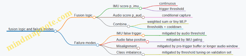
Step 5: Training and evaluation with practical checks
You train each stage with the same event definition and consistent labeling.
IMU training:
- Positive: windows that overlap the event onset by at least 50 ms.
- Negative: windows far from events.
Audio training:
- Positive: audio windows that contain the event sound burst.
- Negative: background audio segments.
Key evaluation metric: measure event-level performance, not just per-window accuracy. A single event may produce multiple overlapping windows, so you should count a detection once per event.
Example evaluation procedure:
- For each ground-truth event, check whether any fused decision occurs within a tolerance window (e.g., ±150 ms).
- Compute precision and recall at the event level.
Step 6: Resource budgeting with concrete numbers
Assume:
- IMU inference runs every 50 ms.
- Audio inference runs only when triggered.
If your IMU trigger threshold is tuned so that audio runs on average 10% of the time, total compute becomes manageable.
Practical measurement example:
- IMU inference time: 2 ms
- Audio inference time: 15 ms
- Average audio duty cycle: 10%
- Average inference load: \(2\text{ ms} + 0.1\times 15\text{ ms} = 3.5\text{ ms}\) per 50 ms cycle
This leaves time for buffering and preprocessing.
Step 7: Firmware implementation details that prevent headaches
- Use a ring buffer for audio so you can include pre-trigger audio.
- Keep tensor allocations static; avoid dynamic memory.
- Quantize preprocessing constants once and reuse them.
- Log only summary values: \(p_{imu}\), \(p_{aud}\), and fused \(S\), not raw streams.
Example debug trace (one event):
- t=1.000s: \(p_{imu}=0.41\) → trigger audio capture
- t=1.050s: audio window ready
- t=1.050s: \(p_{aud}=0.78\)
- fused \(S=0.4\times0.41+0.6\times0.78=0.64\) → below detect threshold, but above suppress threshold
- next decision at t=1.350s (cooldown logic): \(S=0.73\) → detect
This trace helps you see whether the system is failing due to gating, audio specificity, or threshold settings.
Mind map: what to tune first
Summary of the case study
Gated fusion turns multi-sensor complexity into a manageable pipeline: an always-on IMU stage provides timing and reduces unnecessary audio processing, while an audio stage adds specificity. The fusion step stays simple enough to debug and cheap enough to run in real time, and the evaluation focuses on event-level correctness rather than window-level scores.
14. Deployment Practices and Maintainable Edge ML Systems
14.1 Firmware and Model Update Workflows With Version Control
Updating a TinyML device is mostly about controlling change: you want the firmware and the model to move forward together, or not at all. The workflow below treats updates as a small, testable system with explicit versions, clear rollback rules, and measurable outcomes.
Mind map: update workflow and version control
1) Define a compatibility contract (before you ship anything)
A model update is not just “new weights.” It can change input expectations, preprocessing behavior, and output interpretation. Write down a contract that both firmware and model agree on.
Include these fields in the model metadata:
model_id: stable identifier for the task (e.g.,gesture_v1).model_version: human-readable increment (e.g.,3).model_hash: hash of the model binary.input_spec: shape and dtype (e.g.,[1, 96, 40]float32 or int8).preprocess_spec: parameters used to produce the model input (e.g., window length, overlap, scaling constants).output_spec: class count and any fixed mapping.
Then in firmware, store a firmware_model_compat table that lists which model_id values and input_spec patterns are supported. A simple rule works well: firmware refuses to activate a bundle if the contract fields don’t match.
Example:
- Firmware expects
input_spec: [1, 96, 40]int8. - Model metadata says it was exported for float32.
- The update is rejected during validation, not after activation.
This one check prevents a surprising number of “it runs but accuracy is garbage” incidents.
2) Use versioning that answers two questions
You need version numbers to answer:
- “What exactly is running?”
- “Can this firmware run that model?”
A practical approach:
- Firmware:
fw_versionas semver or a monotonic integer. - Model:
model_id+model_version+model_hash. - Bundle:
bundle_versionthat ties firmware and model together.
Example bundle manifest fields:
bundle_version:2026.03.25.1fw_min_required:1.8.0fw_max_supported:1.9.x(or a single exact version if you prefer strictness)model_id:keyword_spot_v2model_hash:...
If you keep fw_min_required and fw_max_supported, you can avoid accidental activation of a model on incompatible firmware.
3) Package updates as atomic bundles
Treat the update as one unit even if it contains multiple files. A bundle should include:
model.bin(or multiple partitions if needed)metadata.json(contract fields)config.binorconfig.json(thresholds, calibration constants)manifest.json(bundle version, hashes)
Why include config in the bundle? Because thresholds and preprocessing parameters are part of the effective model behavior. If you update weights but leave thresholds behind, you get inconsistent outputs.
Example:
- Model update improves separation between classes.
- Thresholds remain tuned for the old model.
- The device starts rejecting too many events.
- Bundling config prevents that mismatch.
4) Validate before activation (and be specific about failures)
A good validation phase checks:
- File integrity: verify
model_hashmatches the manifest. - Metadata integrity: parse and verify required fields exist.
- Contract match: compare
input_specandpreprocess_spec. - Runtime readiness: confirm required operators exist in the firmware build.
Return a structured result code so you can diagnose issues without guesswork.
Example result codes:
OKERR_HASH_MISMATCHERR_CONTRACT_INPUT_SPECERR_PREPROCESS_PARAM_MISMATCHERR_UNSUPPORTED_OPERATORERR_METADATA_PARSE
5) Activation with rollback: keep the previous bundle
Activation should be a pointer swap, not a destructive overwrite. Store:
active_bundle_slot(e.g., slot A or slot B)previous_bundle_slot(the other slot)
Flow:
- Download to inactive slot.
- Validate in inactive slot.
- Activate by updating
active_bundle_slot. - Run a short health check.
- If health check fails, revert
active_bundle_slotto the previous slot.
Health check ideas that don’t require fancy infrastructure:
- Run inference on a fixed test input captured during development.
- Confirm output tensor shape and basic numeric sanity (e.g., not all zeros, not NaNs).
- Confirm inference completes within the expected time window.
Example:
- After activation, the device runs one inference on a known sample.
- If it times out or produces invalid output, rollback triggers.
6) Minimal logging for update outcomes
You don’t need verbose logs, but you do need a few fields stored in non-volatile memory:
last_update_result_codelast_update_bundle_versionlast_update_model_hashboot_counter_since_activation
This helps you answer: “Did the update fail during validation, or after activation?”
7) Mind map: version control artifacts and responsibilities
8) Example: a simple manifest and activation logic
Below is a compact manifest structure and a validation/activation pseudocode sketch.
{
  "bundle_version": "2026.03.25.1",
  "fw_min_required": "1.8.0",
  "fw_max_supported": "1.9.9",
  "model": {
    "model_id": "keyword_spot_v2",
    "model_version": 3,
    "model_hash": "sha256:...",
    "input_spec": {"shape": [1, 96, 40], "dtype": "int8"},
    "preprocess_spec": {"window_ms": 1000, "overlap": 0.5}
  },
  "config": {"threshold": 0.72, "class_map_hash": "sha256:..."}
}
// Pseudocode: validate then activate with rollback
result = validate_bundle(bundle, fw_version, runtime_caps);
if (result != OK) return result;
write_bundle_to_inactive_slot(bundle);
set_active_slot(inactive_slot);
health = run_health_check(test_input);
if (health != OK) {
  set_active_slot(previous_slot);
  return ERR_HEALTH_CHECK_FAILED;
}
store_last_update_status(OK, bundle.version, bundle.model.hash);
return OK;
9) Practical best practices that prevent common failures
- Lock preprocessing definitions to the bundle. If preprocessing changes, treat it like a model change.
- Fail fast on contract mismatches. Reject during validation rather than activating and hoping.
- Keep two slots. One for the new bundle, one for rollback.
- Use a deterministic test input for health checks. It should be stable across builds.
- Record what ran. Store
model_hashandbundle_versionso you can correlate behavior with artifacts.
When firmware and model updates follow these rules, the device becomes predictable: updates either activate cleanly or revert cleanly, and the reason is stored as a code instead of a mystery.
14.2 Managing Configuration, Calibration, and Thresholds
Edge deployments fail in boring ways: a threshold is off by one, a calibration constant is stale, or a configuration value is interpreted in the wrong unit. This section shows how to keep those details consistent across training, conversion, firmware, and updates.
Configuration as a Contract
Treat configuration like an interface between your model and your firmware.
What to store (and why):
- Input normalization parameters (scale, offset, expected ranges): ensures the same preprocessing math is used at training and inference.
- Windowing parameters (window length, hop/stride, overlap): prevents “same model, different framing” accuracy drops.
- Model I/O contracts (tensor shapes, quantization zero-points/scales if your runtime needs them): avoids silent mismatches.
- Decision parameters (thresholds, hysteresis, minimum confidence): controls behavior under uncertainty.
- Version identifiers (model hash, preprocessing version, calibration version): makes it possible to reproduce a device’s behavior.
Easy example:
- Training used accelerometer values in m/s², but firmware reads g and multiplies by 9.81 only for some axes. Your model still runs, but the normalized values shift, and the threshold becomes meaningless.
Best practice: include a unit tag in configuration and enforce it in firmware (e.g., reject configs that claim “m/s²” while the sensor driver reports “g”).
Calibration: Separate “Sensor Reality” From “Model Math”
Calibration constants correct sensor behavior; preprocessing math prepares inputs for the model.
Common calibration types:
- Offset calibration (bias removal): e.g., subtract mean when the device is stationary.
- Scale calibration (gain correction): e.g., compensate for sensor sensitivity differences.
- Axis alignment (rotation): e.g., map sensor axes to device axes.
- Clipping/range checks: detect saturation and mark samples as invalid.
A practical IMU example:
- During manufacturing, measure bias for each axis while the device rests.
- Store
bias_x, bias_y, bias_zin non-volatile memory. - In firmware, compute
x_corr = x_raw - bias_xbefore windowing. - Then apply normalization used by the model (scale/offset to match training).
If you mix these steps—say, you bake bias removal into preprocessing during training but not in firmware—you’ll see consistent misclassification that looks like “threshold trouble,” even though the threshold is fine.
Thresholds: Make Them Deterministic and Testable
Thresholds decide what the system does. They should be explicit, measurable, and stable under small input noise.
Threshold categories:
- Single-threshold confidence:
if score >= T then class = k. - Top-k with margin: choose class only if
score_best - score_second >= M. - Hysteresis for state machines: require different thresholds for entering vs leaving a state.
- Reject option: output “unknown” when confidence is too low.
Example: hysteresis for a wake gesture
- Enter “gesture detected” when
score >= 0.75. - Exit when
score <= 0.55. This prevents rapid toggling when the score hovers around a single value.
Example: top-2 margin
- Let
s1be best score ands2second best. - Decide only if
s1 - s2 >= 0.10. This reduces false positives when multiple classes are similarly plausible.
Calibration and Threshold Workflow (End-to-End)
Use a workflow that keeps the math consistent and produces artifacts you can verify.
-
Define preprocessing math in one place
- Write down the exact normalization formula used in training.
- Mirror it in firmware with the same parameter names.
-
Calibrate sensors on the device
- Run a short routine when the device is stationary.
- Store calibration constants with a calibration version.
-
Run an on-device or offline threshold sweep
- For a labeled validation set, compute metrics across candidate thresholds.
- Pick thresholds based on the required tradeoff (false positives vs false negatives).
-
Freeze thresholds in configuration
- Store final values plus the evaluation dataset identifier (or at least a version tag).
-
Verify with a regression test
- Use a fixed set of recorded inputs.
- Confirm that firmware outputs match expected decisions.
Mind Maps
Mind map: Configuration contents and ownership
Mind map: Calibration vs preprocessing vs thresholds
Concrete Example: A Configuration Schema
Below is a compact schema you can adapt. The key idea is that each parameter has a clear unit, version, and owner.
{
  "units": {"accel": "m/s^2"},
  "preprocessing": {
    "window_ms": 100,
    "hop_ms": 20,
    "norm": {"scale": 0.015, "offset": -1.2}
  },
  "calibration": {
    "version": 3,
    "bias": {"x": 0.012, "y": -0.008, "z": 0.021}
  },
  "decision": {
    "type": "hysteresis",
    "enter": 0.75,
    "exit": 0.55,
    "min_hold_ms": 200
  },
  "model": {
    "hash": "a9f3...",
    "preprocess_version": 7
  }
}
Why this helps: if a device reports preprocess_version: 7 but firmware expects version 6, you can stop using the config and fall back to a safe mode rather than guessing.
Practical Checks in Firmware
Add small checks that catch common mistakes early.
- Range validation: if normalized inputs exceed expected bounds by a large margin, mark the sample invalid.
- Unit enforcement: if
units.acceldoesn’t match the sensor driver mode, refuse to apply normalization. - Threshold sanity: ensure
exit < enterfor hysteresis; ensure thresholds are within[0,1]for confidence scores. - Version matching: compare
model.hashandpreprocess_versionagainst what the firmware was built for.
Example sanity rule: for hysteresis, if enter <= exit, the state machine can get stuck. Detect it and log a configuration error.
Putting It Together: A Simple Decision Loop
A clean loop keeps calibration, preprocessing, and thresholding distinct.
- Read raw sensor sample.
- Apply calibration constants to get corrected values.
- Buffer samples into windows.
- Preprocess window into model input tensor.
- Run inference to get scores.
- Apply threshold logic to update state.
When these steps are separated in code, it becomes easier to change one piece without accidentally breaking another. That separation is the difference between “tuning thresholds” and “fixing the real cause.”
14.3 Building a Device Side Calibration Routine With Examples
Device-side calibration is the part of your system that turns “the model expects X” into “the device actually measures X.” It’s not about making the sensor perfect; it’s about making the input consistent enough that the model’s thresholds and quantization assumptions still make sense.
What to calibrate (and what not to)
Start by listing the inputs your model consumes and deciding which ones drift in the field.
- Calibrate scale and offset when sensors drift with temperature, mounting, or supply voltage.
- Calibrate alignment when axes are rotated or the device is mounted differently.
- Calibrate thresholds when your model outputs a score that depends on preprocessing ranges.
- Do not calibrate everything every boot. If you recalibrate a stable parameter repeatedly, you add noise and waste power.
A practical rule: calibrate parameters that affect preprocessing and input normalization, not parameters that only affect postprocessing.
A simple mind map for calibration
Calibration constants: keep them small and explicit
Store only what you need. A good calibration record is a fixed-size struct with a version number and a checksum.
Example calibration parameters for an IMU accelerometer:
acc_offset[3]in sensor unitsacc_scale[3](or a single scalar if you assume uniform scale)acc_alignmentas a 3x3 matrix or a compact representationtemp_coeffif you apply temperature compensation
Keep units consistent. If your preprocessing expects normalized values in \([-1,1]\), then your calibration should produce values that can be mapped into that range deterministically.
Boot-time quick calibration: offset from a stationary window
If your device can be stationary at boot (common for wearables and fixed installations), you can estimate offsets by averaging.
Idea: collect \(N\) samples over \(T\) seconds, assume the mean acceleration is close to gravity, and compute offsets.
For accelerometer axes: \[ \hat{b} = \frac{1}{N} \sum_{i=1}^{N} a_i \] Then subtract \(\hat{b}\) from future readings.
Easy example:
- Sampling rate: 100 Hz
- Boot window: 0.5 s → \(N=50\)
- For each axis, compute mean and store as
acc_offset.
Sanity check: ensure the magnitude of the mean is plausible. \[ |\hat{b}| \in [g-\epsilon, g+\epsilon] \] If it fails, keep previous calibration and mark the new attempt as invalid.
Temperature compensation: linear correction with guardrails
Temperature drift is common for analog front ends and MEMS sensors. A simple approach is a linear model: \[ \text{offset}(T) = b_0 + k(T-T_0) \]
Device-side routine:
- Read temperature \(T\).
- Compute corrected offset: \(b(T)=b_0+k(T-T_0)\).
- Apply \(a_{corr}=a_{raw}-b(T)\).
Example with guardrails:
- Store
b0andkfrom a factory or first-run calibration. - Clamp \(b(T)\) to a maximum change allowed per degree to prevent runaway constants if temperature sensing is noisy.
Axis alignment: calibrate rotation using gravity
If your model expects a specific axis convention, you need to map device axes to model axes.
Assumption: during calibration, the device is placed in a known orientation (e.g., screen up). Gravity provides a reference.
Example workflow (accelerometer-only):
- Ask the user to place the device flat (or detect a “stationary and stable” condition).
- Compute the gravity direction vector \(\hat{g}_d\) in device coordinates from averaged samples.
- Compute the rotation that maps \(\hat{g}_d\) to the model’s expected gravity direction \(\hat{g}_m\).
If you only care about aligning “up,” you can build a rotation that aligns one vector and leaves rotation around that axis unspecified. For many classification tasks, that’s enough.
Sanity check: verify that the aligned gravity direction matches within an angular tolerance. \[ \theta = \arccos(\hat{g}_d \cdot \hat{g}_m) \] Reject alignment if \(\theta\) is too large.
Threshold calibration: calibrate the decision boundary, not the model
Sometimes your model outputs a score \(s\) and you choose a threshold \(\tau\) to decide “event vs no event.” If preprocessing normalization changes slightly, the score distribution shifts.
A device-side threshold calibration can be done using a short “no-event” window.
Example: keyword spotting or button tap detection.
- At boot, record \(M\) seconds of audio while the device is assumed idle.
- Compute the mean and spread of the score: \(\mu\) and \(\sigma\).
- Set threshold \(\tau = \mu + c\sigma\), where \(c\) is chosen to match your desired false positive rate.
Guardrail: cap \(\tau\) to a reasonable range derived from training-time thresholds so the device can’t drift into a bad regime due to unusual ambient conditions.
Calibration routine structure: a repeatable state machine
Implement calibration as a small state machine so it’s testable and doesn’t block inference forever.
- State: LoadCalibration
- Read constants from NVM
- Validate checksum and version
- State: DecideRun
- If constants valid and not expired → skip
- Else if device is stationary/idle → run quick calibration
- State: CollectSamples
- Gather N samples for each required sensor
- Track mean and variance online
- State: EstimateConstants
- Compute offsets/scales/thresholds
- Apply temperature correction if available
- State: Validate
- Sanity checks (ranges, magnitudes, angles)
- If fail → keep previous constants
- State: Save
- Write new constants with checksum
- Update “last calibrated” timestamp
Concrete example: IMU gesture classifier calibration
Goal: keep normalized acceleration features consistent.
Routine:
- Stationary detection: require low variance in accelerometer magnitude over 0.5 s.
- Offset estimation: compute
acc_offset[3]from the stationary window. - Temperature correction: apply \(b(T)=b_0+k(T-T_0)\) if coefficients exist.
- Gravity alignment: compute gravity direction and align “up” to the model’s expected axis.
- Store constants and record a small summary:
offset_norm,alignment_angle.
Why this works: gesture models often rely on relative motion patterns. Offsets and axis conventions distort those patterns, especially after quantization.
Concrete example: audio keyword spotting threshold calibration
Goal: stabilize the score threshold under changing noise.
Routine:
- Idle window: at boot, record 2 seconds of audio.
- Compute score distribution: run inference on each frame and collect scores.
- Set threshold: \(\tau = \mu + 2\sigma\) (with clamping).
- Save threshold with a timestamp.
- During operation: if the device detects long idle periods, occasionally refresh \(\tau\) using a low duty cycle.
Why this works: it adjusts the decision boundary to the current background without changing the model weights.
Verification: measure calibration quality without drowning in logs
Use lightweight checks:
- Constant validity: checksum, version, and range checks.
- Feature sanity: after preprocessing, verify that normalized inputs fall into expected bounds (e.g., mean near 0, typical magnitude near 1).
- Decision sanity: during calibration windows, ensure the system doesn’t produce extreme scores.
A good calibration routine fails gracefully: if it can’t trust the sensor state, it keeps the previous constants and continues inference.
Implementation notes that prevent common headaches
- Use fixed-point where your preprocessing does. If your firmware uses \(q\)-format math, calibrate in the same numeric domain.
- Avoid recalibrating while moving. Stationary assumptions are the foundation of offset estimation.
- Keep calibration time bounded. A calibration that takes too long can break real-time behavior.
- Store only what you can validate. If you can’t sanity-check a constant, don’t store it.
With these pieces in place, device-side calibration becomes a controlled, testable step that makes your edge model behave like it did during development—without requiring a lab every time you ship a device.
14.4 Secure Packaging and Integrity Checks for Artifacts
Edge ML deployments usually fail in boring ways: a file got truncated, a model was converted with different settings, or firmware and model versions no longer agree. Secure packaging and integrity checks aim to make those failures obvious and early, with clear error messages and predictable behavior.
What you are protecting (and what you are not)
You typically package these artifacts:
- Model file (converted format used by your runtime)
- Metadata (input shape, quantization parameters, label mapping, preprocessing version)
- Firmware image (or a manifest that firmware can verify)
- Optional calibration data (scales/offsets used by preprocessing)
You are not trying to hide the model from inspection. You are trying to ensure the device runs the intended model with the intended preprocessing and firmware.
A practical packaging layout
Use a single “bundle” file (or a directory that is zipped into one file) with a manifest and checksums.
Bundle contents
model.bin(ormodel.tflite/ runtime-specific binary)metadata.jsonmanifest.jsonsignatures/(optional, if you use signing)
Manifest fields to include
bundle_version(for your own format evolution)model_hash(hash ofmodel.bin)metadata_hash(hash ofmetadata.json)firmware_compat(minimum/maximum firmware build IDs)preprocess_compat(a version string or hash of preprocessing code/config)created_at(optional, but useful for logs)
A good manifest is small and deterministic. Determinism matters because you want the hash to match across machines.
Mind map: packaging and integrity checks
Integrity checks: the minimum set that pays off
Start with checks that are easy to implement and cheap to run.
-
Size checks
- Store
model_size_bytesandmetadata_size_bytesinmanifest.json. - Reject bundles where sizes differ before hashing.
- This catches truncated downloads quickly.
- Store
-
Hash checks
- Compute
SHA-256(model.bin)andSHA-256(metadata.json). - Store those digests in
manifest.json. - On device, recompute and compare.
- Compute
-
Manifest integrity
- Hash the manifest itself, or sign it.
- If you only hash model and metadata, an attacker could swap the manifest to point to different hashes. Signing prevents that.
-
Metadata contract validation
- Validate that
metadata.jsonmatches what firmware expects. - Examples:
input_shapeequals the runtime’s configured input tensor shapequantizationfields match the expected scheme (e.g., per-tensor int8)label_countmatches the firmware’s label handling
- Validate that
Authenticity: signing the manifest (optional but recommended)
If you can afford it, sign the manifest so the device can verify that the bundle came from your build pipeline.
Signing approach
- Sign
manifest.json(not the model) because the manifest is small. - Store the public key in firmware.
- Device verifies signature before any heavy work.
Why sign the manifest?
- It binds together: model hash, metadata hash, compatibility rules, and version strings.
- You avoid signing large binaries and keep verification fast.
Example manifest (illustrative)
{
  "bundle_version": 1,
  "model": {
    "filename": "model.bin",
    "sha256": "...",
    "size_bytes": 123456
  },
  "metadata": {
    "filename": "metadata.json",
    "sha256": "...",
    "size_bytes": 7890
  },
  "firmware_compat": {
    "min_build_id": 1200,
    "max_build_id": 1299
  },
  "preprocess_compat": {
    "preprocess_version": "imu_v3_norm_v2"
  }
}
Device-side verification flow (concrete)
A robust flow is: verify cheap things first, then expensive things, then load.
-
Parse bundle
- Ensure required files exist.
- Reject unknown extra files if you want strictness.
-
Check sizes
- Compare actual file sizes to manifest values.
-
Verify hashes
- Compute SHA-256 for
model.binandmetadata.json. - Compare to manifest.
- Compute SHA-256 for
-
Verify signature (if present)
- Verify signature over
manifest.json. - If signature is missing but your policy requires it, reject.
- Verify signature over
-
Validate metadata contracts
- Confirm
input_shapeanddtype. - Confirm normalization parameters version.
- Confirm label mapping size.
- Confirm
-
Atomic install
- Write bundle to a staging area.
- Only swap the “active” model pointer after all checks pass.
-
Log a structured result
- Record: bundle version, model hash prefix, and failure reason.
- Keep logs short; store full hashes only if you have space.
Example error codes and messages
Clear errors reduce time spent guessing.
E_BUNDLE_MISSING_FILEE_BUNDLE_SIZE_MISMATCHE_BUNDLE_HASH_MISMATCHE_MANIFEST_SIGNATURE_INVALIDE_METADATA_CONTRACT_MISMATCHE_FIRMWARE_INCOMPATIBLE
Example message (device log):
E_METADATA_CONTRACT_MISMATCH: expected input_shape=[1,96,3], got=[1,64,3]
Mind map: metadata contract validation
Example: contract validation rules for IMU
Suppose your firmware expects a 3-axis IMU window with 96 samples.
-
Firmware expects:
input_shape = [1, 96, 3]preprocess_version = "imu_v3_norm_v2"label_count = 6
-
Device checks:
- If
metadata.input_shapediffers, reject withE_METADATA_CONTRACT_MISMATCH. - If
preprocess_versiondiffers, reject even if shapes match; preprocessing drift can silently degrade accuracy.
- If
Atomic install example (staging then swap)
staging/ (new bundle)
  - model.bin
  - metadata.json
  - manifest.json
active/ (currently running)
  - model.bin
  - metadata.json

Flow:
1) Verify staging bundle.
2) If OK: rename staging -> active (or update pointers).
3) If fail: delete staging, keep active unchanged.
Putting it together: a cohesive policy
A simple policy that works well:
- Always enforce size + hash checks.
- Always enforce metadata contract validation.
- Use manifest signing when you control the build pipeline and can store a public key.
- Install bundles atomically so a failed update never leaves the device without a working model.
When these checks are in place, failures become deterministic: either the bundle is correct, or the device refuses it with a specific reason. That’s the whole point—less guessing, more certainty.
14.5 Documentation Templates for Reproducible Deployments
Reproducible deployments start with boring, consistent records. When something changes—data, model, compiler flags, thresholds, or firmware—you want to answer two questions quickly: “What exactly is running?” and “How did we get it?” The templates below are designed to be filled in once and reused for every release.
Release Record (the “what is running” page)
Use this as the top-level document for each deployed version.
Template: ReleaseRecord.md
- Release ID: (e.g., FW-1.3.0 / MODEL-2026-03-24 / CFG-2)
- Device family: (MCU/SoC, board revision)
- Firmware version: (git commit hash)
- Model version: (training run ID, export hash)
- Runtime version: (TinyML runtime + commit hash)
- Preprocessing version: (code commit hash for scaling/windowing)
- Input contract:
- Sample rate:
- Window length:
- Feature shape:
- Normalization constants:
- Output contract:
- Output tensor names/shapes
- Class labels mapping
- Decision logic:
- Threshold(s)
- Smoothing/majority vote settings (if any)
- Reject behavior (what happens when confidence is low)
- Quantization details:
- Quantization scheme (e.g., int8 symmetric/asymmetric)
- Calibration dataset ID and size
- Build artifacts:
- Model file name + checksum
- Firmware binary name + checksum
- Verification summary:
- On-device test suite name
- Pass/fail criteria
- Measured latency and peak memory
- Known limitations:
- Edge cases and expected failure modes
Example (filled-in excerpt):
- Release ID:
FW-1.3.0 / MODEL-IMU-GEST-041 / CFG-7 - Input contract: Sample rate 100 Hz, window length 1.0 s, overlap 50%, feature shape
[1, 6, 100] - Decision logic: threshold 0.72, 3-frame majority vote, reject outputs
UNKNOWN - Quantization: int8 asymmetric activations, per-channel weights
- Verification: 5000 on-device samples, accuracy ≥ 92%, max latency ≤ 12 ms
Model Card for Embedded Inference (the “how it behaves” page)
This document focuses on behavior under constraints: quantization, preprocessing, and decision thresholds.
Template: ModelCardEmbedded.md
- Purpose: task and expected operating conditions
- Training data summary:
- Sensor types and mounting constraints
- Class list and label definition
- Dataset IDs used for train/val/test
- Preprocessing pipeline:
- Windowing parameters
- Scaling method and constants
- Any filtering (e.g., moving average)
- Architecture summary:
- Model type and layer count
- Input/output shapes
- Quantization and calibration:
- Calibration dataset ID
- Representative sample count
- Notes on out-of-range handling
- Evaluation results:
- Float model metrics (if available)
- Quantized model metrics
- Confusion highlights (which classes fail and why)
- Thresholding guidance:
- Recommended threshold and rationale
- Tradeoff: false accepts vs false rejects
- Failure modes:
- Sensor saturation behavior
- Motion blur / low SNR behavior
- Unseen classes behavior
- Reproducibility checklist:
- Exact training script version
- Exact export settings
- Exact preprocessing code version
Example (thresholding section):
- Recommended threshold: 0.72
- Rationale: At 0.72, false rejects drop below 3% for “tap” while false accepts remain under 1% for “no tap” during the validation set.
Preprocessing Contract (the “same numbers in, same numbers out” page)
Most deployment mismatches come from preprocessing drift. Treat preprocessing like an API.
Template: PreprocessContract.md
- Input units: (e.g., m/s², degrees/s)
- Raw-to-physical conversion:
- ADC scaling formula
- Calibration offsets
- Normalization:
- Mean/variance or min/max values
- Where constants are stored (firmware vs model)
- Windowing:
- Window length
- Overlap
- Alignment rule (start index)
- Feature extraction:
- Feature type (raw samples, spectrogram bins, statistical features)
- Output tensor shape
- Quantization of inputs:
- Input scaling factor
- Clipping behavior
- Determinism notes:
- Integer math rules
- Rounding mode
Example (determinism note):
- Use integer rounding toward zero for fixed-point scaling to match the training-time simulation.
Artifact Manifest (the “checksum everything” page)
This is a short file that makes it hard to accidentally mix versions.
Template: ArtifactManifest.txt
- Firmware binary:
app.binSHA256:... - Model file:
model.tfliteSHA256:... - Labels file:
labels.jsonSHA256:... - Config file:
runtime_config.jsonSHA256:... - Preprocessing constants:
norm_constants.binSHA256:... - Build metadata: compiler version, flags
Verification Plan Template (the “prove it works the same way” page)
A verification plan should specify what is measured and what counts as a pass.
Template: VerificationPlan.md
- Test scope:
- Preprocessing correctness
- Inference correctness
- Decision logic correctness
- Performance constraints
- Test datasets:
- Dataset IDs
- Sample counts
- Coverage notes (e.g., different users, different noise levels)
- Reference outputs:
- Expected float outputs (optional)
- Expected quantized outputs (preferred)
- Metrics:
- Accuracy / F1
- Latency (p50/p95)
- Peak RAM / arena usage
- Power measurement method (if used)
- Pass criteria:
- Accuracy ≥ X%
- Latency ≤ Y ms
- Arena ≤ Z bytes
- Logging requirements:
- What to record per test run
- How to store logs without truncation
Mind maps
Mind map: Reproducible deployment documentation flow
Mind map: Common mismatch sources and where to document them
Practical example: one release, five files
Imagine a gesture classifier update.
- ReleaseRecord.md states: firmware commit
a1b2c3, modelIMU-GEST-041, threshold0.72, and decision uses 3-frame majority vote. - ModelCardEmbedded.md lists calibration dataset
CAL-IMU-1200and reports quantized accuracy 93.1% with the same preprocessing. - PreprocessContract.md defines the fixed-point rounding rule and the exact window overlap.
- ArtifactManifest.txt includes checksums for
model.tflite,labels.json, andnorm_constants.bin. - VerificationPlan.md specifies that on-device tests run 5000 samples and must meet latency ≤ 12 ms and accuracy ≥ 92%.
When a field issue appears, you can compare the Release ID and checksums first, then inspect the preprocessing contract and threshold logic second. That order saves time because it separates “did we change something?” from “did the change behave differently?”
15. Practical Troubleshooting Guide for TinyML Projects
15.1 Diagnosing Accuracy Drops After Quantization
Quantization usually changes two things at once: how numbers are represented (scale/zero-point) and how rounding behaves inside each operator. When accuracy drops, the goal is to find which change caused the damage, then confirm it with a small, measurable experiment.
First: confirm the drop is real (and not a pipeline mismatch)
Before blaming quantization, verify that the quantized model is fed the same way as the float model.
- Input preprocessing parity: Ensure the same resize/crop, normalization, and channel order are used for both runs. A common failure is “float path uses mean/std, quant path uses min/max scaling.”
- Tensor shape and layout: Confirm the input tensor shape matches the exported contract. If the model expects
[1, H, W, C]but you feed[1, C, H, W], quantization will not be the only problem—but it will be the first one you notice. - Threshold parity: If you use a confidence threshold or argmax post-processing, keep it identical across float and quantized tests.
Quick check example: Run 100 samples through float inference and record top-1 accuracy. Then run the same 100 samples through the quantized model using the exact same preprocessing code path. If accuracy is identical, the issue is likely not quantization itself.
Mind map: where accuracy can go wrong
Step 1: compare intermediate activations (the fastest way to localize)
If you can instrument the runtime to dump tensors, compare float vs quantized activations at a few strategic points.
What to look for:
- Range mismatch: Quantized activations may be heavily clipped (many values stuck at min/max).
- Scale mismatch: Values may be compressed into a narrow band, reducing separability.
- Distribution shift: The mean/variance changes significantly layer-to-layer.
Practical example (layer localization):
- Pick three layers: the first conv, a mid-layer, and the final logits.
- For a fixed input batch, compute float activations.
- Quantize activations using the same scales/zero-points used by the model (or dump quantized tensors if supported).
- Plot histograms or compute simple stats: min, max, mean, and percent of values at extremes.
If the first conv output is already clipped, the calibration ranges are likely wrong. If early layers look fine but logits collapse toward a single class, the problem is often in later layers or the final activation/softmax handling.
Step 2: audit calibration (range selection is the usual culprit)
Most post-training quantization depends on calibration data to estimate activation ranges. Accuracy drops often trace back to calibration that doesn’t represent real inputs.
Common calibration mistakes (with easy examples):
- Calibration set too small: If you calibrate with 50 samples but your sensor has multiple operating modes, ranges may miss rare but important patterns.
- Calibration set not representative: For keyword spotting, calibrating only with clean audio might fail on noisy recordings because activation ranges become too tight.
- Outliers dominate: If a few extreme samples appear in calibration, the range expands, and most normal values get fewer effective quantization levels.
Concrete diagnostic:
- Run calibration with two different subsets: one “typical” and one “mixed.”
- Compare accuracy for each quantized model.
- If the “mixed” calibration improves accuracy, your original calibration likely under-covered important variability.
Step 3: check per-channel vs per-tensor quantization
Per-channel quantization (often for weights) can preserve accuracy better because each output channel gets its own scale. If you accidentally force per-tensor quantization, some layers may lose too much precision.
Example reasoning:
- Suppose a depthwise conv has channels with very different magnitudes.
- With per-tensor quantization, one global scale must cover all channels.
- Small-magnitude channels then quantize with too few distinct values, making their features less distinguishable.
Diagnostic approach:
- Quantize the same float model twice: once with per-channel enabled (where supported) and once with per-tensor.
- Compare accuracy and, if possible, activation histograms for the affected layers.
Step 4: look for saturation and clipping patterns
Quantized activations are limited by integer ranges and chosen scales. Saturation is a strong sign that the model’s dynamic range doesn’t fit the quantization scheme.
How to detect saturation without fancy tools:
- For a dumped quantized activation tensor, compute the fraction of values equal to the minimum representable integer and the fraction equal to the maximum.
- High fractions suggest clipping.
Example:
- If a ReLU output has 30% of values at the max integer, the layer likely saturates.
- That saturation can flatten differences between classes, especially if the saturated layer is near the classifier head.
Step 5: verify conversion and operator support
Sometimes accuracy drops because the conversion process changes the computation graph.
What to check:
- Are there warnings about unsupported operators or fallback paths?
- Did the converter fuse layers in a way that changes expected behavior (e.g., batch normalization folding)?
- Are there differences in how softmax or logit scaling is handled?
Example: If your float model applies softmax in Python but the quantized model outputs logits, comparing “probabilities” to “logits” will look like an accuracy drop even when the underlying classification is fine. Keep the comparison at the same stage: either both at logits (argmax) or both at probabilities.
Step 6: isolate runtime issues (the boring but real category)
Quantization errors are not always quantization. Runtime mismatches can corrupt results.
Checklist:
- Confirm the runtime uses the correct quantized dtype (e.g., int8 vs uint8) for each tensor.
- Ensure the input zero-point and scale are applied correctly.
- If you use an arena allocator, confirm tensor buffers don’t overlap.
Example: A single incorrect buffer size can cause only some layers to be wrong, which can look like “quantization made it worse” because the quantized model is more memory-tight.
Step 7: use a minimal “ablation” strategy
When you can’t easily dump intermediates, you can still localize by changing one thing at a time.
Ablation ideas:
- Compare float vs quantized with the same preprocessing and post-processing.
- Quantize only weights (if your tool supports it) while keeping activations in float.
- Quantize only activations while keeping weights float.
Interpretation:
- If weight-only quantization preserves accuracy, the issue is likely activation calibration or activation quantization.
- If activation-only quantization drops accuracy, focus on activation ranges and clipping.
Summary: a practical diagnostic path
- Confirm preprocessing and post-processing parity.
- Compare intermediate activations at a few layers to localize.
- Re-check calibration representativeness and outliers.
- Verify per-channel settings for weights.
- Look for saturation/clipping using extreme-value fractions.
- Check conversion warnings and output stage consistency.
- Validate runtime dtype handling and memory safety.
Accuracy drops after quantization are usually explainable with measurements rather than guesses. Once you can point to the first layer where distributions diverge, the fix becomes much more specific than “try another quantization setting.”
15.2 Fixing Conversion Errors and Unsupported Operators
Conversion failures usually fall into two buckets: (1) the converter can’t map an operation to what the runtime supports, or (2) the operation maps, but the shapes, dtypes, or parameters don’t match the runtime’s expectations. The fastest way to fix either bucket is to read the error like a checklist: which node, what operator, what input/output shapes, and what constraint got violated.
A practical mind map for conversion errors
Step 1: Identify the failing node precisely
Most converters print a node name or an operator type near the error. Treat that as the starting point, not the whole story. For example, you might see something like “Unsupported operator: ResizeBilinear” or “Operator Add not supported for int8.” In both cases, the node name tells you where to look in the model graph.
Example: unsupported resize
- Your model uses
torch.nn.functional.interpolate(..., mode='bilinear'). - Conversion fails with an unsupported operator error.
- The fix is often to replace resize with a supported alternative (e.g., fixed-size input, or a different interpolation mode that maps to a supported op).
Example: unsupported add for quantized tensors
- Your model adds two branches after quantization.
- Conversion fails because the runtime only supports
Addfor certain dtypes or requires matching quantization scales. - The fix is to ensure both branches are quantized consistently before the add, or to restructure the graph so the add happens in a supported dtype region.
Step 2: Inspect tensor contracts (rank, shape, dtype)
Unsupported operators are sometimes red herrings caused by mismatched tensor contracts. A runtime might support an operator in principle, but only for specific input ranks or static shapes.
Check these four things for the failing node:
- Input rank: Convolution-like ops often expect 4D tensors:
[N, H, W, C]or[N, C, H, W]depending on the toolchain. - Static dimensions: Many embedded runtimes require fixed sizes for certain ops.
- Dtype: Quantized runtimes typically support int8/uint8 for activations and weights, with limited float support.
- Parameter constraints: Padding modes, stride values, and groups must match what the runtime implements.
Example: rank mismatch caused by a reshape
- You flatten a feature map and then apply an op that expects a 4D tensor.
- The converter might report the later op as unsupported, even though the real issue is the earlier reshape.
- Fix by moving the flatten later, or by using a supported sequence:
Conv -> Pool -> Flatten -> Dense.
Step 3: Replace unsupported operators with supported equivalents
When an operator is truly unsupported, you have three common replacement patterns.
Pattern A: Remove the need for the op via input sizing
If the unsupported op is used only to make tensors the right size (like resizing), prefer making the input size fixed upstream.
Example: fixed input instead of resize
- Instead of resizing inside the model, resize/crop in preprocessing.
- Then the model sees a fixed shape, and the converter no longer needs the resize op.
This is especially effective for image pipelines where the runtime expects a fixed input tensor.
Pattern B: Use a mathematically equivalent op the runtime supports
Some ops can be rewritten.
Example: “same padding” vs explicit padding
- If the runtime doesn’t support a padding mode variant, replace it with explicit padding using a supported padding op or by adjusting convolution parameters.
- The goal is to end up with the exact same output shape and values (within quantization tolerance).
Pattern C: Fuse or restructure the graph
Some unsupported ops appear because of graph rewrites.
Example: activation + convolution ordering
- If the model has
Conv -> BatchNorm -> ReLU, conversion might fail if BatchNorm isn’t supported. - In many toolchains, BatchNorm can be folded into Conv weights during export or by running a “fold batchnorm” step.
- If folding isn’t automatic, do it explicitly before export.
Step 4: Handle quantization-related conversion failures
Quantization errors often show up as unsupported operator variants or dtype mismatches.
Common quantization pitfalls
- Mismatched scales/zero points for elementwise ops like
AddandMul. - Per-channel vs per-tensor quantization differences for weights.
- Activation quantization not applied where the runtime expects it.
Example: int8 Add with different quantization parameters
- Two branches are quantized independently.
- Their scales differ, and the runtime’s
Addimplementation requires compatible quantization. - Fix by ensuring both branches share the same quantization scheme before the add, or by inserting a quantization step that aligns them.
A simple sanity check is to temporarily run conversion in a mode that keeps more tensors in float (if supported by your toolchain). If the float conversion succeeds but int8 fails, the issue is likely quantization contracts rather than the operator itself.
Step 5: Minimal-change debugging workflow
Avoid editing the model in large chunks. Use a “one change, one test” approach.
- Start with the smallest failing model: remove optional heads or auxiliary outputs.
- Freeze preprocessing: ensure the exported model input shape matches what you feed during conversion.
- Re-run conversion after each change.
- Compare node-by-node outputs when the toolchain provides intermediate dumps.
Example: isolate a failing branch
- If conversion fails in a multi-branch network, temporarily replace one branch with a constant tensor of the correct shape.
- If conversion succeeds, the failing branch contains the unsupported op or quantization mismatch.
Step 6: Concrete “fix recipes” for frequent unsupported ops
Below are common conversion failures and typical fixes.
| Unsupported operator symptom | Likely cause | Fix recipe |
|---|---|---|
ResizeBilinear unsupported | Resize mode/op not implemented | Resize in preprocessing; use fixed input size; or switch to a supported resize variant |
BatchNorm unsupported | Runtime lacks BN or folding not applied | Fold BN into Conv before export; ensure inference graph uses Conv with updated weights |
LayerNorm unsupported | Normalization op not implemented | Replace with a supported normalization approach (often remove LN or rewrite using supported ops) |
Add/Mul unsupported for int8 | Quantization mismatch | Align quantization parameters; ensure both inputs to elementwise ops use compatible scales/zero points |
Reshape/Transpose causes later op failure | Rank/contiguity/shape mismatch | Adjust reshape/transpose so the downstream op receives the expected rank and layout |
Step 7: Verify after conversion, not just at conversion time
A successful conversion doesn’t guarantee correct behavior. Run a small on-device test with a few representative inputs.
Example: two-input smoke test for elementwise ops
- Pick two samples that exercise both branches.
- Confirm outputs are finite and within expected ranges.
- If outputs look saturated, revisit quantization alignment for the elementwise node.
Example: shape sanity test
- Feed an input with known simple patterns (e.g., zeros, a single impulse, or a ramp).
- Check whether the output changes in the expected direction.
When you treat conversion errors as graph contract problems—operator support, tensor shape/rank, and quantization compatibility—the fixes become mechanical rather than mysterious. The goal is to make the failing node’s inputs match what the runtime can execute, then confirm with a tiny on-device test vector.
15.3 Resolving Memory Crashes and Arena Sizing Issues
Memory crashes in TinyML projects usually come from one of two places: the runtime’s memory arena is too small, or the firmware’s buffers don’t match the model’s real tensor sizes. The tricky part is that both problems can look identical at runtime: a hard fault, a watchdog reset, or silent corruption that shows up later.
What “arena” means in practice
In most embedded inference runtimes, an “arena” is a preallocated block of RAM used for intermediate tensors and scratch buffers. The model weights are stored separately (often in flash), but activations and temporary buffers live in the arena.
A common symptom pattern:
- Works in a small test, then crashes when you enable streaming or increase input length.
- Crashes only after a few inferences, suggesting a buffer overwrite rather than a one-time allocation failure.
- Crashes only in release builds, which can change memory layout and alignment.
Mind map: memory crash causes and fixes
Step 1: Confirm the crash is actually arena-related
Before changing sizes, verify what fails.
Quick checks
- Check the fault address (if your platform reports it). If it points into the arena region, you’re likely overwriting beyond the allocated block.
- Add a canary around the arena. Fill a few bytes before and after the arena with a known pattern, then check after inference.
- Run a single inference with a fixed input and no streaming. If it crashes immediately, it’s often arena sizing or tensor mismatch. If it crashes after several iterations, it’s more likely buffer reuse or concurrency.
Example: canary guard
#define CANARY 0xA5
#define ARENA_BYTES  (64 * 1024)
static uint8_t arena[ARENA_BYTES];
static uint8_t arena_pre[16];
static uint8_t arena_post[16];

void init_canary(void){
  memset(arena_pre, CANARY, sizeof(arena_pre));
  memset(arena_post, CANARY, sizeof(arena_post));
}

int canary_ok(void){
  return memcmp(arena_pre, (uint8_t[16]){CANARY}, 16)==0 &&
         memcmp(arena_post,(uint8_t[16]){CANARY}, 16)==0;
}
If canary_ok() fails after inference, you’ve confirmed an overwrite. If it stays intact but you still crash, the issue may be elsewhere (stack, ISR interference, or a pointer bug).
Step 2: Size the arena from measured peak usage
Many runtimes provide a way to estimate or report required arena size. If you don’t have that report, you can still measure by binary searching arena size.
Binary search method
- Start with a conservative arena size that you know is too small.
- Increase in steps (or binary search) until the model runs reliably for many iterations.
- Keep the smallest size that passes, then add a safety margin for future changes.
Example: binary search loop (conceptual)
- Try 32 KB → crash
- Try 48 KB → crash after a few iterations
- Try 56 KB → stable for 10,000 inferences
- Choose 56 KB + margin (e.g., 10%)
Why this works: arena usage depends on tensor lifetimes and operator implementations, which can change with input shape, preprocessing window size, and even compilation flags.
Step 3: Validate tensor shapes and preprocessing output
Arena sizing can look “wrong” when the input tensor you feed doesn’t match what the model expects.
Common mismatch cases:
- You preprocess into a buffer of the right length, but you pass a pointer with the wrong offset.
- You assume a fixed window size, but your streaming code sometimes produces a shorter window.
- You reshape or reorder channels incorrectly (e.g., HWC vs CHW).
Practical runtime verification At startup, print or log:
- Input tensor dimensions
- Output tensor dimensions
- Data type (int8, int16, etc.)
Then compare those against your preprocessing buffer size.
Example: streaming window bug Suppose your model expects 96 samples per inference.
- Your ring buffer holds 128 samples.
- Your code sometimes copies only 80 samples when the stream just started.
- The runtime still runs, but intermediate tensors become inconsistent with the expected input layout, leading to memory corruption.
Fix by gating inference until the buffer has accumulated the full window, and always copy exactly the expected number of samples.
Step 4: Check arena placement, alignment, and memory region
Even with the correct size, the arena can fail if it’s placed in a memory region with different access rules.
Things to verify
- Alignment: Many runtimes assume 4-byte alignment for int8/int16 buffers. Misalignment can cause faults on some MCUs.
- Memory region: Some MCUs have separate SRAM banks. If you place the arena in a region that’s too small or not accessible by DMA/CPU as expected, you can get crashes.
- Linker script: Ensure the arena symbol lands where you think it does.
Example: enforce alignment
#include <stdint.h>

#define ARENA_BYTES (64 * 1024)

__attribute__((aligned(16)))
static uint8_t arena[ARENA_BYTES];
If your runtime uses vectorized kernels, 16-byte alignment can matter.
Step 5: Avoid stack-related crashes
A surprisingly common failure mode is not the arena at all, but the stack.
If you call inference from a deep call chain, or you allocate large temporary arrays on the stack, you can hit stack overflow. The crash may appear during inference because that’s when the stack usage peaks.
Example: move large temporaries to static buffers
- Replace
uint8_t tmp[4096];inside a function with a static/global buffer. - Reduce local arrays used for preprocessing.
Also check ISR behavior: if an interrupt triggers while inference is running and uses the same buffers, you can corrupt memory.
Step 6: Isolate operator-specific memory spikes
Some operators allocate more scratch space than others. If you can’t get a peak arena report, isolate by simplifying.
Isolation strategy
- Temporarily replace the model with a smaller one (fewer layers) and see if the crash disappears.
- If you can’t change the model, try reducing input resolution or window length.
Example: window length effect For sequence models, increasing the number of time steps can increase intermediate activations. If you double the window, you may more than double arena usage depending on how the runtime schedules tensor lifetimes.
Step 7: Make arena sizing robust in firmware
Once you find a stable arena size, make it hard to break.
Best practices
- Define arena size as a single constant used consistently across firmware and build scripts.
- Add an assertion that the arena size is at least the runtime’s required minimum (if the runtime exposes it).
- Keep preprocessing output sizes strictly tied to model input dimensions.
Example: compile-time checks
#define MODEL_INPUT_SAMPLES 96
#define PREPROC_OUTPUT_SAMPLES 96

_Static_assert(PREPROC_OUTPUT_SAMPLES == MODEL_INPUT_SAMPLES,
               "Preprocessing output size must match model input");
This catches the “works on my bench” mismatch where someone changes preprocessing but forgets the model.
Checklist for the next crash
- Add canary guards around the arena.
- Verify input/output tensor dimensions at runtime.
- Ensure arena alignment and correct memory placement.
- Confirm stack headroom and avoid large stack temporaries.
- Gate inference until the full input window is available.
- Increase arena size using a measured approach, not guesses.
When these steps are followed in order, you usually end up with a clear answer: either the arena is genuinely too small, or the firmware is feeding the runtime something slightly different than what the model expects. In both cases, the fix is straightforward once you’ve identified which mismatch you actually have.
15.4 Debugging Timing Problems and Buffer Overruns
Timing bugs and buffer overruns usually share a theme: something “almost” fits. The system runs for a while, then a rare input pattern, a slightly slower sensor read, or a different batch size pushes execution over the edge. This section gives a practical method to find the exact moment things stop matching the design.
First: classify the failure
Before changing code, identify which symptom you have.
- Timing overrun: inference finishes late, but memory stays intact. You may see missed deadlines, growing latency, or watchdog resets.
- Buffer overrun: memory corruption appears. Symptoms include random wrong predictions, crashes, or sudden changes after a specific input length.
- Both: timing overrun triggers buffer overrun (common when a “catch-up” loop writes more samples than the buffer can hold).
A quick checklist:
- Does the failure correlate with input size (e.g., longer audio windows) or sensor rate?
- Does it correlate with first run after boot (often initialization or arena sizing) or after N iterations (often a ring buffer index bug)?
- Does it correlate with debug logging (logging changes timing and can hide or reveal races)?
Mind map: timing + buffers
Step 1: measure the loop with timestamps
You want three numbers per iteration: start time, end time, and how much data was processed. If you only measure total loop time, you’ll miss whether inference or preprocessing is the culprit.
A simple pattern is to time each stage and store the maximum observed values.
// Keep this instrumentation minimal in production builds.
uint32_t t0 = now_us();
preprocess();
uint32_t t1 = now_us();
run_inference();
uint32_t t2 = now_us();

uint32_t prep_us = t1 - t0;
uint32_t infer_us = t2 - t1;

if (prep_us > max_prep_us) max_prep_us = prep_us;
if (infer_us > max_infer_us) max_infer_us = infer_us;
Reasoning: if infer_us occasionally spikes, you likely hit cache misses, DMA contention, or a rare path (e.g., a different input branch). If prep_us spikes, look at filtering, normalization, or dynamic windowing.
Step 2: compute a real latency budget
A “budget” is not a guess; it’s a calculation from your sampling and scheduling.
If you sample at frequency (f_s) and you run inference every (N) samples, then the time between inference triggers is: \[ T_{period} = \frac{N}{f_s} \]
Your inference must fit, including overhead: \[ T_{period} \ge T_{acquire} + T_{preprocess} + T_{infer} + T_{post} \]
Example: You sample IMU at 200 Hz (
\(f_s=200\) ) and use a 100-sample window with 50-sample overlap. If you run inference every 50 new samples, then:
\[
T_{period} = \frac{50}{200} = 0.25\text{ s}
\]
If your measured worst-case infer_us is 180 ms, you’re already close. Any extra blocking call will break deadlines.
Step 3: instrument buffer fill and indices
Buffer overruns often come from index math that is correct “on average” but wrong at wrap boundaries.
Track:
- ring buffer
write_idxandread_idx count(if you use it)- maximum fill level observed
// Example ring buffer debug counters.
if (write_idx == 0 && prev_write_idx != 0) wrap_count++;
prev_write_idx = write_idx;

if (count > max_count) max_count = count;

// Optional: assert invariants in debug builds.
assert(count <= BUF_CAPACITY);
assert(write_idx < BUF_CAPACITY);
assert(read_idx < BUF_CAPACITY);
Reasoning: if count ever exceeds capacity, you have a deterministic bug. If it never exceeds capacity but you still corrupt memory, the bug may be in unit conversion (writing bytes into a sample buffer) or in a separate tensor arena.
Step 4: reproduce with a “worst-case” input
Timing and buffer bugs hide behind typical inputs. Create a test that stresses the boundaries:
- maximum sensor burst length
- maximum audio duration for the window
- fastest sampling mode
- worst-case preprocessing branch (e.g., normalization with min/max extremes)
Example (audio): If your keyword spotting pipeline expects exactly 16,000 samples but your capture sometimes returns 16,384, you might truncate or pad. A truncation bug can write past the end of the feature buffer if you compute the number of frames from the wrong length.
Step 5: guard the contracts between stages
Most embedded ML pipelines have implicit contracts:
- number of samples in
- number of frames produced
- tensor shapes expected by the model
- arena size required by the runtime
Make these contracts explicit with checks.
Example (windowing): Suppose you create a sliding window with window_size and hop_size. If hop_size is larger than window_size, you’ll produce negative or empty windows. Even if the code “works,” it can later cause a feature extractor to write fewer values than expected, leaving stale data.
Add checks like:
assert(num_samples >= window_size)before feature extractionassert(num_frames == expected_frames)before filling the input tensor
Step 6: common buffer overrun patterns (and fixes)
- Off-by-one in ring buffer write
- Symptom: failure after wrap.
- Fix: decide whether
countis “number of valid elements” or “next write position,” then implement consistently.
- Samples vs bytes confusion
- Symptom: corruption without obvious index overflow.
- Fix: name variables with units (
samples,bytes) and compute sizes withsizeof(type).
- Tensor shape mismatch
- Symptom: wrong outputs or crashes after conversion changes.
- Fix: verify input tensor dimensions at runtime and ensure preprocessing produces exactly that shape.
- Arena too small for worst case
- Symptom: works for some inputs, fails for others.
- Fix: size the arena using the maximum tensor requirements, not the average. If the runtime allocates temporaries based on input shape, test the largest shape you will ever send.
Step 7: separate acquisition from inference
When acquisition and inference share one loop, timing spikes can cause buffer pressure. A safer structure is:
- acquisition fills a ring buffer
- inference consumes fixed-size windows when enough data exists
Example:
- IMU samples arrive every 5 ms.
- Inference takes up to 30 ms.
- With a ring buffer, you can keep collecting while inference runs, as long as the buffer capacity covers the worst-case backlog.
Compute required capacity: \[ BUF_{min} \ge f_s \cdot (T_{infer,max} + T_{jitter}) \]
Then add a policy for overflow:
- drop oldest samples (keep newest)
- or drop new samples (keep stable history)
Pick one and implement it explicitly.
Step 8: interpret what you see
- If timestamps show inference is consistently above budget, focus on runtime reduction (fewer operations, smaller model, faster preprocessing).
- If inference time is fine but buffer indices drift, focus on ring buffer logic and contract checks.
- If both drift together, assume the pipeline is missing data or processing too much per iteration.
A practical “win condition” is: after adding assertions and contract checks, the system should fail fast with a clear error in debug builds rather than corrupting memory silently.
Mini example: the classic “rare crash after a few minutes”
You log infer_us and it looks stable. The crash happens after many iterations. Ring buffer debug shows count stays within bounds, but write_idx wraps one iteration earlier than expected. That means the code increments write_idx in two places: once in the acquisition function and once in the consumer. Fixing the ownership of index updates removes both the crash and the occasional wrong predictions.
Summary
Debugging timing and buffer overruns is mostly about evidence: measure stage times, track buffer indices and fill levels, and enforce explicit contracts between preprocessing and model input. Once those are in place, the bug usually becomes obvious, and the fix becomes small and targeted.
15.5 Common End to End Integration Mistakes With How to Correct Them
End-to-end integration is where “it works in a notebook” quietly turns into “it doesn’t work on the device.” The fixes are usually boring: shape mismatches, wrong scaling, buffer sizing, and timing assumptions. Below are common mistakes that show up repeatedly, along with concrete corrections.
1) Tensor shape mismatch (the silent killer)
Symptom: Inference runs but outputs nonsense, or the runtime throws an error about tensor sizes.
Typical cause: The firmware preprocessing produces a different tensor shape than the model expects (for example, channel order, missing batch dimension, or wrong window length).
Example: A model trained on input shaped [1, 96, 64, 1] (batch, height, width, channels). Firmware sends [96, 64] or [1, 1, 96, 64].
How to correct it:
- Write down the exact input tensor contract: rank, dimension order, and fixed sizes.
- In firmware, add a small “shape print” step by logging the computed dimensions before calling inference.
- Ensure you match the model’s expected layout (e.g., NHWC vs NCHW) and include the batch dimension if required.
Quick checklist:
- Window length matches training.
- Number of channels matches training.
- Dimension order matches conversion/export settings.
2) Wrong normalization or scaling (accuracy drops without errors)
Symptom: Accuracy is far below expectations, but inference completes.
Typical cause: Training used one normalization (e.g., mean/std), while firmware uses another (e.g., min-max, or raw values). Quantized models are especially sensitive.
Example: Training normalized audio features using x_norm = (x - 0.5) / 0.25, but firmware uses x_norm = x / 255.
How to correct it:
- Copy the exact preprocessing math from training into firmware.
- For quantized models, verify whether the runtime expects already-scaled integers or float-like values that it will quantize internally.
- Compare a single sample: run preprocessing on the host and on the device, then compare the first few values of the input tensor.
Rule of thumb: If you can’t reproduce the same input tensor values for one known sample, you can’t trust the output.
3) Quantization parameter mismatch (zero-point and scale confusion)
Symptom: Outputs look clipped, biased, or stuck near a constant.
Typical cause: Firmware applies quantization using the wrong scale/zero-point, or it double-quantizes.
Example: The model expects int8 input with scale s and zero-point z, but firmware converts floats to int8 using a different s/z than the model metadata.
How to correct it:
- Treat quantization parameters as part of the model contract, not as something to “recompute.”
- Read the quantization metadata from the exported model artifacts and use those exact values.
- If the runtime handles quantization internally, feed it the expected float or pre-quantized format—don’t do both.
4) Arena/buffer sizing issues (crashes or partial execution)
Symptom: Hard faults, watchdog resets, or inference sometimes works and sometimes fails.
Typical cause: The memory arena is too small, or buffers overlap due to incorrect lifetimes.
Example: You allocate an inference arena based on a previous model, then swap in a larger one. The runtime still compiles, but at runtime it runs out of scratch memory.
How to correct it:
- Allocate the arena with a safety margin and confirm the runtime’s “required bytes” diagnostics if available.
- Keep input/output buffers separate from scratch buffers.
- Avoid reusing a buffer that the runtime still needs until inference completes.
Practical tactic: Add a “max arena usage” log if the runtime supports it, then set arena size to the observed maximum plus headroom.
5) Preprocessing windowing and overlap mistakes (off-by-one in time)
Symptom: Model outputs shift in time, or classification seems delayed.
Typical cause: Firmware uses a different hop size or overlap than training.
Example: Training uses 50% overlap with a hop of 48 samples for a 96-sample window. Firmware uses hop 47 or updates the window at the wrong moment in the sampling loop.
How to correct it:
- Define windowing in terms of sample indices, not “every N milliseconds.”
- Ensure the same hop size and update schedule as training.
- When using ring buffers, verify the exact indices used to assemble the window.
Debug method: Log the timestamp (or sample index) of the first element in each inference window and compare it to the training pipeline’s effective alignment.
6) Channel order and layout confusion (NHWC vs NCHW)
Symptom: Outputs are consistently wrong even though shapes match.
Typical cause: The model was trained with one layout, but firmware fills the tensor in another.
Example: Firmware writes [H, W, C] but the model expects [C, H, W].
How to correct it:
- Confirm the layout used during export/conversion.
- In firmware, map indices explicitly rather than relying on “it probably matches.”
- For a tiny test, feed a synthetic input where only one channel is nonzero and verify the model responds as expected.
7) Output interpretation errors (argmax on the wrong axis)
Symptom: The predicted class index is plausible but wrong, or probabilities don’t sum sensibly.
Typical cause: The output tensor shape differs from what you assume (e.g., [classes] vs [1, classes]), or you apply softmax when the model already outputs logits.
Example: Output is [1, 4], but firmware treats it as [4, 1] and scans the wrong dimension.
How to correct it:
- Confirm output tensor rank and dimension order.
- Apply argmax over the class dimension only.
- If the model outputs logits, use argmax directly; if it outputs probabilities, don’t re-softmax.
Mind map: Integration mistakes and fixes
A compact “integration debug” workflow
- Pick one known test sample (the same raw sensor/audio input used in training evaluation).
- Run preprocessing on host and save the first 10–20 input values.
- Run preprocessing on device and log the same number of input values.
- If inputs differ: fix preprocessing, scaling, layout, or windowing.
- If inputs match: check quantization parameters and tensor contracts.
- If tensors match but outputs differ: verify output interpretation (argmax axis, logits vs probabilities) and memory stability.
This workflow turns “it’s broken somewhere” into “it’s broken at step 3,” which is where fixes become straightforward.