Space Launch Systems And Reusability
1. Reusability Fundamentals For Launch System Engineers
1.1 Define Reusability Scope Across Stages, Components, and Missions
Reusability is not a single design goal; it’s a set of decisions about what gets reused, how many times, under what constraints, and with what level of inspection and refurbishment. If you don’t define the scope early, you end up reusing the wrong things—or reusing the right things with the wrong expectations.
Start with a scope statement (the “what and how often”)
A practical scope statement answers four questions:
- What is reused? (stages, engines, avionics, tanks, landing hardware, thermal protection, software)
- How many flights or cycles? (e.g., 10 flights for a stage, 100 starts for an engine)
- What maintenance level is assumed? (inspect-only, replace consumables, repair/overhaul)
- What mission set is covered? (same payload class, same orbit/trajectory family, same landing site, same weather/sea state assumptions)
A useful rule: write the scope in terms of interfaces and operations, not just parts. “Reusable engine” is ambiguous; “reused engine with post-flight inspection, valve replacement at cycle N, and hot-fire acceptance test” is actionable.
Build a scope hierarchy: missions → stages → components
Reusability decisions cascade downward. A mission profile drives loads and environments; those drive component life; component life drives inspection intervals and refurbishment actions.
Mind map: scope hierarchy
Define reuse boundaries by stage
Most launch systems reuse something at one of three levels: full stage, major subsystem, or selected components.
Example: stage-level boundary
Suppose you’re designing a two-stage vehicle where the first stage returns to a landing zone. You might define:
- Reusable booster stage: structure, engines, avionics, landing hardware.
- Expendable upper stage: propulsion and structure are not recovered.
This boundary matters because it determines what you must qualify for repeated environments. The booster must handle repeated ascent loads, reentry heating (if applicable), landing loads, and repeated refurbishment cycles. The upper stage can be optimized for single-use performance.
Example: component-level boundary
If the booster stage is reused but you plan to replace certain parts every flight, you still need a scope definition. For instance:
- Reuse engine turbopump assembly only up to a life limit.
- Replace certain valves after each flight due to seal wear.
- Reuse flight computer after software verification and connector inspection.
This is still “reusability,” but the scope is narrower and the refurbishment workload is explicit.
Define reuse boundaries by mission set
Reusability scope is often narrower than the vehicle’s marketing mission list. Engineers should define a mission set that shares the same key drivers.
What to include in the mission set
- Trajectory family: similar ascent profiles, similar max dynamic pressure, similar reentry heating regime.
- Payload class and mass: affects throttle history and propellant margins.
- Landing site and recovery environment: affects landing loads and inspection practicality.
- Operational cadence: affects turnaround time and allowable maintenance depth.
Example: mission set definition
If you reuse a landing-capable stage, you might define the mission set as:
- Same booster configuration
- Same landing zone
- Same approximate payload mass range
- Same entry guidance mode
Then you can treat the stage’s thermal and structural loads as consistent enough to support the inspection and life model. If a mission deviates—say, a different entry corridor—you either expand the scope or treat it as a different verification case.
Define component reuse categories
A clean way to avoid scope creep is to classify components into reuse categories with explicit actions.
Mind map: component reuse categories
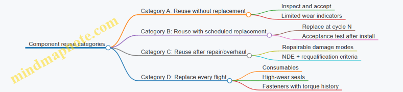
Example: mapping categories to real hardware
- Category A (reuse without replacement): a structural frame that is inspected with NDE and has damage tolerance margins.
- Category B (reuse with scheduled replacement): a valve assembly replaced every 5 flights due to measured erosion.
- Category C (reuse after repair/overhaul): a landing leg that can be repaired after a scrape-through event, but only after specific NDE and dimensional checks.
- Category D (replace every flight): certain gaskets, pyrotechnic initiators, or items with single-use safety assumptions.
This classification turns “reusable” into a set of repeatable operations.
Define the scope in terms of interfaces
Reusability lives at interfaces: mechanical, electrical, software, and operational.
Mechanical interfaces
- Connector mating surfaces and alignment features
- Fastener torque history and replacement rules
- Landing interface geometry and wear limits
Electrical interfaces
- Sensor calibration assumptions after removal/reinstallation
- Harness routing and connector inspection criteria
Software interfaces
- Flight software versioning and verification scope
- GN&C parameter sets tied to stage configuration
Operational interfaces
- Turnaround procedures that define what must be done before the next flight
- Acceptance test boundaries that decide whether a component returns to service
Example: interface-driven scope
If you remove an engine for refurbishment, you need to define what “same engine” means. Is it the same serial number? The same assembly? The same calibration constants? If you don’t specify this, you can’t reliably connect post-flight inspection results to next-flight performance.
Use a scope matrix to prevent gaps
A scope matrix makes it hard to miss a stage/component/mission combination.
Example scope matrix (starter template)
| Level | Item | Reuse decision | Life/limit basis | Post-flight action | Mission set coverage |
|---|---|---|---|---|---|
| Stage | Booster | Reuse | Landing load spectrum + thermal model | Inspect + NDE + acceptance test | Same landing zone + entry mode |
| Propulsion | Engine | Reuse | Hot-fire duty cycles | Valve replacement at cycle N | Same throttle profile family |
| Structure | Tank | Reuse | Damage tolerance + fatigue | Visual + NDE + leak check | Same ascent loads |
| Avionics | GN&C computer | Reuse | Functional test | Bench test + software regression | Same sensor suite |
| TPS | Reentry surface | Reuse with repair | Heat damage thresholds | Inspect + replace damaged panels | Same heating regime |
The matrix forces you to state assumptions. If a column is blank, it’s a sign the scope is not actually defined.
Common scope mistakes (and how to avoid them)
- Scope defined by parts only: you reuse a part, but you don’t define inspection and acceptance. Fix by adding post-flight actions and limits.
- Scope defined by one mission: you assume the same loads always apply. Fix by defining a mission set and mapping it to load drivers.
- Scope defined by “maximum reuse” only: you state a high number of flights without specifying what happens at intermediate cycles. Fix by defining replacement/repair categories and cycle-based actions.
- Scope defined without interfaces: you can’t reproduce the same configuration. Fix by specifying mechanical/electrical/software operational interfaces.
A practical checklist to close the loop
Before moving to architecture and life modeling, confirm you have:
- A one-paragraph scope statement (what, how many, maintenance level, mission set)
- A stage boundary definition (what is recovered vs not)
- A component reuse category for each major subsystem
- A scope matrix with no empty “post-flight action” or “mission coverage” fields
- Interface definitions that connect inspection/repair to next-flight acceptance
When these pieces are in place, the rest of the design work becomes less about arguing what “reusable” means and more about engineering the details that make it repeatable.
1.2 Map Mission Requirements to Reuse Constraints and Interfaces
Mission requirements don’t just tell you what to deliver; they also tell you what you must be able to reuse without surprises. The goal of mapping mission requirements to reuse constraints and interfaces is to turn “we need X” into “we can reuse Y only if interface Z behaves like this, every time.”
Step 1: Start with mission requirements that actually drive reuse
Not every requirement matters for reusability. Focus on the ones that change the hardware’s stress, environment, and inspection burden.
Typical mission requirement categories that strongly affect reuse:
- Performance envelope: payload mass, ascent trajectory, entry corridor, landing accuracy.
- Environment: max dynamic pressure, heating rate, vibration levels, acoustic loads.
- Operations: launch cadence, turnaround time, crew/robot handling constraints.
- Safety and reliability: abort modes, probability targets, fault containment.
- Interfaces: payload electrical/thermal/mechanical, vehicle-to-ground comms, ground support equipment (GSE) hookups.
Concrete example: Suppose the mission requires a landing within ±50 m and a turnaround of 72 hours. Those two requirements immediately constrain guidance accuracy, landing loads, inspection scope, and the availability of test equipment and spare parts.
Step 2: Convert each mission requirement into “reuse-relevant” constraints
For each requirement, ask: what reuse failure mode does this requirement make more likely?
A practical way to do this is to create a constraint statement with three parts:
- What must be preserved across flights (geometry, material properties, calibration state).
- What must be bounded (loads, temperatures, cycles, contamination, wear).
- How it must be verified (inspection method, test, acceptance criteria).
Example mapping table (condensed):
| Mission requirement | Reuse constraint (preserve/bound/verify) | Reuse interface impact |
|---|---|---|
| Entry corridor heating within limits | Preserve TPS integrity; bound peak heat flux and cumulative ablation; verify via inspection + thermal model correlation | TPS inspection access, sensor placement, data products format |
| Landing accuracy ±50 m | Preserve landing gear alignment; bound shock/side-load; verify via post-landing metrology | Mechanical datum interfaces, GNC calibration procedure |
| Turnaround ≤72 hours | Preserve readiness state; bound time for checkout and repairs; verify via health-check checklist | Software data schema, BIT (built-in test) outputs, GSE workflow |
| Payload electrical interface stable | Preserve avionics calibration and power quality; bound noise and timing drift; verify via end-to-end test | Payload connector pinout, harness routing, software timing interface |
Notice how the reuse constraint includes verification. Without that, you only have a hope, not a requirement.
Step 3: Identify the interfaces that carry reuse risk
Interfaces are where assumptions leak. For reusability, the risky interfaces are the ones that change between flights or depend on inspection/repair.
Common reuse-sensitive interfaces:
- Mechanical datums and mounting interfaces: where alignment is established for engines, landing gear, TPS panels, and payload adapters.
- Electrical harnesses and connectors: where wear, fretting, and pin damage can accumulate.
- Software data products: where health metrics, calibration constants, and fault logs must be consistent.
- Thermal interfaces: where insulation condition or contact resistance changes.
- GNC interfaces: where sensor calibration and control law parameters must match the current hardware state.
- Ground support interfaces: where procedures and tooling determine how quickly you can return to flight.
Concrete example: If the mission requires a tight landing corridor, then the interface between post-flight metrology and GNC calibration becomes critical. If the metrology output format changes, or the calibration script expects different units, you can lose accuracy even when the hardware is physically fine.
Step 4: Use a mind map to keep the mapping coherent
This mind map organizes the mapping logic so you can trace from mission requirement to constraint to interface.
Mind map: Mapping mission requirements to reuse constraints and interfaces
Step 5: Build traceability that engineers can actually use
A traceability artifact should answer four questions quickly:
- Which mission requirement drove this reuse constraint?
- What interface must be controlled to satisfy the constraint?
- What verification evidence proves compliance?
- What changes would invalidate the assumption?
A lightweight template that works well in early design reviews:
Requirement ID: MR-____
Mission statement: ______________________

Reuse constraint:
- Preserve: ____________________________
- Bound: _______________________________
- Verify: ______________________________

Interface(s) to control:
- Mechanical: __________________________
- Electrical/software: _________________
- Ground/GSE: _________________________

Verification evidence:
- Inspection: __________________________
- Test/analysis: _______________________
- Acceptance criteria: ________________

Invalidation triggers:
- Repair scope changes: ________________
- Calibration method changes: _________
- Sensor replacement: _________________
Step 6: Walk through one end-to-end example
Let’s use a realistic chain: landing accuracy.
- Mission requirement: land within ±50 m of target.
- Reuse constraint:
- Preserve: landing gear alignment and sensor mounting geometry.
- Bound: cumulative landing shock and side-load per cycle.
- Verify: post-landing metrology and a calibration check before flight.
- Interfaces:
- Mechanical datums between landing gear and vehicle structure.
- Electrical interface to inertial sensors (connector integrity, harness routing).
- Software interface for metrology inputs (units, coordinate frames, timestamping).
- GSE interface for how the vehicle is positioned during metrology.
- Verification:
- NDE/inspection for structural damage at known stress points.
- Metrology measurement repeatability check.
- End-to-end GNC sanity test using the updated calibration constants.
If any interface is uncontrolled, the reuse constraint becomes hard to prove. For instance, if the GSE positioning reference changes slightly between turnaround cycles, your metrology could be biased. The vehicle would still “pass inspection,” but the calibration would be wrong.
Step 7: Add “interface contracts” to prevent drift
Once you know which interfaces matter, define contracts that specify what must remain true.
Examples of interface contracts that are simple but effective:
- Coordinate frame contract: metrology outputs must declare origin, axes, and units.
- Calibration contract: sensor calibration constants must include validity range and date.
- Connector contract: harnesses must be keyed and serialized so replacements can’t silently swap pinouts.
- Data contract: health-check outputs must follow a fixed schema so ground scripts and flight software interpret them consistently.
A good rule of thumb: if a human could misinterpret the interface, the interface needs a contract.
Step 8: Keep the mapping honest with “assumption checks”
Engineers often assume that because a requirement is met once, it will be met again. Reusability engineering replaces that assumption with explicit checks.
Assumption checks to include during mapping:
- Does the verification method still work after the expected wear/repair?
- Are acceptance criteria tied to measurable quantities, not vague judgments?
- Can the interface be re-established quickly enough to meet turnaround?
- Are there any hidden dependencies on prior flight history?
Concrete example: If a thermal model correlation is tuned using flight data from one configuration, then a repaired TPS panel with different surface roughness might break the correlation. The mapping should either bound that change or require a specific verification step after repair.
Summary
Mapping mission requirements to reuse constraints and interfaces is a traceability exercise with teeth. You take mission needs, translate them into preserve/bound/verify constraints, then identify the interfaces that carry the risk of violating those constraints. When the interface contracts and verification evidence are explicit, reusability stops being a slogan and becomes an engineering system.
1.3 Compare Reuse Modes Using Concrete Example Payload Profiles
Reusability isn’t one thing. It’s a set of design choices that trade hardware life, refurbishment effort, and mission flexibility. A good way to compare reuse modes is to anchor them to payload profiles that stress different parts of the launch system.
Reuse modes you’ll actually see in system trade studies
Below are three common reuse modes engineers compare. They differ in what gets reused, how often, and what must be inspected or repaired between flights.
-
Mode A: Partial reuse (recover and reuse a subset)
- Example: reuse the first stage and its engine set; keep upper stages expendable.
- Typical driver: reduce cost per launch while keeping upper-stage complexity manageable.
-
Mode B: Stage reuse (recover and reuse the same stage multiple times)
- Example: reuse both the first stage and an intermediate stage; uppermost stage may be expendable.
- Typical driver: reduce recurring hardware cost more aggressively, at the expense of more refurbishment scope.
-
Mode C: Fully reusable architecture (multiple stages recovered)
- Example: recover and reuse all major stages that carry the vehicle through the highest-cost segments.
- Typical driver: maximize reuse value, but refurbishment and verification become the center of gravity.
The payload profile determines which mode is easiest to justify.
Mind map: payload profiles mapped to reuse stressors
Example 1: Low-mass LEO rideshare (cadence and schedule dominate)
Payload profile: 1–3 small satellites, modest volume, frequent launches, and a customer expectation that the next flight will happen on time.
Concrete assumptions for comparison (illustrative):
- Target: deliver to a near-circular LEO with small dispersion tolerance.
- Typical constraints: fairing/adapter integration must be repeatable; launch site processing must not become the bottleneck.
Mode A (partial reuse)
- What’s reused: first stage.
- Why it fits: the most expensive part of the vehicle to manufacture repeatedly is often the first-stage propulsion and structure. Reusing it reduces cost while leaving upper-stage integration simpler.
- Where it bites: turnaround operations still depend on first-stage recovery success. If recovery occasionally slips, the schedule impact is concentrated in the part you’re reusing.
Example decision point: If the first-stage refurbishment time has a wide spread (say, sometimes 2 days, sometimes 6), rideshare cadence suffers. Mode A can still work, but the system must treat refurbishment variability as a first-class requirement.
Mode B (stage reuse)
- What’s reused: first stage plus an intermediate stage.
- Why it fits: more hardware cost is reduced per flight.
- Where it bites: refurbishment scope grows. You now have more components that must be inspected, repaired, and reassembled without introducing new variability.
Example decision point: If the intermediate stage requires additional NDE steps that take longer than the schedule buffer, the system may lose the cadence advantage even if hardware cost drops.
Mode C (fully reusable)
- What’s reused: all major stages.
- Why it fits: maximum reuse value.
- Where it bites: the number of “things that can delay the next flight” increases. Even if each inspection is manageable, the combined probability of a schedule-impacting nonconformance rises.
Example decision point: For rideshare, the payload is less sensitive to performance margin than to schedule. If full reuse adds verification steps that occasionally force a hold, the customer experience degrades.
Takeaway for this profile: cadence and turnaround variability favor Mode A or Mode B with tight refurbishment control. Fully reusable can work, but only if refurbishment and verification are engineered to be predictably repeatable.
Example 2: High-mass LEO / constellation deployment (performance margin and structural life matter)
Payload profile: larger payloads, repeated similar trajectories, and a need for consistent performance margins to avoid expensive payload workarounds.
Concrete assumptions:
- The mission requires a narrow propellant margin budget.
- Recovery loads and thermal cycles repeat frequently.
Mode A (partial reuse)
- What’s reused: first stage.
- System effect: performance consistency depends heavily on first-stage engine repeatability and propellant conditioning.
- Structural life: fatigue management is concentrated in the first stage.
Example: If first-stage refurbishment includes replacing a limited set of wear items (e.g., valves or seals) and the remaining structure is inspected against damage tolerance criteria, the system can maintain performance consistency.
Mode B (stage reuse)
- What’s reused: first stage plus intermediate stage.
- System effect: now both stages contribute to performance margin consistency.
- Structural life: fatigue and inspection scope expand.
Example: Suppose the intermediate stage experiences recovery loads that are less severe than the first stage but still nontrivial. The system can still be stable if life limits are set conservatively and inspection coverage is aligned with the failure modes that actually occur.
Mode C (fully reusable)
- What’s reused: all major stages.
- System effect: upper-stage performance consistency becomes part of the reuse story.
- Structural/thermal: more surfaces and subsystems must meet acceptance criteria after multiple cycles.
Example: If upper-stage thermal protection requires frequent refurbishment or conservative replacement, the performance margin budget can become dominated by refurbishment uncertainty rather than propulsion capability.
Takeaway for this profile: performance margin consistency and structural life management favor Mode B when refurbishment scope is controlled, while Mode C requires particularly disciplined acceptance criteria to avoid margin erosion.
Example 3: High-energy transfer (upper-stage sensitivity and mission assurance dominate)
Payload profile: transfer to higher-energy orbits with longer mission phases and tighter upper-stage performance sensitivity.
Mode A (partial reuse)
- What’s reused: first stage only.
- Why it’s attractive: upper-stage mission assurance stays simpler because it’s not reused.
- Where it bites: the first-stage recovery must not introduce integration variability that affects upper-stage ignition conditions.
Example: If the vehicle-to-vehicle interface (stage separation, electrical connectors, propellant conditioning) is not controlled, then even a reused first stage can indirectly affect upper-stage performance.
Mode B (stage reuse)
- What’s reused: first stage plus intermediate stage.
- Why it’s workable: upper-stage remains expendable, so the most mission-sensitive segment is not reused.
- Where it bites: intermediate-stage avionics and thermal/structural elements must be verified to the same level of confidence as the first stage.
Example: If intermediate-stage guidance software is reused, regression testing must cover the exact configuration changes introduced by refurbishment.
Mode C (fully reusable)
- What’s reused: upper stage too.
- Why it’s hardest: mission assurance now includes reused elements that directly affect high-energy performance.
Example: If the upper stage’s thermal protection or structural elements have acceptance criteria that are difficult to satisfy consistently, then the system spends more time in verification and less time in flying.
Takeaway for this profile: high-energy missions generally favor Mode A or Mode B, because keeping the most mission-sensitive stage expendable reduces the verification burden.
A compact comparison table (what changes across modes)
| Payload profile | Primary success factor | Mode A (partial reuse) | Mode B (stage reuse) | Mode C (fully reusable) |
|---|---|---|---|---|
| Low-mass LEO rideshare | Turnaround predictability | Good fit if first-stage refurbishment is bounded | Works if intermediate refurbishment doesn’t add schedule variance | Risky if combined inspections create holds |
| High-mass LEO / constellations | Performance margin consistency + life | Stable if first-stage life limits are enforced | Strong if both reused stages have disciplined acceptance | Harder if upper-stage refurbishment uncertainty grows |
| High-energy transfer | Mission assurance + upper-stage sensitivity | Often simplest assurance path | Balanced if upper stage stays expendable | Most verification-heavy |
Practical best practice: compare modes using “constraint budgets”
When you compare reuse modes, don’t start with cost. Start with budgets that reuse affects directly:
- Turnaround budget: maximum allowable refurbishment time and its variability.
- Verification budget: number and duration of checks required to reach flight readiness.
- Life/acceptance budget: how many cycles before inspection thresholds or replacements.
- Interface budget: how refurbishment affects stage separation, electrical connections, and propellant conditioning.
Example workflow:
- Pick a payload profile.
- Identify which constraints are tightest (schedule, margin, assurance).
- For each reuse mode, list the added refurbishment and verification steps.
- Score each mode against the constraint budgets using the same rubric.
This approach keeps the comparison grounded: you’re not arguing about “how reusable” a system is; you’re quantifying whether reuse helps the mission you’re actually flying.
1.4 Establish Success Metrics for Reuse Reliability, Turnaround, and Cost
A reusable launch system is only “reusable” if it reliably survives repeated use, can be processed again without heroic effort, and actually reduces total cost per mission. Success metrics turn those three ideas into numbers teams can plan around, measure against, and improve.
Reuse reliability: measure what matters for the next flight
Start by defining the unit of reuse you’re measuring. It might be a stage, an engine, a landing system, or a thermal protection set. Then define the failure modes that prevent reuse from being accepted for the next mission.
Recommended reliability metrics (pick a few, not all):
-
Reuse acceptance yield (RAY): fraction of reused items that pass post-flight inspection and are cleared for the next flight.
- Example: If 8 returned booster cores are inspected and 6 are cleared, then RAY = 6/8 = 75%.
- Why it’s useful: it captures inspection reality, not just component physics.
-
Flight readiness probability (FRP): probability that an item is ready by the scheduled processing start date.
- Example: If a core is cleared but a missing part delays it, FRP is lower than RAY.
- Why it’s useful: it connects reliability to schedule.
-
Life-cycle failure rate (LCFR): failures per reused cycle for life-limited or high-consequence items.
- Example: If a valve set experiences 1 failure across 30 reused cycles, LCFR = 1/30 ≈ 3.3% per cycle.
- Why it’s useful: it supports life management and spares planning.
-
Time-to-clear (TTC): distribution of days from landing to “cleared for processing.”
- Example: If typical clearance takes 5 days but some cases take 18, the mean hides risk; track percentiles (P90 is especially telling).
A simple reliability scorecard layout
| Metric | Definition | Target example | What it catches |
|---|---|---|---|
| RAY | Cleared / returned | ≥ 90% | inspection and repair reality |
| FRP | Ready by schedule start | ≥ 95% | logistics and rework delays |
| LCFR | Failures / reused cycle | ≤ 2% | life-limited degradation |
| TTC (P90) | 90th percentile clearance days | ≤ 7 days | worst-case processing drag |
Turnaround: measure throughput and the “last mile”
Turnaround success is not just average processing time. A reusable system is a queueing system: you care about throughput, variability, and the probability of missing a processing window.
Recommended turnaround metrics:
-
Processing time (PT): total calendar time from landing to “ready for integration.”
- Example: Core lands Monday, integration starts Friday next week → PT = 9 calendar days.
-
Critical-path duration (CPD): time spent on the longest dependency chain (often inspection → NDE → repair → reassembly → verification).
- Example: If NDE results drive the schedule, CPD will track that better than PT.
-
Turnaround yield (TAY): fraction of items that complete turnaround within the planned window.
- Example: If 10 cores are scheduled for a 10-day window and 8 finish within it, TAY = 80%.
-
Rework rate (RR): fraction of items requiring repeat work due to inspection findings or verification failures.
- Example: If 3 of 10 cores require a second NDE/repair cycle, RR = 30%.
Why variability deserves a metric
If you only track mean PT, a system with occasional long delays can still look “fine” until a tight launch cadence exposes it. Percentiles (P80/P90) and window-miss probability are the practical tools.
Window-miss probability example
Let the planned processing window be (W) days and actual processing time be (T). Define: \[ P_{miss} = P(T > W) \] If you observe \(P_{miss} = 0.15\), then in a 10-flight campaign you should expect about 1–2 misses, even if the average time looks acceptable.
Cost: separate cost drivers from cost outcomes
Cost metrics should reflect the full cost per mission, but also separate the parts you can control.
Recommended cost metrics:
-
Cost per reused cycle (CPRC): cost to refurbish and process a reused item for one additional flight.
- Example: If refurbishment labor, materials, test time, and overhead sum to $12M per core flight, CPRC = $12M.
-
Marginal cost per mission (MCM): incremental cost of flying with reuse versus flying with new hardware.
- Example: If a new core mission costs $60M and a reuse mission costs $40M, then MCM = $-20M (a savings of $20M).
-
Cost of nonconformance (CONC): cost attributable to rework, scrapped items, and schedule penalties.
- Example: If 2 of 10 cores are scrapped after inspection, the scrap cost and re-test cost should be tracked separately from routine refurbishment.
-
Unit cost of readiness (UCR): cost divided by probability of being ready on time.
- Example: If expected readiness probability is 0.9 and the average processing cost is $12M, then UCR ≈ $13.3M per “effective ready unit.”
A practical cost decomposition
Track cost in buckets that map to engineering decisions:
- Hardware refurbishment (parts, repairs, coatings)
- Verification and testing (NDE, hot-fire equivalents, software regression)
- Operations and labor (processing labor, shifts, tooling)
- Schedule risk costs (expedites, overtime, missed windows)
This prevents a common failure mode: teams reduce one bucket (say, labor) while increasing another (say, rework), and the total cost per mission quietly rises.
Mind map: metrics that connect engineering to operations
Example: turning metrics into actionable targets
Suppose you’re tracking a reusable booster core.
- Observed RAY over the last 6 flights: 7 cleared out of 8 returned → RAY = 87.5%.
- Observed TTC (P90): 12 days, while your integration start window assumes 7 days.
- Observed TAY: 5 of 6 cores finished within the 10-day window → TAY = 83%.
- Cost buckets show rework-heavy NDE and repair as the largest contributor to CONC.
A reasonable metric-driven improvement plan is to set targets that address the bottleneck:
- Raise RAY to ≥ 92% by tightening inspection acceptance criteria and improving repair repeatability.
- Reduce TTC (P90) to ≤ 8 days by standardizing NDE workflows and pre-positioning common repair kits.
- Increase TAY to ≥ 90% by reducing RR and shortening CPD.
- Reduce CONC by attacking the top two rework causes, not by cutting routine verification.
The key is that each metric has a clear “lever” behind it. If a metric improves but nothing operational changes, it’s probably measuring the wrong thing—or measuring it too late.
Closing the loop: define measurement cadence and ownership
Metrics only help if they’re measured consistently and owned by teams with authority to act. Set a cadence (per flight, per refurbishment cycle, per campaign) and tie each metric to a responsible function: engineering for LCFR, quality/NDE for RAY and TTC, and operations for PT/CPD/TAY. When the numbers move, the system learns; when they don’t, you know exactly where the friction lives.
2. System Architecture Choices That Enable Reuse
2.1 Select Reusable Stage Boundaries and Propulsion Partitioning
Reusable launch systems live or die by boundaries: where one “unit” ends and another begins, and which propulsion elements are expected to survive multiple flights. The goal is not just reusability in principle; it’s reusability that survives real constraints like mass growth, inspection time, and the fact that engines and structures don’t age politely.
Start with the stage boundary question
A reusable stage boundary is the interface where you decide which hardware must be recovered, refurbished, and flown again. That decision should be driven by three practical factors:
- Energy and environment exposure: The stage that experiences the highest thermal and mechanical stress usually needs the most careful life management.
- Mass and propellant partitioning: Propellant mass affects both performance and the size of the recovered structure.
- Operational turnaround: The boundary determines what must be inspected, repaired, and reassembled between flights.
A useful way to reason about this is to treat the boundary as a “life-management contract.” If the contract says the stage will be recovered, then the propulsion and structure on that stage must be designed for repeated cycles, including inspection access and repair paths.
Boundary selection patterns (and when they work)
Most designs converge on one of a few boundary patterns. You don’t need to copy any specific architecture, but you do need to understand the trade.
Pattern A: Recover the first stage; keep upper stage expendable
Why it’s common: The first stage does the heavy lifting through the densest atmosphere and typically has the largest recovery benefit. The upper stage can be simpler if it’s not expected to return.
What to watch: If you partition propulsion so that only the first stage engines are reusable, you must ensure the upper stage has enough performance margin without relying on “borrowed” thrust from reusable hardware.
Example: Suppose the mission requires a 2nd-stage burn to reach a specific orbit. If the upper stage is expendable, you can size its engines for one duty cycle with less life margin. Meanwhile, the first stage engines are sized with a life budget that includes multiple hot-fire cycles plus the additional thermal soak and cooldown periods associated with recovery.
Pattern B: Recover both stages, but with different reuse levels
Why it’s attractive: It can reduce total propellant mass per flight by allowing more of the vehicle to be reused.
What to watch: Turnaround complexity rises quickly because you now inspect and repair more hardware. Also, the upper stage experiences different loads and thermal environments than the first stage.
Example: A design might recover the upper stage but accept that only certain components are reused. For instance, you might reuse the stage structure and avionics while replacing the most life-limited propulsion elements after each flight. That’s still “reusable stage” behavior, but with a clear partition of what is truly flight-to-flight.
Pattern C: Recover only the propulsion module; keep the stage structure expendable
Why it exists: Sometimes the propulsion module is the expensive, life-limited element, and the structure is easier to replace.
What to watch: This can create integration friction: you still need to mate the recovered propulsion module to a new structure reliably, with consistent alignment and interface quality.
Example: If you recover a reusable engine section with its turbomachinery and control valves, you must ensure the new structure provides repeatable mounting geometry and propellant feed alignment. Otherwise, the engine’s performance and vibration environment change between flights, which can undermine life assumptions.
Propulsion partitioning: decide what is reusable, not just where
Propulsion partitioning is the split between reusable and replaceable propulsion elements across the stage boundary. It’s tempting to treat “engine reuse” as a single yes/no decision, but real systems partition by subsystems.
A practical partitioning approach is to list propulsion subsystems and assign them one of three reuse levels:
- Flight-to-flight reusable (designed for repeated cycles with inspection/repair)
- Condition-based reusable (reused if health metrics pass)
- Replace-after-use (treated as consumable hardware)
Example partition for a reusable first stage
Consider a first stage with multiple engines.
- Reusable: main combustion chamber assembly, turbopump (with life-limited margins), engine controller hardware
- Condition-based: certain valves and seals that are sensitive to wear and thermal cycling
- Replace-after-use: specific high-wear components like igniters or selected gaskets, depending on inspection findings
The key is that the stage boundary and propulsion partitioning must agree. If the boundary says the stage is recovered, but the propulsion partitioning effectively replaces the entire engine after every flight, you’ve shifted cost and schedule without gaining the benefits you expected.
Interface logic: make the boundary “mechanically honest”
A stage boundary is not just a line on a block diagram. It’s a set of mechanical, thermal, electrical, and fluid interfaces that must behave consistently across flights.
Mechanical interfaces
Reusable boundaries need repeatable alignment. Even small changes in mounting geometry can alter vibration modes and propellant feed behavior.
Best practice: Use a repeatable kinematic mounting concept (e.g., defined hardpoints plus controlled compliance) so that reassembly doesn’t depend on “whoever tightened it last time.”
Example: If the engine mount uses multiple bolts, define torque procedures and inspection checks that verify preload and seating. Then design the mount so that any residual variation stays within the engine’s allowable misalignment.
Fluid interfaces
Propellant feed lines and quick-disconnects are frequent sources of turnaround delays.
Best practice: Partition plumbing so that the most failure-prone connections are either:
- on the replaceable side of the boundary, or
- designed for rapid inspection with clear leak-check access.
Example: If you use quick-disconnects at the stage boundary, ensure the leak-check procedure can be performed without disassembling additional layers. Otherwise, the boundary becomes a schedule trap.
Electrical and avionics interfaces
Reusable stages often reuse avionics, but the boundary still needs robust connector strategy.
Best practice: Define connector families and pinouts that remain stable across flights. If you must change wiring, treat it as a configuration-managed change with verification.
Example: If the stage boundary includes a harness that routes power and sensor signals, keep the harness length and routing consistent so that vibration and thermal exposure remain within the tested envelope.
Mind map: boundary and propulsion partitioning
A concrete decision workflow (engineers actually use this)
- List candidate boundaries (e.g., recover first stage only; recover both; recover propulsion module only).
- For each boundary, assign propulsion reuse levels by subsystem.
- Check interface feasibility: can you reassemble quickly and repeatably, with inspection access?
- Validate life assumptions against the boundary: if the stage is recovered, include recovery-related thermal and mechanical events in the life budget.
- Confirm performance consistency: if some propulsion elements are replaced, ensure the replacement hardware has verified performance spread.
Example: comparing two boundary options
-
Option 1: Recover first stage; upper stage expendable.
- Propulsion partitioning: first-stage engines flight-to-flight reusable; upper-stage engines replace-after-use.
- Interface focus: stage boundary plumbing and engine mount repeatability.
- Turnaround: dominated by first-stage inspection and reassembly.
-
Option 2: Recover both stages.
- Propulsion partitioning: both stages condition-based reusable.
- Interface focus: additional boundary on upper stage, plus more connectors and plumbing.
- Turnaround: inspection and repair time increases because more hardware must pass reuse criteria.
The “best” option is the one where the interface and life-management work is consistent with the operational plan. If turnaround time is dominated by boundary inspections, you can’t fix that later with better optimism.
Common pitfalls
- Boundary chosen for performance, not for inspection: If the boundary hides critical interfaces, reuse becomes slow.
- Propulsion partitioning that contradicts the boundary: A recovered stage that effectively replaces all propulsion hardware each time is usually a cost and schedule mismatch.
- Unmanaged configuration drift: If connector pinouts, harness routing, or mounting procedures change without controlled verification, reuse assumptions stop being true.
Bottom line
Selecting reusable stage boundaries and propulsion partitioning is a coupled design problem. The boundary defines what must survive recovery and refurbishment; propulsion partitioning defines what must survive repeated duty cycles. When those two decisions align with interface repeatability and inspection practicality, reusability becomes an engineering property rather than a hope.
2.2 Design for Recoverability With Clear Landing and Retrieval Concepts
Recoverability is not a single subsystem requirement; it’s a chain of decisions that starts at the stage boundary and ends at the last bolt on the pad. If you want reuse to be more than a spreadsheet promise, design the vehicle so that landing and retrieval are predictable, inspectable, and repairable.
Start with the recovery “contract”
A useful way to frame recoverability is to write a contract between flight hardware and ground operations. The contract states what the vehicle will deliver after flight and what the ground system will do with it.
Include these items explicitly:
- Landing state definition: where the vehicle lands, what attitude it should be in, and what tolerances matter for safe handling.
- Post-landing power and data: whether the vehicle can provide health data after touchdown and how long it can do so.
- Physical access plan: which surfaces and fasteners must be reachable without special tools or hazardous procedures.
- Inspection and repair interfaces: where sensors, ports, and access panels are located so that inspection does not require disassembly.
Example: If your recovery plan assumes you can inspect a tank weld visually, then the design must keep that weld accessible after landing. If the weld is buried under a fairing that always needs removal, your inspection time becomes a variable you didn’t budget.
Choose a landing concept that matches your retrieval reality
Landing concepts usually fall into a few patterns: runway landing, barge or platform landing, parachute-assisted splashdown, or controlled landing with landing legs. The vehicle design should reflect the retrieval method’s constraints.
Key design-to-retrieval links:
- Landing gear geometry and load paths: retrieval teams care about where lifting forces can be applied without damaging structure.
- Touchdown attitude and center-of-mass location: if the vehicle lands “upright enough,” you reduce the need for heavy repositioning.
- Propellant and residuals management: retrieval operations need predictable venting, draining, and safe handling.
Example: A stage that lands on legs but leaves residual propellant in low points can force ground teams to wait for settling and venting. That turns a quick turnaround into a waiting game. Design the propellant system so residuals drain to known locations.
Design for safe handling: lifting, towing, and restraint
Recovery operations often require moving a landed stage from the landing site to a processing area. That movement must not rely on “careful humans” as the primary safety mechanism.
Practical best practices:
- Define lift points and their allowable loads in the structural design. Treat them like interfaces, not afterthoughts.
- Provide restraint features for transport (e.g., hardpoints for straps) so the vehicle can’t shift during towing.
- Avoid fragile external features at lift-contact locations. A cover that looks sturdy can still crack under strap pressure.
Example: Suppose you add a sensor pod on the side for post-flight diagnostics. If retrieval straps pass near it, the pod becomes a damage hotspot. Either relocate it or design it to survive strap contact and inspection.
Make the landing system “inspectable by design”
Landing hardware is where you often get the most wear: legs, shock absorbers, and any mechanisms that deploy or lock. Design these elements so that the inspection plan is straightforward.
Include:
- Clear wear surfaces: identify where abrasion, fretting, or impact damage is likely.
- Access panels or removable covers: allow NDI (nondestructive inspection) without removing major assemblies.
- Mechanical indicators: simple visual or sensor-based indicators can confirm whether a mechanism deployed and locked.
Example: If landing legs deploy via a latch, add a mechanical position indicator visible after landing. Ground teams can quickly confirm latch state before applying any lifting loads.
Define touchdown tolerances that protect structure and operations
Touchdown is a coupled event: vehicle dynamics, landing gear response, and ground constraints. You need tolerances that are meaningful for both structural safety and operational handling.
A good approach is to define three layers of tolerances:
- Structural limits: maximum loads and deflections the stage can tolerate.
- Operational limits: conditions under which ground handling is safe and efficient.
- Inspection limits: thresholds beyond which inspection becomes extensive.
Example: If the stage can structurally survive a higher landing load but only if you remove a panel to inspect a specific region, then that higher load should be treated as an operational limit, not just a structural one.
Plan for residual energy and propellant safety
Recoverability requires managing residual energy: pressure, temperature, and electrical charge. Ground operations should not have to guess.
Design actions that help:
- Predictable venting paths for tanks and lines so pressure decays in a controlled manner.
- Known electrical discharge behavior for batteries and capacitors.
- Thermal considerations so hot surfaces cool to safe handling temperatures within a defined window.
Example: If a stage uses a battery for post-landing telemetry, specify the discharge strategy so that the battery is safe to disconnect at the start of the inspection window.
Build retrieval-friendly geometry and clearances
Retrieval is easier when the vehicle’s external geometry supports tooling and clearance.
Common design-to-retrieval practices:
- Tooling clearance envelopes around access points.
- Avoidance of snag-prone protrusions near areas where cranes or lift frames operate.
- Consistent datum surfaces so alignment during lifting is repeatable.
Example: If you expect to use a lift frame with fixed attachment points, design those points with consistent geometry across reused hardware. If tolerances stack differently after refurbishment, the lift frame becomes a source of delays.
Use a “recovery sequence” to drive requirements
Write the recovery sequence as a step-by-step process and let it generate requirements. Each step should have an input state and an output state.
A simple sequence template:
- Post-landing stabilization (attitude and power state)
- Safe-to-handle verification (pressure, temperature, electrical)
- Initial inspection (visual checks and indicator verification)
- NDI/repair access (open panels, expose inspection regions)
- Refurbishment and reassembly
- Pre-flight readiness checks
Example: If step 3 includes verifying a latch indicator, then the indicator must be visible without removing covers. If it’s not visible, you’ve turned a 10-minute check into a multi-hour teardown.
Mind map: landing and retrieval concept design
Concrete example: designing for a legged landing and crane retrieval
Imagine a reusable stage that lands on four legs and is retrieved by crane.
Design choices driven by recovery:
- Legs include inspection access: each leg has a removable cover over the shock strut attachment so NDI can be performed without detaching the leg.
- Lift points are integrated into the primary structure: crane attachment points connect to load-bearing members, not to fairings or covers.
- Touchdown attitude is controlled: guidance targets a small pitch/roll window so the stage rests within a crane lift envelope.
- Residual propellant drains to known locations: vent and drain valves are positioned so ground teams can connect hoses without reaching into tight gaps.
Operational payoff: the crane can attach using fixed geometry, the first inspection can confirm leg deployment via indicators, and the team can start NDI within the planned window because residual energy is predictable.
Common failure modes (and how to design them out)
- “We can retrieve it, but it’s slow.” Fix by designing lift points and access panels so the recovery sequence doesn’t require ad-hoc work.
- “It lands fine, but inspection is painful.” Fix by placing inspection regions where they remain reachable after landing.
- “Ground teams wait for safety.” Fix by specifying venting, discharge, and thermal cooling behavior so safe-to-handle timing is deterministic.
Recoverability is a system-level property. When landing and retrieval concepts are treated as first-class design drivers, the vehicle becomes easier to handle, easier to inspect, and less dependent on heroic troubleshooting.
2.3 Choose Guidance, Navigation, and Control Strategies for Multiple Flights
Reusable launch vehicles don’t just repeat the same mission; they repeat the same problems with slightly different starting conditions. Guidance, Navigation, and Control (GNC) strategies for multiple flights must therefore be robust to hardware wear, sensor drift, and changing vehicle health—while still meeting tight performance and safety requirements.
Start with what changes between flights
A reusable system typically varies across flights in ways that matter to control:
- Mass properties: residual propellant, insulation condition, and repaired structures shift center of mass and inertia.
- Aerodynamic state: surface condition, hinge friction, and fairing separation timing can change drag and control effectiveness.
- Sensor behavior: accelerometer bias, gyro scale factors, and GNSS reception quality vary with temperature history and mounting stress.
- Actuator limits: valve response, gimbal friction, and thruster performance degrade or recover depending on maintenance actions.
A practical best practice is to define a flight-to-flight variation budget for each GNC-relevant quantity (mass, thrust, drag, sensor bias, actuator lag). Then you design the estimator and controller to tolerate that budget without “fighting” the vehicle.
Guidance architecture: reuse-friendly trajectories and modes
For multiple flights, guidance should be structured around modes that match the vehicle’s operational phases and the information available in each phase.
A common approach is:
- Ascent guidance: track a time-parameterized or state-parameterized reference that accounts for thrust and mass changes.
- Entry/reentry guidance (if applicable): use a guidance law that can handle large uncertainties in atmospheric density and vehicle aerodynamics.
- Terminal guidance: switch to a guidance mode that prioritizes landing constraints (velocity, attitude, and lateral position).
The key reuse practice is to make mode transitions deterministic and testable. For example, define explicit triggers such as “switch when dynamic pressure exceeds X and attitude error is below Y” rather than relying on a single time-based switch.
Example: mode switching for terminal landing
Suppose the terminal phase uses a guidance law that assumes near-stable attitude control authority. A robust strategy is to require both:
- Attitude convergence: \[ |\theta_{err}| < \theta_{max} \]
- Sufficient control authority: estimated control effectiveness \(\hat{B}\) above a threshold.
If either condition fails, the system stays in a “recovery” guidance mode that uses gentler commands until the assumptions are valid.
Navigation strategy: estimators that survive sensor and health changes
Navigation for reusable vehicles should not assume perfect sensors every flight. Instead, build an estimator that can handle:
- bias drift,
- occasional measurement dropouts,
- changing process noise due to actuator or model changes.
A typical reusable-friendly navigation stack includes:
- State estimator (e.g., extended Kalman filter or similar): fuses IMU, GNSS (when available), and sometimes radar/altimeter.
- Health-aware noise tuning: adjust measurement noise \(R\) and process noise \(Q\) based on sensor status.
- Model adaptation hooks: allow thrust and drag parameters to be updated from recent data.
Example: bias-aware inertial navigation
If an accelerometer bias \(b_a\) drifts, the estimator can treat \(b_a\) as a slowly varying state with a random-walk model: \[ \dot{b}_a = w_b, \quad w_b \sim \mathcal{N}(0, \sigma_b^2) \] Then, when GNSS updates are available, the estimator corrects the bias. When GNSS is degraded, the bias uncertainty grows in a controlled way rather than silently producing overconfident state estimates.
Control strategy: controllers that tolerate changing plant dynamics
Controllers for reusable vehicles must handle changes in:
- actuator saturation and rate limits,
- effective thrust and gimbal authority,
- aerodynamic control effectiveness.
A robust pattern is to separate control into layers:
- Inner loop: fast attitude stabilization using measured or estimated angular rates.
- Outer loop: slower guidance-to-control translation producing commanded accelerations or thrust vector angles.
This separation helps reuse because the inner loop can remain stable across a range of plant conditions, while the outer loop adapts to guidance demands.
Example: actuator saturation handling without integrator windup
If a gimbal command saturates, an integrator can accumulate error and cause overshoot when the actuator recovers. A reusable-friendly practice is to implement anti-windup logic tied to saturation detection.
A simple conceptual rule:
- If commanded control \(u_c\) exceeds limits, apply the saturated output \(u_s\) to the plant model and freeze or back-calculate the integrator state.
This prevents “remembering” the impossible command across the rest of the flight.
Reuse-aware robustness: design around uncertainty, not around perfect models
For multiple flights, the controller should be designed with explicit uncertainty bounds. Two practical mechanisms:
- Gain scheduling: adjust controller gains based on estimated dynamic pressure, propellant level, or actuator temperature.
- Robust margins: ensure stability and performance for the worst-case combination of thrust and aerodynamic uncertainty within the variation budget.
Example: gain scheduling by dynamic pressure
If aerodynamic control effectiveness scales with dynamic pressure \(q\), then the controller can schedule gains based on \(q\):
- high \(q\): stronger authority, tighter attitude error targets,
- low \(q\): reduced authority, more conservative commands.
This reduces the chance that the controller assumes authority that isn’t there.
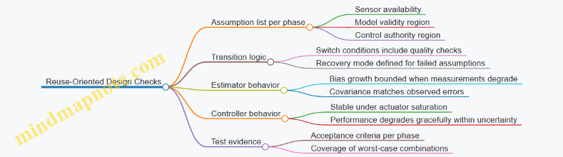
Verification strategy: prove the reuse assumptions, not just the nominal case
To make GNC reusable, verification should include:
- Monte Carlo runs with sensor bias drift and actuator response variations,
- fault injection for measurement dropouts and stuck actuators,
- hardware-in-the-loop tests that use the same estimator and controller code as flight.
A good reuse practice is to define acceptance criteria per phase:
- maximum attitude error,
- maximum velocity error at phase boundaries,
- constraint violations (gimbal limits, thrust limits, landing velocity windows).
Mind maps
Mind Map: GNC Strategy for Multiple Flights
Mind Map: Reuse-Oriented Design Checks
A compact end-to-end example (how the pieces fit)
Consider a reusable stage that performs ascent, then a terminal landing burn.
- Guidance defines three modes: ascent tracking, coast/entry (if present), and terminal landing. Terminal mode activates only when attitude error is small and estimated control effectiveness is above a threshold.
- Navigation runs an estimator that treats accelerometer bias as a state. When GNSS is available, it corrects bias; when GNSS degrades, covariance grows and the controller uses the estimator’s uncertainty rather than pretending certainty.
- Control uses an inner attitude loop with gain scheduling based on dynamic pressure and an outer loop that commands accelerations consistent with thrust and gimbal limits. Anti-windup prevents integrator buildup during saturation.
- Verification includes Monte Carlo runs with thrust scaling, drag variation, sensor bias drift, and actuator response lag. Acceptance criteria are checked at mode boundaries and at landing constraints.
The result is not a single “perfect” controller. It’s a set of design choices that keep the system coherent when the vehicle is not identical to the previous flight—which, for reusable hardware, is the normal case.
2.4 Integrate Reuse-Aware Avionics and Health Monitoring From Day One
Reusability is not only a mechanical design problem; it’s also an information problem. If the avionics and health monitoring system treats every flight like a brand-new vehicle, you’ll either miss useful wear signals or drown in false alarms. Reuse-aware avionics aims for a simple outcome: the system should know what it has seen before, what it did to the hardware, and what that implies for the next flight.
What “reuse-aware” means in avionics terms
A reuse-aware avionics architecture includes three capabilities:
- Flight-to-flight state continuity: the system carries forward relevant hardware state (e.g., engine cycles, valve actuations, structural inspection results) into the next mission’s decision logic.
- Contextual health monitoring: thresholds and diagnostics adapt to the component’s history and expected operating profile, not just generic limits.
- Actionable outputs: health results drive concrete ground actions (inspect, replace, derate, or clear) with traceable evidence.
A practical way to keep this from becoming a vague goal is to define “decision points” early. For example: “If turbopump bearing vibration exceeds X during ascent, then ground processing must perform Y inspection before the next flight.” The avionics and health monitoring design should directly support those decisions.
Mind map: reuse-aware avionics and health monitoring
Mind Map: Reuse-Aware Avionics & Health Monitoring
Design the data model before you design the algorithms
Health monitoring fails most often at the interface between “what happened” and “what the ground team can use.” Start by defining a minimal, stable data model that travels with the hardware.
A good baseline includes:
- Hardware identity: unique IDs for each life-limited component (engine, turbopump, major valves, actuators).
- Usage counters: cycles and event counts that correlate with wear mechanisms.
- Operational context: key conditions during each flight segment (e.g., peak chamber pressure, max valve duty, ascent duration).
- Health evidence: raw or reduced sensor products tied to events (e.g., vibration spectra around throttle transitions).
- Decision outcomes: what actions were taken after the flight (inspect/replace/clear) and why.
If you skip this and jump straight to diagnostics, you’ll end up with clever algorithms that produce results no one can interpret consistently across flights.
Build health monitoring around “segment-aware” expectations
A reusable vehicle doesn’t just repeat a mission; it repeats segments with different loads and different sensor observability. Segment-aware monitoring means the avionics knows which phase it’s in and uses that to interpret signals.
Example: consider a vibration sensor on a turbopump.
- During steady burn, vibration at a characteristic frequency might be stable.
- During throttle ramps, the same frequency may shift due to control actions and fluid transients.
- During shutdown, thermal gradients change bearing behavior.
A reuse-aware system uses phase context to avoid treating expected transient behavior as a new fault. Concretely, you can implement separate diagnostic windows per phase:
- Ascent steady burn: evaluate baseline deviation from the component’s historical mean.
- Throttle ramps: evaluate rate-of-change limits rather than absolute levels.
- Shutdown: evaluate temperature-coupled signatures.
This reduces false positives and makes the remaining alarms more likely to correspond to real wear or damage.
Use adaptive thresholds carefully: history helps, but safety stays fixed
Adaptive thresholds are tempting because they can reduce nuisance alarms as the system learns the component’s normal behavior. The key is to separate:
- Safety limits: hard constraints that never move.
- Maintenance limits: thresholds that can adapt based on usage and prior health evidence.
A simple rule of thumb: safety limits protect the mission and crew; maintenance limits protect the hardware and schedule.
Example threshold strategy for a valve actuator:
- Safety: “If position error exceeds 2% for more than 200 ms, trigger immediate fault handling.”
- Maintenance: “If cumulative actuator duty exceeds the component’s cleared limit, flag for inspection.”
The maintenance limit can be updated using the component’s history, while the safety limit remains constant.
Close the loop with ground actions: health monitoring must produce “next steps”
Health monitoring isn’t complete when it prints a status word. It’s complete when it produces a ground-ready instruction set.
A practical approach is to define health-to-action mappings. Each mapping links a diagnostic result to a specific ground activity and acceptance criteria.
Example mapping for an engine:
- Diagnostic: “Bearing vibration trend increased by >15% over last 3 flights, with no safety-limit excursions.”
- Action: “Perform NDE inspection of bearing housing; compare measured clearances to baseline; if clearance exceeds threshold, replace turbopump.”
- Evidence: “Attach vibration trend plots and flight segment timestamps; include software version used for diagnostics.”
Notice what’s included: not just the action, but the evidence packaging and the diagnostic software version. Without those, the same diagnostic could mean different things after a software update.
Example: end-to-end flow for a reused stage
Below is a concrete flow that ties avionics outputs to reuse decisions.
    flowchart TD
  A[Pre-flight: load component state] --> B[Avionics: set adaptive maintenance thresholds]
  B --> C[Flight: collect sensor products by segment]
  C --> D[Onboard: run fault detection + isolation]
  D --> E[Onboard: compute health evidence packages]
  E --> F[Downlink: transmit health evidence + diagnostic results]
  F --> G[Ground: run health-to-action rules]
  G --> H{Action outcome}
  H -->|Clear| I[Update usage counters + mark cleared]
  H -->|Inspect| J[Perform inspection; record results]
  H -->|Replace/Repair| K[Update configuration; reset relevant counters]
  I --> L[Next flight: reuse-aware state continuity]
  J --> L
  K --> L
This flow is “reuse-aware” because the avionics doesn’t start from scratch each time. It begins with the component’s state and ends with a decision that updates that state.
Verification that doesn’t lie: test reused scenarios, not just nominal ones
To validate reuse-aware avionics, you need test cases that reflect the reused conditions the system will face. That includes:
- History injection: run diagnostics with representative prior usage counters and prior health evidence.
- Software regression: confirm that diagnostic outputs remain consistent for the same input evidence across software versions, or that changes are explicitly documented.
- Boundary cases: test transitions where adaptive thresholds switch behavior (e.g., when usage crosses a maintenance threshold).
A common failure mode is validating only with “fresh” components. The system may work perfectly in that world and still fail in the real one, where the thresholds and expectations are history-dependent.
Practical checklist for day-one integration
- Define decision points and map them to diagnostic outputs.
- Create a stable data model for component identity, usage, evidence, and outcomes.
- Implement segment-aware monitoring so phase context guides interpretation.
- Keep safety limits fixed; allow maintenance limits to adapt.
- Package health evidence for ground use, including diagnostic software version.
- Validate with reused scenarios by injecting history and testing threshold boundaries.
When these pieces are in place from day one, reuse becomes a controlled engineering process rather than a series of post-flight surprises. The avionics and health monitoring system becomes part of the reuse loop, not an afterthought that only reports what already went wrong.
2.5 Use Interface Control Documents to Prevent Reuse Integration Drift
Reuse is great until the interfaces quietly change. “Integration drift” is what happens when a reused stage, engine, avionics box, or software build is treated as the same item, but its assumptions about connections, signals, loads, timing, or procedures have shifted. Interface Control Documents (ICDs) are the antidote: they make the contract explicit, measurable, and enforceable.
What an ICD actually controls
An ICD is not a drawing set and not a narrative. It is a structured agreement between two (or more) system owners that specifies what crosses an interface. For reuse, the key is that the ICD captures both the static interface (physical connections, pinouts, mounting geometry, connector types) and the dynamic interface (signal meanings, timing relationships, data rates, command semantics, and operational constraints).
A practical rule: if two teams could disagree about it during integration, it belongs in the ICD.
The reuse-specific failure modes ICDs prevent
- “Same connector, different meaning.” Example: a reused avionics harness uses the same connector shell, but the ICD didn’t restate whether a line is “arm” vs “enable,” or whether it expects active-high vs active-low. The hardware plugs in; the behavior doesn’t.
- “Same software, different assumptions.” Example: a flight computer build expects a specific message rate or checksum behavior. If the ICD only lists message names but not timing and validation rules, integration becomes a guessing game.
- “Same mechanical fit, different load path.” Example: a reusable interstage attaches with the same bolt pattern, but the ICD omitted allowable torque range or interface stiffness assumptions. The stage fits, but the structural model and actual loads diverge.
- “Same procedure, different boundary conditions.” Example: a recovery subsystem ICD forgets to specify the expected propellant state or venting sequence before mating. The procedure works once, then fails when the reused hardware is prepared differently.
ICDs stop these failures by forcing explicit boundaries and by tying each boundary to verification evidence.
ICD structure that works in real integration
A reusable-launch system ICD should be organized so engineers can answer three questions quickly: What is the interface? What are the rules? How do we prove compliance?
A solid ICD typically includes:
- Interface identification: system names, interface ID, revision history, and applicable configurations.
- Interface description: physical, electrical, mechanical, software, and procedural categories.
- Data and signal definitions: signal list, units, scaling, valid ranges, tolerances, and state diagrams where needed.
- Timing and sequencing: command/response timing, startup/shutdown order, and interlocks.
- Mechanical details: mounting geometry, fastener specs, allowable torque, alignment features, and environmental limits.
- Operational constraints: what must be true before use (e.g., propellant conditions, thermal limits, purge requirements).
- Verification and acceptance: test methods, inspection steps, and pass/fail criteria.
- Change control hooks: how revisions propagate and what triggers re-verification.
Mind map: ICD coverage for reuse
ICD Coverage Mind Map (Reuse Integration Drift)
How to write ICD content that engineers can’t misread
ICD language should be testable. “Compatible” is not a test result. Prefer statements that map directly to checks.
Example: electrical signal definition
- Weak ICD line: “Line X indicates arm status.”
- Strong ICD line: “Line X is asserted when ArmCommand=1. Active state is 28 V ± 2 V. Deasserted state is < 5 V. Valid transitions occur within 50 ms of command change. Receiver must treat any intermediate level as invalid and latch fault.”
That level of detail prevents the classic integration drift where one team interprets “arm” as a level and the other interprets it as a latched state.
Example: software message timing
- Weak ICD line: “Status message is sent periodically.”
- Strong ICD line: “Status message Status_1 is transmitted at 10 Hz nominal. Acceptable jitter is ±20 ms. Receiver shall time out after 200 ms without a valid CRC and shall enter SafeHold mode.”
Now the integration test can verify behavior under delay and loss.
Interface compatibility rules: the part most ICDs under-specify
Reuse drift often comes from changes that are “small” but not interface-safe. ICDs should define compatibility categories, such as:
- Drop-in compatible: no re-verification required.
- Compatible with limited re-test: only specific checks required.
- Not compatible: requires full integration re-test.
You can implement this with a simple compatibility matrix keyed to ICD revision changes.
Example ICD Change Compatibility Matrix
This matrix is not a legal document; it’s an engineering tool that tells teams what to do when revisions appear.
Configuration applicability: stop the “wrong ICD on the wrong hardware” problem
ICDs must state which hardware configurations they apply to. A common failure is having a correct ICD revision but applying it to a different build, especially when reused hardware is refurbished.
A practical approach is to include:
- ICD revision-to-configuration mapping (e.g., stage serial number ranges, engine build blocks, avionics software baselines).
- Interface version identifiers embedded in software or test records.
- Verification record references that link to the ICD revision used.
Example: harness and software pairing If a harness revision changes the pin mapping for a single signal, the ICD revision should be reflected in the harness part number and in the software configuration record used for integration. During checkout, the system should log the ICD revision ID so the integration team can confirm the expected contract.
Verification hooks: make the ICD executable
An ICD should specify how compliance is proven. Otherwise, it becomes a document that describes reality but doesn’t enforce it.
For each major interface item, include:
- Inspection method: what is checked visually or dimensionally.
- Test method: what bench or integration test validates behavior.
- Acceptance criteria: pass/fail thresholds.
- Evidence location: where the results are stored.
Example ICD Verification Snippet (Signals)
Interface: Electrical Connector J3, Signal ArmLine
- Definition: Active state 28 V ± 2 V
- Transition: within 50 ms of ArmCommand change
- Invalid handling: intermediate levels latch Fault
Verification:
- Bench stimulus test across valid and invalid voltage levels
- Measure transition time with oscilloscope
- Confirm receiver fault latch behavior
Acceptance:
- Active state within tolerance for 95% of samples
- Transition time <= 50 ms worst-case
- Intermediate levels produce Fault within 10 ms
Evidence:
- Test report ID ELEC-J3-ARM-REVx
This snippet is short, but it tells the integration team exactly what to run and what “good” means.
Change control that respects reuse reality
Reuse systems often have multiple owners: propulsion, avionics, structures, ground operations. ICD change control must be coordinated, or you get drift through partial updates.
A workable process includes:
- ICD change impact assessment: which other ICDs and which verification activities are affected.
- Interface owner sign-off: the team that owns the interface definition approves changes.
- Propagation rules: when an ICD revision changes, which downstream documents and software baselines must update.
- Re-verification triggers: what tests must be repeated based on the compatibility category.
The goal is not bureaucracy. The goal is to ensure that when one team changes a boundary, the other teams either update their expectations or re-verify the interface.
A simple checklist for integration readiness
Before mating reused hardware, confirm:
- The ICD revision ID matches the hardware configuration record.
- All interface items have defined acceptance criteria.
- The verification evidence exists for the relevant ICD revision.
- Any recent ICD changes are categorized and the required re-tests are complete.
If any item is missing, treat it as an integration risk, not as a paperwork issue.
Closing thought
Reusability is a system property, not a part property. ICDs make that visible by turning “it should work again” into a specific, testable contract. When the contract is explicit and enforced, integration drift becomes a detectable engineering problem rather than a slow, expensive surprise.
3. Propulsion Design and Qualification for Multiple Use Cycles
3.1 Engine Life Management Using Example Duty Cycles and Margins
Engine life management is the part of reusability that turns “we can fly again” into “we can fly again without surprises.” The core idea is simple: every engine component has a life-limiting mechanism, and your job is to (1) predict how hard it gets during each flight and (2) decide what margin you keep for the next one.
Start with a duty cycle that matches reality
A duty cycle is not “one full mission.” It’s the sequence of operating conditions that drive wear: start transients, main burn, throttling, coast, shutdown, restart (if any), and the thermal soak afterward. For a reusable booster engine, the duty cycle often looks like this:
- Pre-start and start transient: valve actuation, ignition, rapid pressure rise.
- Ascent main burn: steady-ish operation with possible throttling.
- Throttle and gimbal events: changes in chamber pressure and mixture ratio.
- Shutdown and cooldown: heat rejection and structural relaxation.
- Post-flight inspection window: not a “duty” for the engine internals, but it affects how quickly you can return to service.
A practical best practice is to build the duty cycle from telemetry and test data you already have. If your flight profile includes throttle steps, don’t average them away; life-limiting mechanisms respond to peaks and dwell times.
Identify life drivers and map them to duty-cycle variables
Common life drivers include:
- Thermal fatigue (hot-gas path components): driven by temperature swings and dwell.
- Creep/rupture (high-temperature, long dwell): driven by time at elevated temperature and stress.
- Low-cycle fatigue (start/stop cycles): driven by stress range per cycle.
- Erosion (nozzle throat, leading edges): driven by particle impingement and hot-gas velocity.
- Seal wear and leakage growth: driven by pressure cycles and thermal cycling.
The mapping step is where many teams lose time. A useful approach is to create a component-to-variable matrix: for each component, list which duty-cycle variables matter (e.g., chamber pressure peak, wall temperature peak, number of thermal cycles, valve stroke count). Then you can compute a life consumption metric per flight.
Use example duty cycles: two flights, two different stress stories
Consider a reusable engine used for two mission types.
Mission A (baseline):
- Start transient: 2 s
- Main burn: 150 s at near-constant throttle
- Throttle shaping: small adjustments, no deep throttles
- Shutdown: nominal
Mission B (performance recovery):
- Start transient: 2 s
- Main burn: 150 s with deeper throttling for guidance corrections
- Throttle shaping: includes two longer low-throttle dwells
- Shutdown: nominal
Even if both missions have the same total burn time, Mission B can be harsher for thermal fatigue if the throttling causes larger temperature swings. It can also be gentler for certain creep mechanisms if the engine spends less time at peak chamber pressure. Life management is about these tradeoffs, not about counting “seconds burned.”
Life consumption with Miner’s rule (and why you still need margins)
A common engineering approximation is to treat fatigue damage as proportional to cycles and to sum damage fractions. A simplified form is:
\[ D = \sum_{i=1}^{N} \frac{n_i}{N_i} \]
where:
- \(n_i\) is the number of cycles experienced at condition \(i\)
- \(N_i\) is the allowable number of cycles to failure for that condition
- \(D\) is total damage fraction
If \(D \ge 1\), the component is predicted to fail under the assumed model.
In practice, you rarely run at \(D = 1\). You apply margins to cover model error, manufacturing variability, and uncertainty in actual operating conditions. A typical margin strategy is to cap allowable life consumption at a fraction \(f\) such that:
\[ D \le f \]
where \(f\) might be 0.7–0.9 depending on confidence and criticality. The exact number is a system decision, but the logic is consistent: if you’re using a model, you must decide how wrong it can be.
Example: turning telemetry into a life budget
Suppose your life model for a hot-gas component uses a temperature-cycle count derived from chamber wall temperature. You compute a damage fraction per flight, \(D_{flight}\).
- Flight 1: \(D_{flight} = 0.12\)
- Flight 2: \(D_{flight} = 0.13\)
- Flight 3: \(D_{flight} = 0.14\)
If you set a conservative cap \(f = 0.75\), then the maximum number of flights before inspection/repair is the largest \(k\) such that:
\[ \sum_{j=1}^{k} D_{flight,j} \le 0.75 \]
Here, cumulative damage after 5 flights is \(0.12+0.13+0.14+0.13+0.14 = 0.66\), leaving room for one more flight if the next duty cycle is similar. If Flight 6 is a “Mission B” profile and produces \(D_{flight}=0.20\), cumulative damage becomes \(0.86\), exceeding the cap. That triggers a maintenance action even if the engine still “looks fine.”
This is the key benefit of life management: it converts operational differences into maintenance decisions.
Margins: where they come from and how to use them consistently
Margins should not be random. A clean way to structure them is to separate uncertainty sources:
- Input uncertainty: sensor calibration, estimated wall temperature, mixture ratio estimation.
- Model uncertainty: how well the fatigue/creep correlation matches your hardware.
- Manufacturing variability: material property scatter, coating thickness variation.
- Operational variability: real throttling behavior, valve timing differences.
Then you decide whether to apply margins as:
- Conservative allowable values (reduce \(N_i\) or increase predicted damage),
- Conservative duty-cycle scaling (increase peak temperatures or stress ranges), or
- Probabilistic acceptance (use reliability targets rather than a single threshold).
For many teams, the simplest workable method is conservative scaling plus a life cap. The important part is traceability: you should be able to point to the assumptions that created the cap.
A mind map for engine life management
Maintenance actions: tie predictions to what you actually do
Life management isn’t complete until it tells you the action. Typical actions include:
- Inspection-only when damage is below the cap but trending upward.
- Targeted repair (e.g., replace a liner, recoat a surface, refurbish a seal set) when a specific life driver approaches its threshold.
- Component replacement when the predicted damage exceeds the cap or when inspection reveals damage beyond allowable limits.
A practical best practice is to define triggers using both prediction and evidence. For example, if the model says you’re at 0.72 of the cap, you might schedule an inspection that can confirm whether the actual thermal cycles matched the assumed ones.
Example: throttle-induced uncertainty and a simple mitigation
Imagine your throttle commands are known, but actual chamber pressure follows them with some lag. That lag affects peak temperature and thermal cycle amplitude. A mitigation that doesn’t require fancy new hardware is to:
- Use worst-case lag parameters from test data.
- Recompute \(D_{flight}\) using those parameters.
- Apply the resulting conservative \(D_{flight}\) in the life budget.
This turns a modeling uncertainty into an explicit margin.
Closing the loop with flight-to-flight updates
After each flight, you can update the duty-cycle reconstruction using the telemetry you trust most. If the measured chamber pressure and temperature histories differ from the assumed ones, you revise \(D_{flight}\) for subsequent planning. The goal is not to “fit the model until it looks right.” The goal is to keep the life budget aligned with the actual operating conditions.
Engine life management is ultimately a disciplined accounting system: define the duty cycle, compute life consumption for the life drivers, apply margins that reflect uncertainty, and connect the result to inspection and repair actions. When it’s done well, reusability becomes a repeatable engineering process rather than a leap of faith.
3.2 Thermal and Structural Design for Repeated Hot Fire and Cooldown
Repeated hot fire and cooldown is where “reusability” stops being a slogan and starts being a spreadsheet with stress margins. The core challenge is that the engine doesn’t just experience heat; it experiences heat cycles that drive thermal gradients, material property shifts, and fatigue damage. A good design treats thermal and structural behavior as one coupled problem: temperature fields determine stress, stress changes stiffness and contact behavior, and both feed back into subsequent cycles.
1) Start with the cycle definition (not the hardware)
Before sizing anything, define a representative mission cycle in terms of time history and boundary conditions. For a reusable engine, you typically need at least:
- Hot-fire duration (including throttling segments)
- Cooldown time (including coast, shutdown transients, and any purge)
- Propellant conditions (inlet temperature, pressure, flow rate)
- External environment (ambient pressure, radiative environment, and any insulation coverage)
A simple but effective practice is to build a “thermal load timeline” that includes the first and last cycles. The first cycle often differs because surfaces start at ambient temperature, while later cycles may start warmer due to residual heat and operational constraints.
2) Thermal modeling that earns its keep
Thermal analysis should produce more than peak temperatures. For structural design, you need:
- Through-thickness temperature gradients (not just average wall temperature)
- Time-dependent heat flux at interfaces (combustion-side, coolant-side, insulation)
- Contact and boundary changes during cooldown (e.g., gaps closing/opening, insulation settling)
A practical mind-set is: if your model cannot explain why a particular region sees high stress, it’s not detailed enough.
Mind map: Thermal-to-structure coupling
3) Manage thermal gradients with geometry and cooling strategy
Thermal gradients are the enemy because they create stress even when peak temperature is “acceptable.” Two regions commonly generate trouble: combustion-side hot spots and coolant-side transitions.
Geometry tactics
- Smooth transitions: sharp corners and abrupt thickness changes amplify gradients and stress concentration.
- Fillets at junctions: a larger fillet radius reduces both stress concentration and local thermal resistance changes.
- Controlled thickness: thicker walls reduce surface-to-core gradients but add thermal mass and can increase cooldown time, which may shift the stress peak to a different part of the cycle.
Cooling tactics
Cooling design should be treated as a controllable system, not a fixed feature. For repeated cycles, you care about how cooling effectiveness changes with:
- Flow rate variation during throttling
- Coolant inlet temperature variation across flights
- Heat transfer coefficient changes due to two-phase behavior (if applicable) or fouling
A concrete example: suppose a chamber wall uses multiple cooling channels. If one channel experiences slightly lower flow due to manufacturing tolerance or valve behavior, its local heat transfer coefficient drops. The resulting higher wall temperature can be modest, but the gradient increases, driving higher thermal stress. That’s why designs often include:
- Channel balancing features (orifices, manifolds)
- Flow verification points (instrumentation or inferred flow from pressure/temperature)
4) Structural design: combine thermal stress with mechanical loads
Thermal stress is not the only load. Hot fire includes pressure loads, bending from thrust vectoring, vibration, and sometimes transient loads during startup/shutdown.
A robust approach is to compute stress states for key time points:
- Start of hot fire (rapid heating)
- Steady hot fire (highest average temperature)
- Shutdown transient (coolant flow changes, heat flux decay)
- Mid-cooldown (when gradients can still be large)
- End of cooldown (residual stresses and contraction effects)
Then combine them using an appropriate structural criterion. For fatigue-sensitive parts, you typically want to separate:
- Mean stress effects (from pressure and sustained loads)
- Alternating stress effects (from thermal cycling)
A simple fatigue framing
If you have an estimated alternating stress amplitude \(\sigma_a\) and mean stress \(\sigma_m\), a common workflow is to use a fatigue relation such as: \[ \sigma_{a,\text{eq}} = \sigma_a \cdot f(\sigma_m) \] where \(f(\sigma_m)\) represents a mean-stress correction (the exact form depends on the chosen fatigue model and material data). The key is that thermal gradients determine \(\sigma_a\), while pressure and constraints influence \(\sigma_m\).
5) Pay special attention to interfaces and discontinuities
Repeated cycles punish discontinuities because they concentrate both heat flux and stress.
Common high-risk locations:
- Welds and brazed joints: different material properties and residual stresses.
- Nozzle throat region: steep thermal gradients and high heat flux.
- Chamber-to-nozzle transitions: geometry and cooling changes.
- Mounting interfaces: constraints can turn thermal expansion into bending.
A practical best practice is to treat these regions as “design for inspection” zones. That means:
- Choose geometries that allow access for nondestructive evaluation
- Avoid hidden crevices where cracks can initiate unnoticed
- Ensure that repair processes do not create new stress raisers
6) Cooldown strategy: avoid “fast cool, high stress” traps
Cooldown is often where designers accidentally create the worst stress cycle. If cooldown is too fast, the outer surface contracts while the inner region remains hot, increasing thermal gradients. If cooldown is too slow, you may accumulate longer exposure at elevated temperatures, which can increase creep-like damage depending on material and stress level.
A concrete example: consider a chamber wall with a coolant jacket. If shutdown reduces coolant flow quickly but combustion heat flux decays more slowly (or vice versa), the wall can experience a period where one side cools faster than the other. The stress peak may occur during this mismatch window, not at shutdown itself.
To manage this, you can:
- Shape shutdown valve schedules to keep heat flux and coolant cooling aligned
- Use thermal inertia intentionally (thickness and insulation placement)
- Validate with transient tests that include the exact shutdown sequence
7) Correlate models with measurements that target gradients
Model correlation should focus on the quantities that drive structural outcomes.
Useful measurement targets:
- Surface temperatures (for boundary condition tuning)
- Embedded thermocouples or proxy sensors (for through-thickness gradients)
- Strain gauges at predicted hot spots (for stress validation)
If you only correlate peak surface temperature, you can still miss gradient-driven stress. Two designs can share the same peak temperature but differ in gradient timing, producing different fatigue lives.
8) Acceptance criteria tied to cycle damage mechanisms
For repeated hot fire, acceptance criteria should map to the damage mechanisms you’re controlling:
- Fatigue cracking: set inspection intervals and allowable flaw sizes based on crack growth models and measured stress histories.
- Thermal ratcheting: monitor for progressive deformation or stiffness changes.
- Creep/relaxation (if relevant): use time-at-temperature and stress levels to set limits.
A practical approach is to define “cycle-to-cycle” limits, not just “single-event” limits. For example, allow a certain amount of thermal distortion per cycle, then ensure that distortion doesn’t push clearances or contact conditions beyond safe bounds.
9) Example workflow: from cycle to design margins
- Define a representative hot-fire/throttle/cooldown timeline.
- Run transient thermal analysis to get \(T(x,y,z,t)\) and heat flux vs time.
- Convert thermal fields into thermal strains and compute stress at key time points.
- Combine with mechanical loads (pressure, thrust vectoring, constraints).
- Extract alternating stress amplitude \(\sigma_a\) for fatigue-critical regions.
- Use a fatigue model with mean-stress correction to estimate life or required safety factors.
- Correlate with transient test data focusing on gradients and strain.
- Set inspection and repair criteria that correspond to the predicted damage mechanisms.
10) Quick checklist for design reviews
- Are thermal gradients explicitly evaluated through the wall thickness?
- Do transient shutdown and cooldown sequences match the real operational valve schedules?
- Are welds, transitions, and mounting interfaces treated as first-class risk areas?
- Are structural stress peaks identified at multiple time points, not just peak temperature?
- Are acceptance criteria tied to fatigue/ratcheting mechanisms and inspection capability?
When these items are addressed, repeated hot fire and cooldown becomes a controlled engineering problem: you can explain where the stress comes from, how it evolves across the cycle, and what evidence proves the design can survive the next one.
3.3 Turbopump and Valve Reliability Practices With Example Failure Modes
Reusable launch vehicles live or die on the boring stuff: pumps that keep their clearances, valves that don’t stick, and seals that survive the same abuse cycle more than once. Reliability work here is less about “one magic fix” and more about building a system that can tolerate known wear mechanisms, detect early degradation, and recover safely when something drifts.
Reliability practices that actually move the needle
1) Start with a failure-mode map, not a component wish list
A turbopump is a coupled system: inlet conditions affect cavitation margin, cavitation affects erosion, erosion changes clearances, clearance changes efficiency and vibration, and vibration changes bearing loads. Reliability practices should reflect that coupling.
Mind map: turbopump reliability drivers and failure modes
2) Use “failure mode → measurable indicator → action” loops
For each credible failure mode, define what you can measure on the ground or during flight, and what you do when the measurement crosses a threshold. If you can’t define an action, the failure mode is just a story.
Example loop: cavitation erosion
- Failure mode: cavitation erosion on inducer/impeller leading edge.
- Indicator: increase in required pump inlet pressure to achieve target flow at a fixed speed; rising vibration at blade-pass frequency.
- Action: reduce allowable start transients, inspect leading edges, and adjust NPSH margin requirements for that hardware serial.
3) Design valves as transient generators you can control
Valves are often treated as “open/close devices,” but in a turbopump feed system they shape pressure waves, cavitation conditions, and thermal gradients. Reliability improves when valve dynamics are treated as part of the pump’s operating envelope.
Mind map: valve reliability drivers and failure modes
Example failure modes and practical mitigations
Turbopump failure mode: cavitation erosion
What it looks like: after several cycles, the pump may still start and run, but efficiency drops and vibration rises. The erosion often begins at the inducer leading edge where local pressure dips below vapor pressure.
Common causes in real systems (not theory):
- Inlet pressure margin shrinking due to upstream line changes or filter loading.
- Gas ingestion from propellant settling behavior or trapped gas pockets.
- Start transient where flow ramps faster than inlet conditions stabilize.
Reliability practices:
- NPSH margin budgeting with uncertainty: include measurement uncertainty and test-to-flight differences, then set a margin that survives the worst-case inlet condition you can reproduce on the test stand.
- Start/stop transient shaping: use command profiles that avoid sudden pressure drops across the inducer. Even a modest reduction in ramp aggressiveness can prevent the first cavitation event that seeds erosion.
- Ground correlation tests: run a repeatable flow-versus-speed check after each refurbishment. If the pump needs more inlet pressure for the same flow, treat it as a “hydraulic health” signal.
Turbopump failure mode: bearing wear from debris
What it looks like: increased bearing temperature, higher vibration, and sometimes a shift in rotor dynamic behavior. The pump may not fail immediately, but it becomes less stable.
Common causes:
- Particles introduced during maintenance or from degraded filters.
- Corrosion products that detach during thermal cycling.
- Seal leakage carrying contaminants into bearing cavities.
Reliability practices:
- Cleanliness control as a process requirement: define acceptable particle counts for assembly and refurbishment steps, and verify with sampling rather than trusting “we cleaned it.”
- Filter health monitoring: track differential pressure across filters during ground tests and correlate it with later vibration/temperature trends.
- Debris-tolerant inspection strategy: inspect bearing-related surfaces at intervals tied to observed indicators (temperature rise rate, vibration amplitude growth), not calendar time.
Turbopump failure mode: seal face scoring and leakage growth
What it looks like: seal leakage increases, sometimes accompanied by changes in pump inlet pressure behavior. Scoring can also change the thermal balance, which then feeds back into clearances.
Common causes:
- Dry rubbing during start if film formation is delayed.
- Misalignment or transient thermal gradients.
- Contaminants in the seal working fluid.
Reliability practices:
- Film-formation assurance: verify that the seal working fluid reaches the seal faces before high relative motion. On the test stand, instrument seal inlet conditions and confirm repeatability.
- Thermal gradient control: use refurbishment procedures that preserve cooling path cleanliness and verify flow through cooling passages.
- Leak-rate acceptance criteria: set thresholds that account for measurement uncertainty and define what “repair” means versus “replace.”
Valve failure mode: seat/orifice erosion from cavitation
What it looks like: after multiple cycles, the valve may pass more flow at the same command, or it may require different actuation energy to achieve the same position. Erosion also changes the valve’s flow coefficient, which can alter pump inlet conditions.
Common causes:
- Operating points that repeatedly place the valve in a cavitating regime.
- Fast valve transitions that create pressure spikes.
- Mis-tuned control loops that overshoot.
Reliability practices:
- Characterize valve flow coefficient degradation: during refurbishment, measure flow at a few representative pressure drops and compare to baseline. A consistent shift indicates erosion rather than random scatter.
- Command timing discipline: avoid unnecessary fast closures/openings unless required for safety. If you must move quickly, shape the command to reduce pressure spikes.
- Seat material and surface finish control: treat surface finish and material lot variation as reliability inputs. Small differences can change cavitation susceptibility.
Valve failure mode: stiction (stuck or slow to move)
What it looks like: the valve may respond on the first part of the motion but then hesitate, or it may fail to reach the commanded position within the expected time window.
Common causes:
- Contamination particles lodged at the seal interface.
- Seal swelling due to propellant exposure and temperature history.
- Surface wear that changes friction characteristics.
Reliability practices:
- Position-time monitoring: during ground actuation tests, record position versus time and compare to a baseline curve. Stiction often shows up as a time delay or nonlinearity before it becomes a hard failure.
- Actuation energy margin: ensure the actuator has enough margin to overcome friction under worst-case conditions, including cold soak and post-refurb variability.
- Contamination control: implement handling steps that minimize particle introduction between cleaning and assembly.
A practical verification approach for reusable hardware
Reliability practices become real when they connect to refurbishment and acceptance.
Example: post-flight valve and pump checkout workflow (conceptual)
- Perform a leak-rate test for valves and compare to a per-serial baseline.
- Run a short pump performance check: flow at fixed speed, inlet pressure required, and vibration signature.
- Execute a valve actuation test with position-time logging to catch stiction precursors.
- Use the results to decide: pass, inspect deeper, or replace life-limited parts.
Key idea: the goal is not to prove “nothing will break,” but to ensure that the next flight starts from a known condition with bounded risk.
Mind map: reliability evidence and decision gates
Example failure-mode-driven acceptance thresholds (how to think about them)
Instead of one-size-fits-all numbers, set thresholds relative to baseline and measurement uncertainty.
- For cavitation erosion indicators, use a trend threshold such as “required inlet pressure increases beyond baseline by more than the combined uncertainty,” then require inspection.
- For stiction, use a time-to-position threshold derived from baseline spread; if the valve takes longer than expected, treat it as a friction change.
- For seal leakage, use a leak-rate limit that triggers repair when exceeded, and a separate “repair vs replace” rule based on whether scoring is observed.
The common thread is disciplined traceability: every threshold should map back to a failure mode and a specific action. That’s what turns reliability from a checklist into an engineering system.
3.4 Qualification Strategy for Reuse Including Test Matrix and Acceptance Criteria
Reusable propulsion hardware earns its keep by surviving repeated environments, not by passing a one-time “good enough” test. A reuse qualification strategy therefore ties together (1) what you expect to happen over multiple flights, (2) what you will test to prove it, and (3) how you will decide the hardware is acceptable after each test and after each flight.
Qualification philosophy: prove the life, not just the first article
Start by defining the reuse boundary for qualification. For example, if an engine is reused for 10 flights, qualification should cover the life-limiting mechanisms that drive the 10-flight limit. Those mechanisms might include hot-fire thermal fatigue, turbomachinery bearing wear, valve seat recession, and elastomer degradation in seals.
A practical way to keep this grounded is to write a “reuse load story” for each life-limiting part:
- Environment: propellant temperatures, chamber pressure, mixture ratio, vibration spectrum.
- Cycle count: number of starts, hot-fire durations, cooldown times.
- Variability: expected ranges from flight-to-flight (throttle profile, ambient conditions, sensor tolerances).
- Failure mode: what would fail first and how it would show up (performance drift, leakage, crack growth, deposit buildup).
This load story becomes the backbone for test selection and acceptance criteria.
Test matrix design: cover the space without testing everything
A qualification test matrix should map requirements → test conditions → measurable outcomes → acceptance criteria. The goal is not to reproduce every flight detail, but to ensure the test conditions are representative for the failure modes that matter.
A good matrix uses three layers:
- Component-level life tests for the most sensitive parts (valves, seals, bearings).
- Subsystem tests for integrated thermal/structural behavior (injector, thrust chamber assembly, feed system).
- System-level engine tests to confirm overall performance and margins under realistic operating envelopes.
Example test matrix (engine and reuse-critical subassemblies)
Below is a compact example showing how you can structure the matrix. In practice, you would expand rows for each life-limiting part and each relevant operating regime.
| Item | Test type | Representative conditions | What you measure | Acceptance criteria (examples) |
|---|---|---|---|---|
| Valve seat | Cycle life test | \(N=10\) starts, representative actuation energy, propellant exposure | Leak rate, seat recession, actuation force drift | Leak rate ≤ spec at end of test; recession ≤ limit; no binding in actuation cycles |
| Seal set | Thermal soak + pressure cycles | Max expected temperature and pressure, \(N=10\) cycles | Blow-by/leakage, hardness change, visual damage | Leakage ≤ threshold; hardness change within band; no cracks/tears |
| Turbopump bearing | Accelerated wear test | Representative shaft speed and load, duty-cycle matched | Vibration signature, wear debris indicators | Vibration amplitude within band; no abnormal debris trend; rotor balance within tolerance |
| Injector/thrust chamber | Hot-fire endurance | Throttle profile envelope, cooldown times | Chamber pressure stability, thermal strain, erosion | Performance within margin; no crack growth beyond threshold; erosion ≤ limit |
| Full engine | Reuse qualification engine test | Start-to-shutdown sequence repeated \(N\) times | Thrust, mixture ratio control, ignition reliability | Ignition success rate = 100% in test; thrust within band; no leakage beyond limits |
The matrix should also include boundary tests where you intentionally stress the system near the edges of expected operation. For example, if the throttle profile can produce a low mixture ratio region that increases coking risk, include at least one test run that reproduces that region.
Acceptance criteria: define pass/fail and “repairable” outcomes
Acceptance criteria should be written so that a test engineer can decide without guessing. Split criteria into three categories:
- Functional limits (what the hardware must do)
- Physical limits (what damage is allowed)
- Process limits (what the test setup and procedure must achieve)
Example acceptance criteria set
Consider a reusable engine qualification where the acceptance criteria after each endurance run include:
- Ignition reliability: 10/10 successful starts with no hard-start events.
- Performance stability: thrust and mixture ratio control remain within specified bands across the run.
- Leakage: propellant leakage rates remain below thresholds at defined pressure holds.
- Thermal/structural damage: crack growth or erosion remains below limits determined from inspection methods.
- Health monitoring correlation: sensor trends match expected patterns; out-of-family behavior triggers investigation.
A key nuance: acceptance criteria should include inspection-trigger thresholds that are separate from final pass/fail. For instance, if NDE detects a small indication below the final rejection limit, you might still accept the hardware for limited additional flights but require a specific repair or rework before further use.
Mind map: qualification strategy components
Evidence strategy: make the mapping explicit
Qualification documentation should show a clear chain:
- Requirement: e.g., “Valve seat shall support 10 reuse cycles with leakage below X.”
- Test condition: e.g., “Cycle life test with representative actuation energy and propellant exposure.”
- Measurement: e.g., “Helium leak test after each cycle group.”
- Acceptance criterion: e.g., “Leak rate ≤ X at end of test; no seat recession beyond Y.”
This mapping prevents a common failure mode: the test proves something adjacent, but not the specific mechanism that drives reuse life.
Handling anomalies: define what happens next
Even with careful planning, you will see deviations. The qualification strategy should specify how anomalies affect acceptance:
- Category A (within uncertainty): minor measurement drift consistent with sensor noise; accept with documented rationale.
- Category B (mechanism suspected): performance or leakage trend suggests a life-limiting mechanism; accept only if follow-on inspection confirms damage remains below physical limits.
- Category C (mechanism confirmed): damage exceeds physical limits or correlates to a known failure mode; reject and update the test matrix or design margins.
A small but important detail: anomaly handling should be consistent across component and system tests. If a valve shows a trend in a component test, the engine test acceptance criteria should not ignore it.
Concrete example: translating a life requirement into criteria
Suppose the reuse requirement is “10 flights with no more than 0.5% thrust degradation due to injector erosion.” You can translate that into acceptance criteria by:
- Defining the erosion metric (e.g., throat diameter loss or mass loss tied to thrust).
- Setting a measurable limit for that metric at the end of the endurance run.
- Including an uncertainty budget so the limit accounts for measurement repeatability.
For instance, if the measurement uncertainty is ±0.1% and you want a conservative margin, you might set the acceptance limit at 0.3% measured degradation so that the worst-case true degradation stays below 0.5%.
Practical checklist for writing the qualification plan
- Each life-limiting part has a named mechanism and a test that targets it.
- The test matrix includes representative duty cycles and at least one boundary condition.
- Acceptance criteria are written as measurable limits with inspection methods.
- Criteria include pass/fail and repairable thresholds.
- Evidence mapping is explicit: requirement → test → measurement → criterion.
- Anomaly handling categories are defined so decisions are repeatable.
When these pieces are in place, reuse qualification becomes less about “did it survive?” and more about “did we prove the specific reasons it should survive again?”
4. Structural Design, Materials, and Damage Tolerance
4.1 Apply Damage Tolerance to Reusable Tanks and Interstages
Damage tolerance is the discipline of designing so that a structure can survive the presence of a flaw—because flaws happen. For reusable tanks and interstages, the “flaw story” is tied to repeated thermal cycles, mechanical loads from ascent and landing, and the reality that inspection is never perfect. The goal is not to prevent every crack; it’s to ensure that if a crack exists, it won’t grow to a critical size before you detect it or before the structure reaches a safe limit.
What “damage tolerance” means for reusable hardware
For a reusable tank or interstage, damage tolerance typically combines three ideas:
- Assume an initial flaw consistent with manufacturing quality and inspection capability.
- Predict crack growth under the relevant load and environment history.
- Define an inspection and maintenance interval so that the crack is found (or proven not to be critical) before it reaches a failure condition.
A useful mental model is: design sets the crack growth rate and critical size; operations set the number of cycles between inspections. If you can’t connect those two with evidence, you don’t yet have a damage-tolerant design.
Mind map: damage tolerance for tanks and interstages
Step 1: Identify the “damage tolerance drivers”
Damage tolerance is not one-size-fits-all. Start by listing the structural features that are most likely to host cracks and the load/thermal events that make them grow.
For tanks and interstages, common drivers include:
- Weld toes and heat-affected zones (stress concentrations plus metallurgical variability).
- Interstage-to-tank interfaces where stiffness changes create local stress peaks.
- Penetrations (valves, feedthroughs, umbilicals) that introduce discontinuities.
- Regions with repeated bending during landing and recovery handling.
- Areas exposed to cryogenic cycling where thermal contraction mismatch can drive fatigue.
Concrete example: suppose an interstage has a circumferential weld connecting two rings. During ascent, the tank pressurization creates hoop stress; during landing, the vehicle experiences bending that adds axial stress. The weld toe becomes a prime candidate because it sees combined stress states and residual stresses from welding.
Step 2: Choose an initial flaw size that matches reality
Damage tolerance analyses often start with an assumed initial crack size \( a_0 \). The key is that \( a_0 \) should be consistent with:
- manufacturing defect statistics (what you can reasonably expect), and
- inspection detectability (what you can realistically find).
If your NDE method can reliably detect surface cracks down to, say, a few millimeters, then you can justify an initial flaw size that is at or below that detectability threshold. If inspection access is limited, the initial flaw assumption should be larger.
Concrete example: a tank skin is accessible for ultrasonic testing on the ground, but an interstage bay is partially shielded by insulation and brackets. Even if the material and weld quality are the same, the interstage region may require a larger \( a_0 \) because the inspection probability drops.
Step 3: Model crack growth under the right load history
For reusable vehicles, the crack growth model must reflect the repeated cycle sequence. A practical approach is to break the life into dominant segments:
- Ascent/pressurization cycles (fatigue from cyclic pressure and thermal gradients).
- Entry/reentry or reentry-like thermal events (if applicable to the interstage).
- Landing and recovery loads (bending and local stress spikes).
- Cooldown/warmup cycles (thermal fatigue and residual stress relaxation).
Crack growth is typically expressed using a fracture mechanics framework. A common representation is:
\[ \frac{da}{dN} = f(\Delta K, R, \text{environment}) \]
where (a) is crack size, (N) is cycle count, and \(\Delta K\) is the stress intensity factor range.
Concrete example: for a surface crack at a weld toe, you might compute \(\Delta K\) from the combined hoop and bending stresses. If landing bending dominates, then even if pressurization stress is high, the crack growth per flight may be controlled by the landing event. That’s why you should rank load cases by their contribution to \(\Delta K\), not just by peak stress.
Step 4: Determine the critical crack size \( a_c \)
The critical crack size is the crack length at which the structure can no longer sustain the required load with an acceptable margin. This depends on:
- failure mode (net-section rupture, fracture, buckling interaction),
- geometry and constraint effects,
- material toughness and its scatter,
- load level and safety factors.
Concrete example: a thin interstage panel may fail by fracture before it reaches net-section rupture, but a thicker tank wall might fail by net-section yielding first. Damage tolerance analysis must match the actual failure mechanism.
Step 5: Define inspection intervals using remaining life
Once you have \( a_0 \), crack growth per flight, and \( a_c \), you can compute a remaining life in cycles:
\[ N_{remaining} = \max{N: a(N) < a_c} \]
Then you set an inspection interval \(N_{insp}\) such that:
- the crack is expected to remain below critical size between inspections, and
- the inspection method can detect cracks at sizes that trigger repair.
A practical rule: the inspection interval should be driven by the earliest plausible crack growth path given uncertainties, not the average.
Concrete example: if your model predicts that a crack reaches the repair threshold at 12 flights on average, but uncertainty could shorten that to 7 flights, then an inspection interval of 10 flights may be unsafe. Damage tolerance is about the conservative path that still has evidence behind it.
Step 6: Design features that make damage tolerance easier
Damage tolerance isn’t only analysis; it’s also design choices that reduce crack growth rate, reduce stress intensity, or improve detectability.
Common design actions for reusable tanks and interstages:
- Reduce peak stresses by smoothing transitions, managing stiffness changes, and controlling weld geometry.
- Increase thickness locally where crack growth would otherwise be too fast.
- Improve weld process control to reduce defect size and variability.
- Add crack arrest features only when the geometry and loads make them effective.
- Protect surfaces to reduce corrosion-assisted cracking.
- Provide inspection access (flat areas for probes, removable covers, consistent surface finish).
Concrete example: if a circumferential weld toe is the driver, you can reduce \(\Delta K\) by adjusting the joint design so that the weld toe sees less bending stress during landing. That may mean changing the stiffness distribution rather than just adding thickness.
Step 7: Verify with tests that match the crack problem
Verification should connect analysis to reality. For damage tolerance, that means:
- fracture mechanics validation (crack growth behavior under representative loading),
- NDE calibration (detectability of relevant crack sizes), and
- component-level demonstration that inspection and repair criteria work.
Concrete example: if your analysis assumes that a surface crack of size \( a_{det} \) is detectable, you should calibrate the NDE procedure on representative coupons or subcomponents with similar surface finish, curvature, and weld geometry. Otherwise, your inspection interval is based on optimism.
Step 8: Tie it to configuration control and repairs
Reusable hardware will be repaired. Damage tolerance must survive repairs, which means configuration control over:
- weld repair procedures,
- coating and corrosion protection systems,
- geometry changes that affect stress intensity,
- NDE coverage after rework.
Concrete example: a repaired weld might restore strength but introduce a different residual stress pattern or a different toe profile. If your damage tolerance model assumes the original weld geometry, you need a repair-specific update or a validated bounding approach.
A compact worked example (conceptual numbers)
Assume an interstage weld toe with:
- assumed initial flaw \( a_0 = 2,\text{mm} \),
- critical crack size \( a_c = 10,\text{mm} \),
- predicted crack growth of about \(0.8,\text{mm}\) per flight under the dominant landing load contribution.
A simple estimate gives:
\[ N_{remaining} \approx \frac{a_c - a_0}{0.8} = \frac{10-2}{0.8} = 10,\text{flights} \]
If uncertainty could increase growth by 30%, then effective growth might be \(1.04,\text{mm/flight}\), giving:
\[ N_{remaining} \approx \frac{8}{1.04} \approx 7.7,\text{flights} \]
An inspection interval of 7 flights would be consistent with this conservative estimate, assuming the NDE can detect cracks at or before the repair threshold.
Practical checklist for applying damage tolerance
- Pick crack locations based on welds, discontinuities, and repeated load/thermal drivers.
- Justify \( a_0 \) with manufacturing and inspection capability.
- Rank load cases by \(\Delta K\) contribution, not just peak stress.
- Compute \( a_c \) for the correct failure mode.
- Set inspection intervals using conservative crack growth with uncertainty.
- Design for lower \(\Delta K\), better access, and corrosion control.
- Validate NDE detectability and crack growth with representative tests.
- Update the damage tolerance basis after repairs with configuration control.
When these steps are connected, damage tolerance becomes a system-level contract between design, analysis, inspection, and operations. It’s less about proving “nothing bad will happen” and more about proving “if something bad starts, we’ll catch it in time.”
4.2 Manage Fatigue With Example Load Spectra From Landing Events
Fatigue is what happens when loads repeat enough times that “it survived last time” stops being comforting. For reusable launch systems, landing events are a prime fatigue driver because they combine high peak loads, short-duration impulses, and repeated cycles across flights. The goal is not to predict one perfect number; it’s to build a load spectrum that matches how the structure actually gets used, then design and verify against that spectrum.
What to model: from landing physics to structural stress cycles
A landing event typically includes:
- Impact and deceleration (vertical loads, bending moments)
- Lateral scrubbing (side loads, torsion)
- Post-impact settling (smaller oscillations that can still accumulate cycles)
- Support and attachment dynamics (local stress concentrations at mounts, brackets, and joints)
To manage fatigue, you convert these into stress (or strain) time histories at critical locations, then count cycles using a method like rainflow. The practical engineering workflow is:
- Build a landing load model (rigid-body dynamics + flexible-body where needed).
- Map loads to structural response (FEA with appropriate boundary conditions).
- Extract stress time histories at hot spots.
- Convert time histories to cycle counts and compute fatigue damage.
- Use margins and inspection/repair rules to keep damage within limits.
Example: building a load spectrum for a reusable stage landing
Assume a reusable stage with four landing legs. We focus on a representative hot spot: a leg attachment bracket that sees bending stress from vertical and lateral loads.
Step 1: define a simple but realistic landing load sequence
Let one landing event be modeled as a sequence of segments:
- Segment A: approach/hold (small loads, many seconds)
- Segment B: touchdown impulse (short, high peak)
- Segment C: bounce/settling (oscillatory decay)
- Segment D: post-landing static (low-frequency residual)
A concrete example for one flight might look like this (conceptual magnitudes):
- Segment A: ±10 MPa stress range, 30 cycles equivalent over the hold
- Segment B: a single large excursion to ±120 MPa (impact)
- Segment C: decaying oscillations between ±60 MPa and ±20 MPa over 10 seconds
- Segment D: ±15 MPa stress range, 200 cycles equivalent from minor vibrations
You don’t need perfect fidelity to start; you need a spectrum that matches the dominant mechanisms and has defensible assumptions.
Step 2: convert to stress cycles using rainflow (conceptual)
Rainflow counting turns the time history into a set of stress ranges with counts. For fatigue design, you typically end up with something like:
- 1 cycle at Δσ = 240 MPa (peak-to-peak impact)
- 10 cycles at Δσ = 120 MPa (bounce oscillations)
- 30 cycles at Δσ = 40 MPa (settling decay)
- 200 cycles at Δσ = 30 MPa (post-landing vibration)
The numbers above are illustrative, but the structure of the spectrum is what matters: one or a few big cycles plus many smaller ones.
Example: fatigue damage calculation with Miner’s rule
A common first-pass approach uses linear damage accumulation: \[ D = \sum_i \frac{n_i}{N_i} \] where:
- \(n_i\) = number of cycles at stress range \(\Delta\sigma_i\)
- \(N_i\) = allowable cycles to failure at that stress range from an S-N curve
For a bracket material with an S-N curve expressed as: \[ N = C,(\Delta\sigma)^{-m} \] you can compute \(N_i\) for each stress range and sum damage.
Worked example (single landing event)
Suppose the S-N curve parameters for the relevant detail category yield (illustrative):
- At \(\Delta\sigma = 240,\text{MPa}\), \(N = 2\times 10^4\)
- At \(\Delta\sigma = 120,\text{MPa}\), \(N = 2\times 10^5\)
- At \(\Delta\sigma = 40,\text{MPa}\), \(N = 5\times 10^6\)
- At \(\Delta\sigma = 30,\text{MPa}\), \(N = 1\times 10^7\)
Using the cycle counts above: \[ D_{event} = \frac{1}{2\times 10^4} + \frac{10}{2\times 10^5} + \frac{30}{5\times 10^6} + \frac{200}{1\times 10^7} \] \[ D_{event} = 5\times 10^{-5} + 5\times 10^{-5} + 6\times 10^{-6} + 2\times 10^{-5} = 1.6\times 10^{-4} \]
If the design life target is 200 flights with similar landings, the accumulated damage would be: \[ D_{life} = 200,D_{event} = 0.032 \] A damage value of 0.032 is comfortably below 1, but real designs add factors for uncertainty, scatter, and load variability.
Mind map: fatigue management for landing events
Practical best practices (with concrete examples)
1) Don’t let one “peak” number dominate without checking the cycle shape
Impact loads often tempt teams to design for the single maximum stress. But fatigue cares about stress range cycles, not just the peak. A structure might see one extreme excursion but very few cycles near that level, while another structure sees many moderate cycles.
Example: If two landing profiles have the same peak stress but one has a sharp impulse (1 cycle) and the other has a longer oscillation (20 cycles), the fatigue damage can differ by an order of magnitude even though the maximum looks identical.
2) Build spectra that reflect variability, not just a nominal landing
Real landings vary with mass, wind, leg stiffness, and control performance. Instead of a single spectrum, use a small set of representative cases (e.g., “nominal,” “high-energy,” “off-nominal lateral”). Then compute damage for each and combine using a usage model.
Example: If “high-energy” landings occur 10% of the time and contribute 5× the damage per event, the total life damage is not 1.1× nominal; it’s 1.4× nominal. That’s why you quantify the mix.
3) Treat joints and attachments as their own fatigue universe
Hot spots at brackets, weld toes, and fastener interfaces often control life. The load path can be smooth at the global level but nasty locally.
Example: A bracket might experience modest global bending stress, yet the local weld toe sees a much higher stress concentration due to geometry and load transfer. If you only compute fatigue using a smooth beam stress, you can be off by a factor that matters.
4) Use measured strain to validate the spectrum early
Even a few strain gauge channels during landing can confirm whether the assumed cycle counts are realistic. The goal is to validate the shape of the stress history and the distribution of stress ranges.
Example: If the model predicts 10 cycles at Δσ = 120 MPa but the measured data shows 30 cycles at that range, the damage estimate increases by about 3× for that bin. That’s a direct, actionable correction.
Summary
Managing fatigue for reusable launch systems during landing comes down to building a credible stress cycle spectrum from touchdown dynamics, counting cycles correctly, and using fatigue damage calculations that reflect both peaks and the number of cycles at each stress range. When you combine a defensible load sequence model with hot-spot stress extraction and cycle counting, fatigue stops being a mysterious “lifetime tax” and becomes a measurable engineering constraint.
4.3 Select Materials and Coatings for Repeated Thermal and Environmental Exposure
Reusable launch vehicles don’t just “get hot.” They cycle through hot, cold, wet, dry, salty, dusty, and sometimes all of the above in the same week. Material and coating choices must survive that sequence repeatedly, not merely pass a one-time qualification test. The trick is to treat thermal exposure and environmental exposure as coupled problems: temperature changes drive stresses, stresses drive cracking or delamination, and the environment decides whether small defects stay small.
Start with the exposure map (then pick materials)
Before selecting alloys, elastomers, or coatings, define what the hardware actually experiences over a reuse cycle:
- Thermal profile: peak temperature, heating/cooling rates, dwell times, and number of cycles.
- Environment: humidity, rain, salt fog, sand/dust, exhaust products, and any cleaning chemistry.
- Mechanical context: whether the surface is constrained (tanks, interstages) or free to flex (fairings, covers), and where the highest strain occurs.
- Maintenance reality: what gets inspected, what gets sanded or blasted, and what gets replaced.
A useful mental model is: thermal cycling creates damage; the environment accelerates it; the coating decides whether the damage reaches the substrate.
Mind map: material and coating selection logic
Substrate selection: corrosion resistance and thermal stability
For reusable structures, substrate choice is often the quiet hero. A coating can fail, but a good substrate buys time.
- Corrosion resistance: Stainless steels and nickel alloys can handle aggressive environments better than many aluminum alloys, but aluminum can still work if the coating system and sealing are disciplined. For tanks and interstages, crevice corrosion is a common “gotcha” because coatings don’t fully eliminate moisture ingress at joints, fasteners, and overlaps.
- Thermal stability: Some alloys maintain strength well through repeated heating, while others experience property shifts due to phase changes or precipitation effects. Even when the bulk properties remain acceptable, localized effects near welds and heat-affected zones can reduce fatigue margin.
- Repair compatibility: Reuse implies repair. If the coating system requires a surface finish that’s hard to reproduce after field repair, the “best” material becomes impractical.
Example (practical): Suppose an interstage skin sees repeated heating from plume impingement and also experiences coastal humidity during turnaround. If you choose a substrate with marginal pitting resistance, you may find that pinholes appear after several cycles even when the coating looks intact. In that case, improving the substrate or adding a barrier layer that blocks moisture at microcracks can be more effective than simply changing the topcoat color.
Coating system design: barrier behavior beats appearance
Coatings are not just for looks or emissivity tuning. For repeated thermal and environmental exposure, the coating stack must manage three things: moisture transport, chemical attack, and mechanical integrity under cycling.
Key selection parameters:
- Adhesion and surface preparation: Most coating failures start with preparation issues. Surface roughness, cleanliness, and oxide state control adhesion. A coating that adheres well at the factory can fail after repair if the repair process doesn’t recreate the same prep.
- Coefficient of thermal expansion (CTE) match: If the coating and substrate expand differently, thermal cycling creates shear stress at the interface. That stress can cause cracking in the coating or delamination at the interface.
- Permeability and water uptake: Barrier coatings should limit moisture diffusion. If the coating absorbs water, it can swell, soften, or transport corrosive species to the substrate.
- Chemical resistance: Exhaust residues, cleaning agents, and lubricants can react with binders or pigments. A coating that survives salt fog might still degrade under cleaning chemistry.
Example (coating stack logic): A two-layer system (primer + topcoat) can outperform a single thick coat because the primer can be engineered for adhesion and corrosion inhibition, while the topcoat can be engineered for thermal stability and environmental durability. The “right” thickness is not maximum thickness; it’s the thickness that keeps the coating below its cracking strain during thermal cycles.
Thermal protection coatings: manage cracking and erosion
Where thermal protection is required, the coating must survive both heat and mechanical wear.
- Thermal barrier coatings (TBC-like behavior): These systems often rely on microstructures that tolerate thermal gradients. However, repeated cycling can still grow cracks, especially if the surface experiences rapid heating or if the coating is exposed to moisture that penetrates through cracks.
- Ablation vs non-ablative behavior: If the surface is exposed to high heat flux, the coating may need to be designed around controlled erosion. For reusable systems, the goal is repeatable erosion depth and predictable inspection/repair thresholds.
- Leading-edge erosion: Coatings on edges face sand/dust and rain impacts. Even a corrosion-resistant coating can be eroded into a rough surface that traps moisture and accelerates corrosion.
Example (edge case): A fairing leading edge coated with a smooth protective paint may look fine after a few flights, but after dust exposure it can develop micro-roughness. That roughness increases water retention during rain, which can lead to localized underfilm corrosion. Switching to a coating with better erosion resistance or adding a tougher top layer can reduce that underfilm pathway.
Elastomers, seals, and joints: the overlooked material class
Coatings often get attention, but seals and elastomeric components are frequently the limiting factor for reuse.
- Thermal aging: Elastomers harden or soften depending on temperature history and exposure chemistry.
- Moisture and salt effects: Swelling and leaching can change seal geometry and compression set.
- Surface compatibility: Elastomers can be sensitive to solvents used in cleaning or to residues left by exhaust.
Example (seal behavior): A reusable hatch seal that survives one hot/cold cycle might still fail later because compression set increases after repeated thermal cycling. The seal may not visibly crack; instead, it leaks slightly, allowing moisture ingress that then triggers corrosion under the adjacent coating.
Validation tests that actually match the use cycle
A coating that passes a single environmental test can still fail in the combined scenario. For repeated thermal and environmental exposure, validation should reflect coupling.
Practical test elements:
- Thermal cycling with humidity or salt exposure: Apply salt fog or controlled humidity during or after thermal cycles to reproduce moisture-driven corrosion.
- Adhesion checks after cycling: Measure adhesion or perform pull-off tests after thermal exposure to detect interface degradation.
- Corrosion coupons for the substrate and for the coating system: Coupons help isolate whether the substrate or the coating is the weak link.
- Erosion/abrasion tests for exposed edges: Use representative particle sizes and impact energies to evaluate coating wear.
Example (how to interpret results): If corrosion appears on the substrate beneath intact coating, the coating likely has moisture permeability or microcrack pathways. If corrosion appears only where coating is damaged, the coating is acting as a barrier but is vulnerable to mechanical damage. Those two outcomes point to different fixes.
Inspection and repair: design for the maintenance you will actually do
Material selection includes the repair process. A coating system that requires perfect surface preparation can be a poor choice if turnaround constraints prevent that.
- Define what “acceptable damage” means: For example, specify maximum blister size, maximum crack length, or maximum coating thickness loss after inspection.
- Use repairable coatings: Some systems can be spot-repaired without full stripping; others require full removal to restore adhesion.
- Control recoat rules: If the coating stack must be rebuilt in a specific sequence, document it and enforce it.
Example (repair rule that prevents repeat failures): If a primer is required for corrosion inhibition, spot-repairing only the topcoat over a damaged area can leave the primer compromised. The next thermal cycle can then drive moisture under the topcoat, recreating the same failure pattern.
A compact decision checklist
When you’re choosing materials and coatings for repeated thermal and environmental exposure, use a checklist that forces coupling:
- Does the substrate resist the expected corrosion mechanism under moisture ingress?
- Does the coating system limit moisture transport and resist chemical attack?
- Is the coating mechanically compatible with thermal cycling (CTE, cracking strain, adhesion)?
- Are exposed edges protected against erosion that increases moisture retention?
- Are seals and joints compatible with thermal aging and cleaning chemistry?
- Do validation tests combine thermal cycling with the relevant environment?
- Can the coating be inspected and repaired to the required surface-prep standard?
When these answers are aligned, the coating stops being a “nice-to-have layer” and becomes an engineered part of the reuse system—one that manages damage instead of merely covering it.
4.4 Plan Inspection and Repairability Using Example Nondestructive Evaluation Workflows
Reusable launch hardware lives through repeated thermal cycles, vibration, and landing loads. Inspection and repair planning is how you keep those cycles from turning into surprises. The goal is not just to “find defects,” but to find the right defects, with the right sensitivity, in the right locations, using procedures that can be repeated quickly across flights.
Inspection planning: start with what can change
A good inspection plan begins with a defect-and-damage map tied to flight events. For example, a reusable stage interstage experiences:
- Ascent vibration (fatigue initiation at brackets, weld toes, and penetrations)
- Max-Q and transonic loads (stress peaks near stiffener transitions)
- Reentry heating and cooling (thermal gradients and coating degradation)
- Landing shock and bending (impact damage and fretting at interfaces)
Turn that into a practical workflow by selecting inspection methods that match the physics of the likely damage:
- Cracks and fatigue → surface and near-surface methods (e.g., dye penetrant for accessible surfaces, eddy current for conductive structures, ultrasonic for subsurface)
- Delaminations and disbonds → ultrasonic or thermography (when geometry and access allow)
- Corrosion and coating loss → visual plus targeted methods after cleaning
- Impact dents and thickness loss → ultrasonic thickness gauging and dimensional checks
A simple rule of thumb: if you cannot reach the area with the probe or camera, you cannot inspect it reliably. Plan access features (ports, removable panels, alignment marks) early, because inspection access is often the limiting factor in turnaround time.
Repairability planning: design the “after” state
Repairability is the ability to return hardware to a known condition without turning the repair process into a second manufacturing line. Plan for:
- Repeatable disassembly: fasteners and joints should be removable without damaging adjacent structures.
- Controlled cleaning: inspection and repair surfaces need consistent preparation so that NDE results are comparable across flights.
- Defined acceptance and rework limits: specify what triggers repair, what triggers scrapping, and what can be blended or patched.
- Documented repair procedures: repairs should be performed with the same workmanship controls as initial fabrication.
Example: if a reusable tank requires inspection of a weld toe region, the repair plan should specify whether you can grind and re-weld, apply a local patch, or require full replacement. Each option changes inspection requirements because the “repair surface” becomes a new inspection surface with its own baseline.
Example NDE workflow: reusable interstage ring segment
Below is a concrete workflow you can adapt. Assume the interstage has a circumferential ring with welded seams, bolted interfaces, and a removable access panel.
Step 0: define the inspection baseline
- Establish a reference condition for each serial-numbered ring segment.
- Record baseline NDE results, material batch, weld procedure, and any prior repairs.
- Create a map of inspection zones (e.g., weld toe A, weld toe B, bolt hole edge, stiffener junction).
Why this matters: comparing “this flight” to “last flight” is only meaningful if the probe placement, surface prep, and reporting criteria are consistent.
Step 1: post-flight triage (fast, low-disruption)
- Perform visual inspection after safe handling and cleaning.
- Check for obvious coating loss, dents, missing fasteners, and deformation.
- Use dimensional measurements to flag areas that need deeper NDE (e.g., thickness loss or out-of-round).
Example trigger: if a ring segment shows a dent beyond a set depth tolerance, schedule ultrasonic thickness and subsurface scanning in that region before any repair decision.
Step 2: surface preparation and accessibility verification
- Clean surfaces to remove residue and loose coating.
- Verify that probe coupling surfaces are accessible and that alignment features are present.
- Confirm that surface roughness is within the method’s operating range.
Example: for eddy current on conductive alloys, inconsistent surface finish can shift sensitivity. If you cannot control surface prep, you cannot control false calls.
Step 3: method selection by zone
A practical approach is to assign methods per zone rather than applying one method everywhere.
- Weld toe zones: dye penetrant (if accessible) + ultrasonic (for subsurface confirmation)
- Bolt hole edges: eddy current or ultrasonic C-scan (depending on geometry)
- Stiffener junctions: ultrasonic phased array (for complex geometry)
Step 4: execute NDE with controlled reporting
- Use calibrated equipment and documented settings.
- Record probe type, frequency, scan spacing, and coupling method.
- Capture images/data in a format that supports repeatability checks.
Example acceptance logic:
- Indications below the detection threshold are recorded but do not drive action.
- Indications above threshold are sized and compared to baseline.
- Growth rate is evaluated when prior data exists; otherwise, the plan uses conservative sizing limits.
Step 5: disposition: repair, re-scan, or replace
Disposition should be deterministic, not dependent on who is on shift.
- Repair: if indications are within repairable geometry and depth limits.
- Re-scan: if results are ambiguous due to access, coupling issues, or inconsistent surface prep.
- Replace: if indications exceed repair limits, if multiple zones show correlated damage, or if prior repairs reduce remaining margin.
Example: a weld toe crack that is shallow and isolated may be repaired with localized grinding and re-welding. The same crack pattern across multiple circumferential locations may indicate a systemic issue, triggering replacement or deeper root-cause investigation.
Step 6: repair execution with inspection hold points
- Perform repair using a qualified procedure.
- Add hold points: inspect after material removal, after weld/patch application, and after final surface finish.
Example hold point: after grinding a weld toe, run a quick penetrant check to confirm the removal reached the intended region before re-welding.
Step 7: post-repair verification
- Repeat the same NDE methods used for baseline comparison.
- Confirm that the repaired region meets acceptance criteria.
- Update the baseline for future flights.
Mind map: inspection and repairability workflow
Mind Map: Inspection and Repairability Workflow (Reusable Interstage)
Example inspection checklist (condensed but actionable)
- Zone identification: confirm ring segment index and weld seam labels.
- Surface condition: verify cleaning completed; note any remaining coating.
- Probe readiness: confirm calibration status and coupling method.
- Scan coverage: verify scan spacing matches procedure.
- Indication handling: record location, size, and confidence.
- Disposition: apply acceptance criteria and document decision.
- Repair hold points: schedule NDE after each major material change.
- Baseline update: store final post-repair NDE results under the same zone IDs.
Common failure modes (and how the workflow prevents them)
- Inconsistent surface prep → controlled cleaning steps and roughness checks.
- Untracked probe placement → zone IDs plus alignment features and recorded scan parameters.
- Ambiguous disposition criteria → written thresholds and deterministic decision rules.
- Repair without re-verification → mandatory post-repair NDE using the same methods.
- Data that can’t be compared → standardized reporting formats and baseline updates.
The best inspection plans make the “hard parts” repeatable: access, surface condition, scan coverage, and decision rules. When those are stable, NDE becomes a tool for managing risk across flights rather than a source of endless debate after the fact.
4.5 Design Joints and Fasteners for Disassembly Without Hidden Degradation
Reusable launch hardware lives a double life: it must survive flight loads and then behave predictably in the hands of a crew with tools, time limits, and imperfect access. Joints and fasteners are where those two lives meet. The goal is simple to state and hard to execute: make disassembly repeatable while ensuring that the act of taking things apart does not quietly damage the next flight’s performance.
What “hidden degradation” looks like in joints
Hidden degradation is damage that is not obvious during normal inspection but still changes strength, stiffness, sealing, or fatigue life. Common examples include:
- Thread damage that looks fine: galling, micro-pitting, or smeared material that reduces thread engagement and increases scatter in clamp force.
- Fretting at interfaces: small relative motion under vibration or thermal cycling that wears coatings and creates debris, which then accelerates corrosion.
- Seal surface scoring: a gasket or O-ring groove gets scratched during removal, causing a leak path that only appears under the next pressure/temperature cycle.
- Residual preload loss: fasteners relax after repeated heating, or clamp force drops due to embedment in softer materials.
- Crack initiation at stress concentrators: sharp corners, under-head fillets, or washer edges that become initiation sites after multiple load cycles.
A good design prevents these failure modes from being “invisible” by controlling contact mechanics, materials, and removal procedures.
Design principles that make disassembly safe
1) Control clamp force and its retention
Clamp force is the joint’s “budget.” If it changes unpredictably, the joint’s behavior changes too.
- Use torque-to-yield or controlled preload where appropriate: for critical joints, specify preload rather than torque alone, and include a method to verify it (e.g., calibrated torque tools, tension-indicating features, or ultrasonic checks when feasible).
- Account for embedment and relaxation: if you join dissimilar materials (e.g., aluminum to steel), design for the expected embedment and include a re-torque or re-preload step in the turnaround procedure.
- Avoid relying on friction alone: coatings and surface roughness affect friction. Specify surface finish and coating thickness ranges, and keep them consistent across reused parts.
Example: A reusable interstage flange uses stainless fasteners into a coated aluminum ring. The first flight shows good sealing, but later disassembly reveals that the coating on the ring has worn into a patchy pattern. The fix is to specify a controlled coating thickness and add a surface re-prep step (light abrasive cleaning) before reassembly, plus a defined preload verification method.
2) Design the joint for predictable separation
If the joint “sticks,” the removal process becomes a source of damage.
- Provide controlled release features: use jacking screws, puller points, or access holes so separation forces are applied where the design expects them.
- Use anti-seize where it matters, but don’t hide it: anti-seize can prevent galling, yet it changes friction. Treat it as part of the joint design: specify the product, application method, and allowed amount.
- Plan for corrosion products: if you expect salt, moisture, or galvanic couples, design drainage paths and specify compatible materials to reduce the amount of “glue” that forms at interfaces.
Example: A reusable fairing attachment uses blind fasteners with no access for a puller. After a few cycles, the interface shows adhesive corrosion. The redesign adds a small jacking interface and a defined separation step that prevents prying on the sealing surface.
3) Make interfaces tolerant to repeated assembly
Interfaces should not degrade faster than the rest of the system.
- Choose interface geometries that distribute contact pressure: avoid narrow washers that concentrate stress and chew into mating surfaces.
- Use replaceable wear elements: if a coating or gasket surface is expected to see damage during removal, make it a replaceable part rather than a “hope it survives” surface.
- Specify surface treatments with disassembly in mind: a coating that prevents corrosion may also increase galling risk during repeated tightening. Select treatments that work with the fastener material and the expected number of cycles.
Example: A reusable avionics bay cover uses a metal-to-metal seal. After removal, technicians find scoring on the cover edge. The joint is changed to a controlled groove with a replaceable sealing insert, while the cover edge becomes a non-sealing structural surface.
4) Prevent fretting and micro-motion
Fretting is often the quietest contributor to degradation.
- Increase stiffness of the load path: a more rigid joint reduces relative motion under vibration.
- Use proper surface preparation: remove burrs, control roughness, and ensure mating surfaces are clean and consistent.
- Avoid partial contact: if the joint only contacts in spots, those spots carry the load and wear first.
Example: A reused mounting bracket shows black debris at the interface after vibration testing. The clamp force was within spec, but the mating surfaces had uneven coating thickness. The fix is to specify a surface flatness tolerance and a coating removal window on the contact area.
Fastener selection and joint geometry details
Thread and bearing surfaces
Most fastener-related degradation happens at the thread and under-head bearing surfaces.
- Prefer materials and coatings that resist galling: pair fastener and nut materials intentionally, and specify coatings that reduce friction scatter.
- Control washer design: washers should match the bearing surface hardness and geometry. A mismatched washer can embed, relax, or create a new stress concentration.
- Use thread engagement rules: ensure adequate engagement so that clamp force remains stable even if minor surface wear occurs.
Under-head and fillet stress
Stress concentrations at the under-head region can drive fatigue cracks.
- Use generous fillet radii where possible: sharp transitions raise peak stress.
- Avoid eccentric loading: misalignment increases bending in the fastener and uneven bearing contact.
Example: A flange joint uses a stack of spacers and washers. During disassembly, technicians notice uneven washer wear. The redesign removes the spacer stack, replaces it with a single machined part, and adds alignment features so the fastener axis stays coaxial.
Inspection and acceptance criteria that catch degradation early
Disassembly is also an inspection event. The trick is to inspect what matters, not what is easiest.
- Thread condition checks: specify what “good” looks like (e.g., no visible galling, no torn coating, no burrs). Use a go/no-go gauge where appropriate.
- Bearing surface wear limits: define maximum allowed indentation or scoring under the head/washer.
- Interface flatness and coating integrity: if the joint relies on a coating, define allowable wear patterns.
- Seal groove condition: for elastomer seals, define allowable scoring depth and require replacement when thresholds are exceeded.
Example: For a reusable pressure boundary, the procedure includes a quick visual check for seal groove scoring after removal. If scoring exceeds a set depth, the groove insert is replaced. This prevents a “looks fine” situation where the seal fails only after the next pressure cycle.
Mind map: joint and fastener design for disassembly without hidden degradation
Mind Map: Disassembly-Friendly Joints
Practical example: a reusable flange joint workflow
Consider a reusable flange that must be disassembled for inspection and reassembled for a pressure boundary.
- Before removal: mark fastener locations and record part serials so you can correlate wear patterns to specific interfaces.
- Disassembly sequence: loosen in a cross pattern to reduce bending and uneven separation.
- Separation method: use jacking screws at designated points to break the interface bond without prying.
- Immediate checks: inspect threads for galling and bearing surfaces for scoring; inspect the seal groove for damage.
- Decision rules: if seal groove scoring exceeds the threshold, replace the groove insert; if thread damage is present, replace the fastener set.
- Reassembly controls: apply specified anti-seize (if used), torque to a defined preload method, and perform any required re-torque step after the first thermal soak during checkout.
The key is that the workflow is not “extra paperwork.” It is the mechanism that turns design intent into repeatable outcomes.
Closing checklist for engineers
When you design joints and fasteners for reuse, ask these questions:
- Can a technician separate the joint without prying on sealing or structural surfaces?
- Does the joint maintain clamp force predictably across repeated thermal and mechanical cycles?
- Are thread and bearing surfaces specified to prevent galling and friction scatter?
- Are interfaces designed to resist fretting and micro-motion?
- Do inspection criteria target the degradation modes that actually change performance?
If the answers are yes, disassembly becomes a controlled process rather than a gamble with the next flight’s margins.
5. Aerodynamics, Loads, and Guidance Through Reentry and Landing
5.1 Model Aerodynamic Uncertainty With Practical Validation Steps
Aerodynamic models are only as useful as their uncertainty accounting. For reusable launch systems, the tricky part is that the vehicle doesn’t just fly once: it flies with different mass states, different surface conditions, and different atmospheric realizations. So the goal of this section is simple: build an aerodynamic model that includes uncertainty in a way you can test, update, and carry into guidance, loads, and landing constraints.
What “aerodynamic uncertainty” actually includes
In practice, uncertainty is not one number. It’s a bundle of effects that show up in different places in the equations of motion.
- Coefficient uncertainty: errors in \( C_D, C_L, C_S \) (or whatever set you use), including Mach-dependent behavior.
- Reference and geometry uncertainty: uncertainty in reference area, center of pressure location, and effective fineness ratio after manufacturing tolerances and surface wear.
- Atmosphere uncertainty: density, winds, and temperature gradients that shift dynamic pressure and angle-of-attack estimates.
- Flow regime mismatch: differences between attached, separated, and transitional flow compared to what your model assumes.
- Actuation and control coupling: how deflections (grid fins, flaps, body flaps) change the effective aerodynamic derivatives.
- Measurement and state-estimation uncertainty: even if the model were perfect, your inferred angle of attack and sideslip are not.
A useful mental model is: uncertainty enters the model at the coefficient level, then gets amplified by the vehicle’s sensitivity to those coefficients.
Mind map: uncertainty sources to validation targets
Step-by-step: build uncertainty in a way you can test
1) Start from sensitivity, not from “best fit”
Before you fit anything, compute how errors in coefficients affect key outputs. For a reusable vehicle, the outputs you care about are usually:
- Trajectory tracking (cross-range, altitude, velocity)
- Loads (max dynamic pressure, bending moments, shear)
- Control margins (ability to hold attitude and manage AoA)
A practical approach is to run a small set of Monte Carlo or linearized perturbations where you vary coefficients within plausible bounds and observe which coefficients dominate the output variance. This tells you where to spend effort.
Example: if a 5% error in \( C_D \) changes peak \(q\) loads more than a 2% error in \( C_L \), you prioritize drag uncertainty characterization.
2) Parameterize uncertainty so it matches your model structure
Uncertainty should be expressed in the same basis your model uses. If your aerodynamic model is built from:
- tabulated coefficients vs Mach and AoA,
- polynomial fits for derivatives,
- or panel-model outputs with correction factors,
then your uncertainty should be applied to those same parameters.
A common mistake is to apply a single global scale factor to drag when the real error is mostly in the transonic region. Instead, use piecewise uncertainty envelopes.
Example envelope strategy:
- Subsonic:
- \( C_D \) uncertainty: (pm 3%)
- Transonic (near your critical Mach):
- \( C_D \) uncertainty: (pm 8%)
- Supersonic:
- \( C_D \) uncertainty: (pm 5%)
You don’t need perfect numbers at first; you need a structure that can be updated with data.
3) Include uncertainty in moments and not just forces
For guidance and control, moments often matter more than forces because they affect attitude and therefore the angle-of-attack history.
If you only inflate force uncertainty, you can end up with a model that predicts correct acceleration magnitudes but wrong attitude evolution. That leads to incorrect inferred AoA and sideslip, which then feeds back into the aerodynamic coefficients.
Example: if \(C_m(\alpha)\) slope is off, the vehicle may appear to “fight” the controller. Your validation should check both translational and rotational residuals.
4) Use a validation dataset that excites the right physics
Validation is not “run the model on the same trajectory.” It’s “run the model on maneuvers that make the parameters observable.”
For aerodynamic coefficient identification, you want:
- AoA sweeps (or controlled variations) to separate \(C_L(\alpha)\) from atmosphere errors.
- Sideslip maneuvers to observe lateral derivatives.
- Control deflection steps to measure control effectiveness.
- Multiple mass states (different propellant loads) to avoid confusing mass estimation with aerodynamic effects.
Example: if you only validate on near-steady flight, you may never learn whether your model is wrong during separation onset.
Practical validation steps that engineers actually run
Step A: Build residuals with consistent state estimation
Compute residuals between measured and modeled accelerations (and angular accelerations if available). Use the same state-estimation solution for both.
A clean residual definition for translational dynamics is:
\[ \mathbf{r}_a(t) = \mathbf{a}_{\text{meas}}(t) - \mathbf{a}_{\text{model}}(t) \]
Then decompose residuals into components aligned with the aerodynamic frame (along drag, lift, and sideforce directions). This helps you see whether the mismatch is primarily drag-like or lift-like.
Step B: Normalize residuals by expected uncertainty
If your uncertainty model is reasonable, normalized residuals should behave like a unit-variance process.
For a scalar residual \(r(t)\) with predicted standard deviation \(\sigma(t)\), define:
\[ \eta(t) = \frac{r(t)}{\sigma(t)} \]
Then check:
- mean close to zero,
- spread consistent with your assumed \(\sigma\),
- no systematic bias in specific Mach/AoA regions.
Example: if \(\eta\) is consistently positive in transonic, your drag uncertainty envelope is too small or your model has a bias there.
Step C: Segment the data by regime and control state
Instead of one big residual plot, segment by:
- Mach bins,
- AoA bins,
- control deflection bins,
- and (if you can) flow regime indicators like separation onset proxies.
This prevents you from averaging away the very mismatch you need to fix.
Example: you might find that the model is fine in subsonic but systematically underpredicts drag when grid fin deflection exceeds a threshold.
Step D: Perform parameter identification with constraints
When you update the model, don’t let every coefficient float freely. Use constraints based on physics and prior knowledge.
A practical method is to fit correction factors with regularization so you don’t chase noise.
Example correction structure:
- Apply a multiplicative factor to drag in each Mach bin: \[ C_D^{\text{corr}} = C_D^{\text{base}} \cdot (1 + \delta_{D,k}) \]
- Constrain \(\delta_{D,k}\) to remain within your uncertainty envelope.
Then re-run residual checks to see whether the updated model reduces bias without collapsing uncertainty.
Step E: Validate closed-loop behavior, not just open-loop prediction
Even a good aerodynamic model can fail in closed-loop if the controller interacts with the uncertainty.
Validation should include:
- attitude tracking residuals,
- AoA history residuals,
- control saturation events,
- and landing-relevant constraints like maximum allowable AoA or lateral acceleration.
Example: a model that matches accelerations but predicts slightly different AoA can cause different actuator usage, which then changes the effective aerodynamic state.
A concrete example workflow (with numbers)
Assume you have flight data with measured accelerations and estimated AoA. Your base model provides \(C_D(\text{Mach},\alpha)\) and \(C_m(\text{Mach},\alpha)\).
- Initial uncertainty envelopes:
- \( C_D \): (pm 3%) subsonic, (pm 8%) transonic, (pm 5%) supersonic
- \( C_m \) slope: (pm 6%) across the AoA range
- Compute residuals in drag-aligned and pitch-moment-aligned channels.
- Normalize residuals and plot \(\eta(t)\) vs Mach.
- Observe: \(\eta\) for drag is centered near zero in subsonic and supersonic, but has mean (+1.6) in the transonic bin.
- Interpretation: your model underpredicts drag in transonic, or your uncertainty is too tight there.
- Update: fit a correction factor \(\delta_{D,\text{trans}}\) with a prior that keeps it within the original (pm 8%) envelope.
- Re-check: after update, the mean \(\eta\) in transonic drops near zero, and the spread matches the predicted \(\sigma\).
- Closed-loop check: confirm that predicted AoA history and control saturation counts match within tolerance.
This workflow doesn’t require magic. It’s a loop: predict uncertainty → compare normalized residuals → update only what the data supports → verify the control-relevant outputs.
Mind map: validation checklist you can reuse
Key takeaway
Aerodynamic uncertainty modeling is not a spreadsheet of percentages. It’s a structured representation of where your model can be wrong, paired with validation steps that tell you whether the uncertainty is covering reality. When residuals are normalized and segmented, you can see exactly which part of the aerodynamic model needs adjustment—and which parts are already doing their job.
5.2 Design for Ascent and Entry Loads Using Example Worst-Case Scenarios
Reusable launch vehicles don’t just “survive” loads; they must survive the right loads in the right sequence across multiple flights. Designing for ascent and entry loads using worst-case scenarios is how you make that survival concrete. The trick is to define “worst” in a way that is both engineering-meaningful and testable.
Mind map: Worst-case load design workflow
Step 1: Define “worst-case” as an envelope, not a single number
A common failure mode is picking one dramatic case (max q, max heating, etc.) and treating it as the whole story. For reusable systems, the governing case often comes from combination effects: a slightly lower q paired with a higher axial acceleration, or a slightly lower heating rate paired with a longer time above a material threshold.
A practical approach is to build an envelope of scenarios by sweeping key parameters and then selecting the cases that maximize specific response metrics:
- Structural response metrics: peak von Mises stress, peak shear stress, bending moment at a joint, buckling safety factor, and fatigue damage index.
- Thermal-mechanical metrics: peak temperature at critical interfaces, thermal gradient across TPS-to-structure, and resulting differential expansion stress.
Step 2: Ascent loads—example worst-case scenarios
Ascent loads are dominated by aerodynamic pressure, thrust vectoring, and guidance-induced attitude errors. For reusable vehicles, you also care about how those loads affect inspectable features (engine mounts, interstage joints, tank domes, and control surface hinges).
Scenario A: Max dynamic pressure with CG shift and attitude error
Goal: maximize bending and shear in the forward structure.
Assumptions (example):
- Vehicle at a flight condition near peak dynamic pressure.
- Propellant mass distribution is off-nominal due to slosh or settling (modeled as a CG shift).
- Guidance tracking error causes a small but persistent pitch or yaw bias.
Why it’s worst:
- Dynamic pressure scales aerodynamic forces.
- CG shift changes the moment arm from aerodynamic force to structural load paths.
- Attitude error changes the effective angle of attack and thus the aerodynamic coefficient set.
Design actions:
- Use an aerodynamic coefficient uncertainty model (e.g., \(C_L, C_D, C_M\) bounds) and propagate it into force/moment distributions.
- Include a CG uncertainty distribution in the load case generation.
- Check local stresses at attach points, not just global bending moments.
Concrete example: If your forward interstage ring frame sees bending moment \(M\) and has section modulus \(Z\), the peak bending stress scales as \(\sigma \approx M/Z\). A 5% increase in \(M\) from combined q and CG effects can produce a similar percentage increase in stress, which matters for fatigue and for margin to yielding.
Scenario B: Engine-out or throttle transient during high-q
Goal: maximize axial load and lateral load coupling.
Assumptions (example):
- One engine throttles down or fails to deliver nominal thrust.
- The vehicle performs a corrective maneuver while still passing through a high-q region.
Why it’s worst:
- Thrust misalignment and control authority limits can increase lateral accelerations.
- The vehicle may experience a transient where aerodynamic and thrust vectors are not aligned.
Design actions:
- Model control response limits (gimbal rate, throttle slew, actuator saturation).
- Include thrust uncertainty and misalignment angles.
- Evaluate both peak loads and load duration, because fatigue damage depends on cycles and time-at-load.
Concrete example: Suppose a transient produces a lateral acceleration spike that doubles the shear force in a strut for 0.5 s. Even if peak stress is brief, the shear strain can contribute to fatigue if the event repeats across flights.
Scenario C: Attitude control saturation leading to worst-case aerodynamic moment
Goal: maximize control-induced bending at the payload fairing / interstage.
Assumptions (example):
- Actuators saturate due to a guidance correction that is larger than expected.
- Aerodynamic moment coefficient \(C_M\) is at the high end of uncertainty.
Why it’s worst:
- Saturation changes the time history of attitude error, which changes the moment integral over time.
- The structural response depends on the moment history, not just the peak moment.
Design actions:
- Use time-domain simulations with actuator limits.
- Extract response spectra for key structural modes.
- Check resonance risk when the control system excites a mode near its natural frequency.
Step 3: Entry loads—example worst-case scenarios
Entry loads combine aerodynamic pressure, deceleration, and heating. The “worst” case for structure may not be the same as the “worst” case for TPS.
Scenario D: Peak heating with bank-angle off-nominal
Goal: maximize thermal gradient and resulting interface stress.
Assumptions (example):
- Bank angle or sideslip is off-nominal within navigation and guidance dispersions.
- The vehicle follows a trajectory that increases stagnation-point heating.
Why it’s worst:
- Heating depends strongly on local flow conditions.
- A bank-angle error can shift where heating concentrates, changing the thermal gradient across seams and attachment regions.
Design actions:
- Use thermal models that output temperature fields at interfaces, not only TPS surface temperature.
- Couple thermal loads to structural stiffness changes (temperature-dependent modulus).
- Define inspection-relevant thresholds for seam cracking, adhesive degradation, or fastener loosening.
Concrete example: If an interface experiences differential expansion \(\Delta L = \alpha \Delta T L\), then stress from constrained expansion scales with \(\Delta T\). A 20% increase in peak \(\Delta T\) can produce a similar proportional increase in thermally induced stress, depending on constraint stiffness.
Scenario E: Peak deceleration with crosswind and trajectory dispersion
Goal: maximize inertial loads and bending during the deceleration peak.
Assumptions (example):
- Crosswind and atmospheric density uncertainty shift the trajectory.
- The vehicle reaches a higher-than-nominal deceleration peak.
Why it’s worst:
- Deceleration drives inertial forces \(F = m a\).
- If the center of mass shifts relative to the aerodynamic center, bending moments increase.
Design actions:
- Include atmosphere model uncertainty (density, winds) in trajectory generation.
- Evaluate structural loads at multiple time points around the deceleration peak.
- Check both global bending and local shear in load paths that carry inertial forces.
Concrete example: If deceleration increases by 10% and mass during peak is unchanged, inertial force increases by 10%. If that force is carried through a joint with limited margin, a 10% increase can flip a safety factor from acceptable to marginal.
Scenario F: TPS-to-structure damage tolerance interacting with entry loads
Goal: ensure structure remains safe when thermal protection is not pristine.
Assumptions (example):
- After ascent and landing, TPS may have minor defects within allowable limits.
- During entry, those defects change local heating distribution.
Why it’s worst:
- A small TPS defect can create a local hot spot that changes temperature gradients.
- Hot spots can reduce local stiffness and alter load sharing.
Design actions:
- Define defect geometries and sizes for analysis.
- Recompute thermal fields for defect cases and then re-run structural coupling.
- Tie results to inspection and repair criteria so the system stays within the analyzed defect envelope.
Step 4: Turn scenarios into structural checks with clear acceptance criteria
Worst-case scenarios are only useful if they map to checks that engineers can execute and verify.
A clean set of checks for ascent and entry includes:
- Strength: peak stress vs allowable (with appropriate safety factors).
- Buckling/stability: compressive load cases at the worst axial and lateral combinations.
- Fatigue: damage accumulation using the load time histories for repeated flights.
- Thermal-mechanical: interface stress and fastener/adhesive criteria under coupled thermal gradients.
To keep the process readable and auditable, store each scenario with:
- Parameter values (q region, CG shift, bank angle, winds)
- Response metrics (peak stress locations, max interface temperature)
- Governing load path (which joint/frame/attachment is critical)
- Corresponding inspection trigger (what you look for after flight)
Step 5: Example “selection logic” for choosing governing cases
When you generate many scenarios, you need a deterministic way to pick the governing ones.
A simple logic that works well in practice:
- Compute response metrics for each scenario.
- Rank scenarios separately for each metric (e.g., max stress, max interface gradient, max fatigue index).
- Select the top N scenarios per metric.
- Merge them into a final set and re-check for overlaps and redundancy.
This avoids the trap where one scenario is “worst” for stress but not for fatigue, or worst for heating but not for structural stability.
Summary
Designing for ascent and entry loads with example worst-case scenarios means building an envelope of combined effects, not chasing a single extreme. You generate scenario families (CG shift + attitude error, engine transients + control saturation, bank-angle off-nominal + heating, crosswind + deceleration dispersion, and damage-tolerant TPS interactions), then translate them into structural and thermal-mechanical checks with inspection-linked acceptance criteria. The result is a reusable vehicle that doesn’t just survive nominal flights—it survives the messy parts that show up when reality refuses to be perfectly polite.
5.3 Control Authority Planning for Throttle, Gimbals, and Aerodynamic Surfaces
Control authority planning is the part of GNC work where you stop asking “Can we control it?” and start asking “How much control do we have, when, and with what margins?” For reusable launch vehicles, this matters even more because the vehicle must survive a wide range of conditions across flights, and because the same hardware must work after wear, inspection findings, and minor configuration changes.
What “control authority” means in practice
Control authority is the available ability to generate commanded forces and moments to track guidance trajectories and reject disturbances. In a reusable entry-to-landing profile, you typically combine:
- Throttle (changes thrust magnitude, hence force along the thrust axis)
- Gimbals (tilts thrust vector, hence generates moments)
- Aerodynamic surfaces (generate lift/drag and pitching/yawing/rolling moments)
A good planning workflow treats each actuator as a contributor with limits, delays, and effectiveness that vary with flight condition.
Step 1: Build an actuator effectiveness model (with limits)
Start with a simple but honest model for each control channel.
Throttle channel
- Commanded thrust: \(T_c\) limited by \(T_{min} \le T_c \le T_{max}\)
- Thrust vector assumed aligned with engine axis (unless gimbals are active)
- Force along thrust axis: \(\mathbf{F}_T = T_c,\hat{\mathbf{t}}\)
Gimbal channel
- Gimbal angles: \(\delta \in [\delta_{min},\delta_{max}]\)
- Thrust vector tilt produces moments about the center of mass (COM): \[\mathbf{M}_T \approx \mathbf{r}_{cp}\times (T,\hat{\mathbf{t}}(\delta))\] where \(\mathbf{r}_{cp}\) is the lever arm from COM to the effective thrust application point.
Aerodynamic surfaces
- Surface deflection limits: \(\delta_s \in [\delta_{s,min},\delta_{s,max}]\)
- Aerodynamic moment effectiveness depends on dynamic pressure \(q=\tfrac{1}{2}\rho V^2\)
- A common linearized form (valid near trim) is: \[\Delta C_m \approx C_{m_\delta},\delta_s\quad\Rightarrow\quad \Delta M \approx q S l,C_{m_\delta},\delta_s\]
Key planning move: include actuator rate limits and command-to-effect delays. A throttle that can move instantly in a simulation but takes 200 ms in reality will behave differently during fast guidance corrections.
Step 2: Convert actuator limits into achievable moment/acceleration envelopes
For each control axis (pitch, yaw, roll), compute the maximum achievable moment (or lateral acceleration) given the current condition.
A practical method is to create envelopes versus time or versus flight condition (altitude, Mach, dynamic pressure). For example, for pitch:
- Throttle contributes mostly through thrust magnitude changes (and any thrust-axis offset)
- Gimbals contribute through thrust vector tilt
- Aerodynamic surfaces contribute through \(q\) and control effectiveness
Then compute a “total available” moment range: \[M_{pitch,avail}(t)=M_{pitch,throttle}(t)+M_{pitch,gimbal}(t)+M_{pitch,aero}(t)\]
You don’t need perfect additivity; what you need is a conservative envelope that accounts for sign changes, coupling, and saturation.
Step 3: Plan authority handoffs across flight phases
Reusable vehicles often transition from thrust-dominant control to aero-dominant control, then back to thrust for landing burns. Authority handoffs should be planned so the controller never relies on an actuator that is near saturation.
A simple phase-based approach:
- Ascent / early descent: gimbals and throttle dominate; aero may be weak due to low dynamic pressure.
- Entry / mid-descent: aero dominates for attitude and energy shaping; thrust may be off or limited.
- Terminal / landing burn: throttle and gimbals dominate again; aero may still help but is constrained by heating, angle-of-attack limits, and propellant constraints.
Concrete example: Suppose your landing burn begins at \(q\approx 200,\text{Pa}\) and ends at \(q\approx 20,\text{Pa}\). If your aerodynamic pitch effectiveness scales roughly with \(q\), then aero authority drops by about a factor of 10 across the burn. If your controller assumes aero will keep the vehicle on attitude during the last second, you will likely hit gimbal saturation or tracking error.
Step 4: Use a control allocation mindset (even if you don’t implement it)
Even if your flight software uses a fixed mapping (e.g., “pitch command goes to gimbals”), you should still think like a control allocator: distribute commands so no actuator is asked to do more than it can.
A useful planning tool is an “authority budget” per axis:
- Define a maximum allowable fraction of saturation for each actuator, such as 70–80% in normal operation.
- Reserve remaining authority for disturbances and modeling errors.
Example authority budget (pitch):
- Gimbal max moment: \(\pm 120,\text{kN·m}\)
- Aero max moment at start of burn: \(\pm 60,\text{kN·m}\)
- Plan to use at most 80% of each in nominal tracking: \(\pm 96\) and \(\pm 48\)
- If your guidance requires \(\pm 110\) near touchdown, you must either reduce the required maneuver (change guidance constraints) or shift more of the job to gimbals by earlier throttle/gimbal scheduling.
Step 5: Account for coupling and sign conventions
Control authority planning fails when pitch, yaw, and roll are treated as independent. Real vehicles have:
- Thrust vector coupling (gimbal axes not perfectly orthogonal)
- Aerodynamic coupling (e.g., sideslip affects pitching moment)
- COM shifts due to propellant slosh or settling
A concrete check is to run a “single-axis command” test in a high-fidelity model:
- Command a pure pitch moment request.
- Observe resulting yaw/roll moments and actuator usage.
If a pitch command consistently drives yaw gimbal toward saturation, you need either:
- a different allocation strategy (even if implemented as gain scheduling), or
- guidance constraints that avoid demanding pure pitch maneuvers when coupling is strong.
Step 6: Plan for saturation behavior and recovery
Saturation is not a failure; it’s a condition. The question is whether the controller behaves predictably.
Throttle saturation example: If throttle hits \(T_{min}\) during a descent correction, the vehicle may still need to reduce vertical speed. If your guidance assumes throttle can always provide negative acceleration, you’ll get persistent error.
Best practice: define guidance constraints that are consistent with actuator envelopes. For instance, limit commanded energy changes so the required thrust and attitude moments remain inside planned authority.
Recovery behavior: decide what happens when an actuator saturates:
- Hold attitude using remaining actuators
- Reduce commanded rates
- Adjust the guidance reference to reduce the demanded moment
Even a simple “rate limiting when saturation is detected” can prevent integrator windup and reduce oscillations.
Mind map: control authority planning
Worked example: choosing who does the pitch
Assume a reusable stage during terminal descent. You want to track a pitch profile while maintaining a safe angle of attack.
Given (simplified):
- Gimbal moment capability: \(\pm 100,\text{kN·m}\) with rate limit that limits moment ramping
- Aero pitch effectiveness: \(M_{aero} = k q \delta_s\), with \(k\) such that at \(q=200,\text{Pa}\), max aero moment is \(\pm 50,\text{kN·m}\)
- At \(q=50,\text{Pa}\), max aero moment becomes \(\pm 12.5,\text{kN·m}\)
Planning decision:
- During the first half of the burn (higher \(q\)), allow aero to contribute up to its budget, say \(\pm 40,\text{kN·m}\).
- During the last half (lower \(q\)), reduce aero contribution and rely on gimbals for the remaining pitch authority.
Why this works: it prevents the controller from requesting \(\pm 40,\text{kN·m}\) from aero when aero can only deliver \(\pm 12.5,\text{kN·m}\). The result is fewer saturation events and less reliance on recovery logic.
Worked example: throttle scheduling to protect gimbal authority
Suppose gimbal authority depends on thrust magnitude because the moment is proportional to \(T\sin\delta\). If you throttle down too early, you reduce both thrust force and gimbal moment.
Planning move: schedule throttle so that when you need attitude authority (e.g., to correct a lateral dispersion), you keep thrust high enough that gimbals can generate the required moments.
A simple check is to compute required moment \(M_{req}(t)\) from guidance and compare it to available moment \(M_{avail}(t)\propto T(t)\). If \(M_{req}\) approaches \(M_{avail}\) during a critical window, adjust the throttle schedule or modify the guidance timing so the correction happens earlier.
Verification checklist (what to look for in simulation)
- Saturation frequency: how often each actuator hits limits, and for how long.
- Authority margin: minimum distance between required and available envelopes.
- Coupling signatures: yaw/roll excursions caused by pitch commands (and vice versa).
- Rate-limit effects: whether actuator dynamics cause overshoot or oscillation.
- Integrator behavior: whether tracking error persists after saturation.
Control authority planning is essentially a disciplined accounting exercise: quantify what each actuator can do, when it can do it, and how close you are to the edge. If you do that early, the controller design becomes less of a guessing game and more of a set of consistent engineering choices.
5.4 Verify Landing Loads and Constraints With Example Trajectory and Dispersion Analysis
Reusable first-stage landings are a system-level stress test: the vehicle must hit the right place, at the right time, with the right attitude, while the structure and propulsion survive the loads that come with that precision. “Verify landing loads and constraints” means you prove—using analysis and supporting test data—that the expected landing environment stays within structural, thermal, and operational limits across realistic uncertainty.
What you must verify (and why it’s not just one number)
Landing verification typically covers four categories of constraints:
- Trajectory constraints: touchdown location, velocity magnitude, flight path angle, and attitude at touchdown.
- Control constraints: actuator authority margins (thrust vectoring, gimbal limits, RCS authority), and stability under dispersions.
- Structural load constraints: peak axial, bending, shear, and torsion loads at critical interfaces (engine mounts, interstage, tank skirts, landing legs).
- Operational constraints: propellant settling behavior, engine restart/ignition conditions, and limits on dynamic pressure and lateral acceleration during the final descent.
A common mistake is to verify only the “nominal” trajectory. The vehicle doesn’t land on the nominal; it lands on a distribution. So the analysis must propagate uncertainty into loads and then compare those loads to allowable limits.
Build the analysis pipeline: from trajectory dispersion to loads
A practical pipeline looks like this:
-
Define the landing scenario
- Landing site coordinates and terrain model (flat pad vs. graded terrain).
- Target touchdown time window and any operational constraints (e.g., minimum propellant remaining).
- Vehicle configuration at landing (engine count, landing leg state, fairing state).
-
Create a dispersion model
- Initial conditions: position/velocity errors at the start of the landing burn.
- Navigation and estimation: attitude error, gyro bias, GNSS/INS blending uncertainty.
- Propulsion: thrust magnitude uncertainty, mixture ratio or chamber pressure variation, gimbal-to-thrust coupling.
- Aerodynamics: drag coefficient uncertainty, wind model uncertainty.
- Timing: ignition timing and valve response delays.
-
Run trajectory Monte Carlo (or structured sampling)
- For each sample, simulate guidance and control to touchdown.
- Record touchdown state (position, velocity, attitude) and time histories of acceleration and thrust vector commands.
-
Convert trajectory outputs into loads
- Use a structural dynamics model (often a reduced-order model) to map acceleration/thrust to internal forces.
- Apply load combination rules consistent with your design basis (e.g., peak envelope across samples, plus any deterministic margins).
-
Compare to allowables with margins
- For each load channel, compute the maximum across the dispersion set.
- Apply safety factors or statistical allowables as required by your verification standard.
Example: a simple trajectory and dispersion setup
Assume the landing burn starts at a fixed time with an initial state estimate. You model uncertainty in horizontal position, horizontal velocity, and wind.
Nominal landing-burn start (in a local NED frame):
- Position error:
- \( x_0 = 0 \) m, \( y_0 = 0 \) m
- Velocity error:
- \( v_{x0} = 0 \) m/s, \( v_{y0} = 0 \) m/s
- Wind at descent:
- \( w_x = 0 \) m/s, \( w_y = 0 \) m/s
Dispersion assumptions (1-sigma):
- \(x_0, y_0 \sim \mathcal{N}(0, 10^2)\) m
- \(v_{x0}, v_{y0} \sim \mathcal{N}(0, 0.5^2)\) m/s
- Wind components: \(w_x, w_y \sim \mathcal{N}(0, 2^2)\) m/s
- Thrust magnitude: \(T \sim \mathcal{N}(T_{nom}, (0.02T_{nom})^2)\)
- Gimbal-to-thrust coupling: lateral acceleration gain uncertainty of ±1.5%
Touchdown constraints (example values):
- Horizontal touchdown velocity:
- \(|\mathbf{v}_{xy,td}| \le 0.5\) m/s
- Vertical touchdown velocity:
- \(v_{z,td} \in [-1.0, -0.2]\) m/s (negative means descending)
- Attitude at touchdown:
- roll/pitch within \(\pm 2^\circ\)
- Landing leg load limit (example channel):
- \(F_{leg,max} \le 1.2,F_{allow} \)
The exact numbers depend on your design basis, but the structure of the verification is the same: state constraints and load constraints are checked together.
Example: what dispersion analysis produces
After running a set of samples, you typically summarize results as:
- Touchdown state envelope: min/max or percentile bounds for velocity and attitude.
- Control margin statistics: fraction of samples where gimbal saturates or where thrust vectoring exceeds a limit.
- Load envelope: maximum internal force per channel across all samples.
A useful way to avoid “pretty plots that hide the important part” is to compute a small set of metrics:
-
Constraint violation rate
- \(P(|\mathbf{v}_{xy,td}| > 0.5)\)
- \(P(|\phi_{td}| > 2^\circ)\)
-
Worst-case load channel
- \(F_{leg,max} = \max_i F_{leg}(i)\)
-
Most critical sample identification
- Store the sample index and the dominant contributors (e.g., wind + initial velocity).
This last point matters because it tells you what to fix: guidance tuning, navigation filtering, propulsion response, or structural load paths.
Mind map: landing load verification workflow
How to connect touchdown state to structural loads (without hand-waving)
Structural loads during landing are driven by a combination of thrust level, lateral acceleration, and attitude errors. A practical approach is to compute load sensitivity to key trajectory variables.
For example, suppose your reduced-order model expresses a critical bending moment \(M\) as a function of lateral acceleration \( a_y \) and vertical thrust \(T\):
\[ M \approx k_1 a_y + k_2 (T - T_{nom}) + k_3 \theta \]
where \(\theta\) is a small-angle attitude error (roll or pitch). You don’t need this exact form to be physically perfect; you need it to be consistent with your structural model and validated against test data.
Then you can interpret dispersion results:
- If the worst-case \(M\) samples correlate strongly with \( a_y \), you focus on wind and navigation errors.
- If they correlate with \(T - T_{nom}\), you focus on thrust uncertainty and engine response.
- If they correlate with \(\theta\), you focus on attitude control authority and sensor bias.
This is how you turn “we exceeded a load limit” into “we know which uncertainty dominates.”
Example: interpreting a load exceedance
Imagine your dispersion run shows:
- 0.1% of samples violate the landing leg force limit.
- The violating samples share a pattern:
- horizontal touchdown velocity is near the upper bound
- roll angle is near the limit
- gimbal command saturates late in descent
That pattern suggests a control authority issue rather than a purely structural weakness. The fix might be:
- adjust guidance gains to reduce late-stage lateral error,
- tighten navigation filtering to reduce attitude bias,
- or revise thrust vectoring allocation so saturation happens earlier (when it’s easier to recover).
The key is that the analysis ties together state constraints, control behavior, and structural loads in one consistent story.
Practical constraint handling: don’t forget “soft” limits
Some constraints aren’t hard thresholds but still affect verification:
- Propellant settling: if the propellant slosh model predicts a pickup delay, you must ensure engine inlet conditions remain within limits.
- Engine restart margins: if restart timing varies with dispersion, verify ignition conditions across samples.
- Landing leg contact dynamics: if touchdown timing varies, ensure the leg load model is valid over that timing window.
In other words, even if the touchdown state passes, the system might still violate an operational constraint that later manifests as a load problem.
Evidence you should be able to defend
A verification package is credible when it includes:
- the dispersion definitions and their sources (what is random vs. deterministic),
- the number of samples or structured coverage method,
- the mapping from trajectory outputs to loads,
- the exact constraint checks and how margins are applied,
- and a short list of the worst-case scenarios with dominant contributors.
If you can’t point to the dominant contributors, you’ll end up tuning blindly—usually expensively and sometimes dangerously.
Summary
Verifying landing loads and constraints with trajectory and dispersion analysis means you propagate uncertainty from initial state and environment through guidance/control to touchdown, convert that motion into structural loads, and then compare load and state envelopes against allowables with appropriate margins. The best analyses don’t just show that “most cases pass”; they identify which uncertainties drive the worst loads and which constraints fail first, so the engineering work has a clear target.
6. Reentry Thermal Protection and Heat Management
6.1 Choose Thermal Protection Approach With Example Use Cases and Tradeoffs
A reusable launch vehicle has to survive the same basic thermal problem more than once: heating during ascent (mostly manageable with materials and cooling) and heating during reentry/landing (where the environment is harsher and inspection matters). Thermal protection (TPS) choices should be driven by the reusability workflow you can actually execute: how you inspect, repair, and certify hardware between flights.
Start with the heating “shape,” not just the peak number
Peak heat flux and peak temperature are useful, but TPS design is also about duration and where the heat goes. A practical way to frame the problem is to ask:
- Is the dominant load a short spike (harder on coatings and joints) or a longer exposure (harder on insulation and structural backing)?
- Does the heating concentrate on leading edges and corners, or is it spread across a larger surface?
- How much of the TPS must be removed or replaced after each flight?
If you only optimize for peak temperature, you can end up with a system that looks fine on paper but fails inspection because the damage mode is hard to detect or repair.
Common TPS approaches for reusable stages
Below are the main TPS families used in reusable concepts, with the tradeoffs that matter for engineering design.
1) Ablative TPS (material that intentionally erodes)
How it works: The surface material absorbs energy by pyrolysis and ejection of decomposition products. The “loss” is part of the design.
Why it can be attractive:
- It can handle high heat flux with relatively simple surface geometries.
- It naturally limits surface temperature by consuming material.
What hurts reusability:
- Erosion depth becomes a direct indicator of remaining life, so you often need thickness/erosion measurement and sometimes replacement.
- Repairs can be labor-intensive because you must restore the original surface condition and bond integrity.
Example use case: A small reentry vehicle with limited surface area and a landing plan that tolerates more frequent refurbishment. Ablation can be acceptable when the TPS mass is small and the inspection method (e.g., thickness mapping) is reliable.
Tradeoff summary: Strong thermal performance, but reusability depends on how precisely you can measure erosion and how repeatable your repair process is.
2) Reusable insulation + structural backing (low-conductivity layers)
How it works: Insulation reduces heat conduction into the structure. The structure carries mechanical loads; the TPS mainly manages heat flow.
Why it can be attractive:
- If the insulation survives with limited degradation, you can reuse it for multiple flights.
- Repairs can be localized if you can identify damaged tiles/blankets.
What hurts reusability:
- Insulation systems can degrade in ways that are not obvious from the outside (bondline changes, moisture ingress, cracking).
- The interface between TPS and structure becomes a critical reliability point.
Example use case: A reusable stage with large surface area where you want to avoid full replacement each flight. You might choose a tile/blanket-like approach for leading edges and a different insulation strategy for flatter regions.
Tradeoff summary: Better for multi-flight reuse when inspection and bonding quality are well controlled.
3) Ceramic tiles (discrete elements)
How it works: Tiles provide high-temperature capability and can be arranged to match geometry. They are typically attached with a bond layer and mechanical features.
Why it can be attractive:
- Damage is often localized, so you can replace only affected tiles.
- You can tailor tile shapes to leading edges and curvature.
What hurts reusability:
- Tile seams and attachment hardware add complexity.
- Repeated thermal cycling can loosen attachments or create microcracks that require careful inspection.
Example use case: A vehicle where leading edges experience the highest heating and you can afford a tile replacement workflow. The key is having a repeatable inspection method for tile integrity and attachment condition.
Tradeoff summary: Good reusability potential, but the seam/attachment system must be designed for repeat inspection and repair.
4) Heat shields / metallic TPS (surface stays intact; heat spreads)
How it works: A metallic or composite shield manages heat by conduction into a backing structure and by limiting surface temperature through material properties and geometry.
Why it can be attractive:
- Metallic systems can be robust under handling and can be easier to inspect for gross damage.
- Some designs can tolerate repeated cycles with manageable refurbishment.
What hurts reusability:
- Metals can struggle with very high heat flux without active cooling or special coatings.
- Differential expansion between layers can cause cracking or delamination.
Example use case: A reusable component with moderate heating where you want a durable surface that can survive multiple landings with minimal TPS replacement.
Tradeoff summary: Often simpler to maintain, but thermal margins can be tighter for the hottest regions.
5) Active cooling (e.g., regenerative or film cooling)
How it works: Coolant flows through channels or around the surface, carrying heat away.
Why it can be attractive:
- It can provide strong thermal control for extreme heating.
- It can reduce reliance on fragile TPS layers.
What hurts reusability:
- Cooling hardware adds mass, plumbing, and failure modes.
- You must ensure coolant passages remain clean and leak-free after repeated flights.
Example use case: A stage that already has propellant flow paths and can route coolant without adding a large new system. The design must include inspection/verification for channel integrity and flow performance.
Tradeoff summary: High thermal capability, but reusability depends on cooling system reliability and maintainability.
Mind map: choosing TPS with engineering constraints
Concrete trade study: two example decisions
Example A: Leading edge on a reusable vehicle
Assume the leading edge sees the highest heating and also experiences strong mechanical loads during landing. You compare two options:
- Ceramic tiles on the leading edge with replaceable tiles.
- Ablative leading edge material with erosion measurement.
Decision logic:
- If your inspection can reliably measure tile cracking/attachment condition and you can replace a small number of tiles quickly, tiles can support multiple flights.
- If erosion depth is hard to measure consistently or repairs require full surface rework, ablation can become effectively “single-flight” in practice.
Engineering nuance: Tiles can fail in ways that are not purely thermal (attachment degradation, seam issues). Ablation can fail by exceeding erosion limits, which is measurable but may still force replacement.
Example B: Broad aft body surface with moderate heating
You compare:
- Insulation + backing with a durable outer layer.
- Metallic heat shield with a coating.
Decision logic:
- If the insulation system’s bondline and outer layer can be inspected and repaired locally, insulation can reduce mass and improve thermal efficiency.
- If the metallic shield can maintain acceptable surface temperatures with sufficient margin and you want simpler inspection, metallic TPS can reduce refurbishment complexity.
Engineering nuance: Insulation systems can degrade without obvious surface change. Metallic shields can show discoloration or coating wear that is easier to detect, but thermal margins must account for coating condition.
Practical selection checklist (what to document)
When you pick a TPS approach, document the following so the choice survives contact with reality:
- Damage mode map: For each region, list the dominant failure mode (erosion, cracking, delamination, coating spall, bond degradation).
- Inspection-to-acceptance link: Define what you measure after flight and how it maps to “go/no-go.”
- Repair repeatability: Specify the repair steps that restore the interface condition, not just the outer appearance.
- Interface design rules: Capture allowable gaps, bondline thickness ranges, and fastener/seam tolerances.
- Test representativeness: Ensure thermal tests include the same interfaces and thermal cycling patterns you expect operationally.
A short “rules of thumb” section engineers actually use
- If you cannot inspect the critical interface reliably, prefer TPS that fails in a way you can detect on the surface.
- If the hottest region is small, localized replacement (tiles or leading-edge inserts) is often more manageable than replacing a full blanket.
- If turnaround time is tight, choose a TPS system where the inspection and repair steps are deterministic rather than “best effort.”
Choosing TPS for reusability is less about finding the single best thermal material and more about building a system where thermal performance, structural integration, and the post-flight workflow all agree with each other. When they do, the TPS becomes a predictable part of the launch system rather than a recurring surprise.
6.2 Design Ablation and Insulation Systems for Repeatability and Inspection
Reusable launch vehicles live and die by what you can verify between flights. For thermal protection, “repeatability” means the system returns to a known condition after exposure, and “inspection” means you can find the damage modes that matter before they grow. Ablation and insulation systems are different tools, but both need the same engineering discipline: define the damage you expect, design for it, and make it measurable.
Ablation systems: design for controlled material loss
Ablation protection removes heat by sacrificing material. The key design question is not “will it ablate,” but “how much, where, and how consistently.” Consistency comes from controlling surface conditions and internal material response.
1) Define the ablation model inputs you can actually control. Ablation response depends on heat flux, surface temperature, gas composition, and material properties. In practice, you should tie your design margins to parameters you can bound with tests and flight data. For example, if your thermal model assumes a surface emissivity of 0.9 but your inspection process can only confirm coating thickness, you’ve created a mismatch between analysis and verification.
2) Use thickness and recession targets tied to inspection access. Design the initial thickness so that the expected recession after a representative flight leaves a remaining thickness above your minimum structural and thermal requirement. Then align the inspection method to the measurable feature. If you can measure recession depth with a gauge or imaging, set acceptance criteria in terms of recession rather than abstract “material health.”
3) Engineer the interface so ablation doesn’t hide damage. Ablators often sit on a substrate with adhesives, bondlines, or mechanical attachments. The interface can fail in ways that don’t show up as obvious surface loss—debonding, voids, or edge lifting. A repeatable design includes a bondline that tolerates thermal cycling and a geometry that limits stress concentrations at edges.
4) Plan for edge effects and hotspots. Real vehicles rarely see uniform heating. Corners, seams, and attachment features concentrate heat flux. A practical best practice is to treat these as first-class design elements: add local thickness, use protective shrouds where appropriate, and ensure that the inspection method can see the seam region clearly.
Example: ablator thickness selection with inspection-driven acceptance Assume a thermal analysis predicts a maximum recession of 6 mm for the design entry profile, with an uncertainty band of ±2 mm. You choose an initial thickness of 15 mm to preserve margin. Your inspection method measures remaining thickness at 10 mm intervals along a seam. You set an acceptance rule: remaining thickness must be at least 8 mm at all measured points. This turns the thermal model into a measurable criterion that maintenance can apply consistently.
Insulation systems: design for stable thermal performance and detectable degradation
Insulation systems reduce heat flow without necessarily removing material. That shifts the repeatability problem from “how much material is gone” to “how much thermal performance changed.” The most common failure modes are moisture ingress, cracking, delamination, and loss of contact between layers.
1) Control moisture and contamination paths. Many insulation materials are sensitive to water uptake or surface contamination. If the system can absorb moisture during ground operations, the thermal conductivity can increase and the system can behave differently on the next flight. Design sealing features and drainage paths so that the system dries predictably and inspection can confirm seal integrity.
2) Make layer interfaces inspectable. Insulation stacks often include multiple layers: insulation, foils, spacers, and attachment hardware. Thermal performance depends on contact quality and alignment. If you rely on a hidden bondline, you’ll struggle to verify condition. Mechanical features that constrain movement and allow visual or imaging inspection of critical interfaces make repeatability easier.
3) Choose insulation architectures that tolerate thermal cycling. Thermal cycling causes differential expansion between layers and can lead to cracking or debonding. A repeatable design uses compliant layers, controlled stiffness transitions, and attachment schemes that limit peel stresses. The goal is not to eliminate damage, but to keep damage within a range that inspection can detect and maintenance can correct.
Example: insulation stack with inspection-friendly interfaces Consider a two-layer insulation system: a primary insulation layer and a thin surface layer that protects against handling damage. The primary layer is bonded, while the surface layer is mechanically retained with a removable frame. After flight, you inspect the surface layer for cracking and the frame for deformation. If the surface layer is damaged, you replace it without disturbing the primary bondline. This reduces variability in reassembly and keeps the inspection scope focused on the most likely damage.
Repeatability through design-to-inspection
Repeatability is easiest when the design creates measurable indicators. The trick is to avoid “black box” thermal protection where the only evidence is a full teardown.
1) Define inspection variables that correlate with thermal risk. Examples of measurable variables include recession depth (ablation), coating thickness, bondline integrity indicators, crack length and density, delamination area, and seal condition. The variables should connect to thermal performance through analysis or test correlation.
2) Use damage-tolerant acceptance criteria with clear thresholds. Instead of “looks good,” define thresholds that maintenance can apply. For instance, specify maximum crack length in the surface layer, maximum delamination area fraction, or minimum remaining thickness at defined locations.
3) Standardize inspection coverage and reference points. If inspection coverage varies by technician or vehicle, repeatability collapses. Use reference datums and a coverage map: which regions get imaged, which get gauged, and which get borescoped.
4) Design for disassembly that doesn’t create new damage. If removal tools can scratch or chip the protection, you’ve added a new damage mode. Use tooling interfaces that contact structural features rather than the thermal surface.
Mind map: ablation and insulation design for repeatability and inspection
Mind Map: Design Ablation and Insulation Systems for Repeatability and Inspection
Inspection-oriented design details that pay off in operations
1) Choose materials with inspection-friendly signatures. Some damage modes change surface reflectivity, texture, or geometry in ways that imaging can capture. If your inspection method is optical, design the surface finish and coatings so that cracks and debonds create detectable contrast.
2) Avoid hidden seams where possible. If a seam must exist, make it accessible and define how it will be inspected. A seam that is buried under another layer may be thermally acceptable but operationally expensive.
3) Provide mechanical features for consistent reinstallation. Repeatability depends on reassembly. Use alignment features, consistent fastener torque procedures, and controlled adhesive application where adhesives are unavoidable. If the bondline thickness varies, thermal performance varies.
Example: fastener-driven insulation alignment Suppose an insulation panel is retained by bolts that compress a compliant layer. If bolt torque varies, the contact pressure changes and thermal conductivity shifts. A repeatable design uses torque-limiting fasteners and includes a visual indicator for correct compression. Inspection then verifies the indicator rather than trying to infer contact pressure indirectly.
Putting it together: a practical design checklist
- For ablation: set initial thickness from predicted recession plus uncertainty, and define acceptance in terms of remaining thickness at measurable points.
- For insulation: control moisture and contamination paths, design interfaces that can be inspected, and set acceptance thresholds for crack/delamination metrics.
- For both: correlate inspection variables to thermal risk, standardize inspection coverage with datums, and ensure disassembly/reassembly doesn’t create new damage.
When these pieces align, the thermal protection system becomes a measurable subsystem rather than a mystery. That’s the real win: fewer surprises, faster turnaround, and confidence that the next flight starts from a known thermal state.
6.3 Validate Thermal Models With Example Instrumentation and Test Data
A reusable launch system lives or dies by thermal accuracy. If your thermal model is off, you may either over-inspect and slow turnaround or under-inspect and miss damage. Validation is the step where you earn trust using instrumentation and test data that directly exercise the physics you modeled.
What “validated” means in thermal modeling
Validation is not “the curves look close.” It is demonstrating that the model reproduces measured quantities within defined tolerances for the relevant operating envelope. For thermal models, that usually means:
- Temperature fields at key locations (surface and internal).
- Heat flux or heat transfer coefficients where you can infer them.
- Material response that depends on temperature history (e.g., insulation degradation proxies, coating discoloration thresholds, or structural property changes).
- Uncertainty behavior: when measurements disagree, the model should explain why (sensor bias, contact resistance, boundary condition mismatch, or model simplifications).
A practical validation plan starts with a short list of measurable outputs and the tolerances you can defend. Example: “Surface temperature at four locations must match within ±15 K during peak heating, and the timing of peak must be within ±10 s.”
Instrumentation strategy: measure the boundary, not just the answer
Thermal models are sensitive to boundary conditions: external heating, internal convection, radiation view factors, and contact resistances. Measuring only temperatures can hide boundary-condition errors that still “fit” by coincidence. A better approach is to instrument both inputs and outputs.
Example instrumentation set for a reusable stage interstage / TPS-adjacent region
- Surface temperature sensors: fast-response thermocouples or thin-film RTDs on representative panels.
- Infrared (IR) camera: for spatial temperature maps and to detect hot spots; use emissivity calibration targets.
- Heat flux gauges: where feasible on flat or instrumentable surfaces to constrain the external heating term.
- Internal temperature sensors: embedded thermocouples in insulation and near structural interfaces.
- Environment monitors: pressure taps and gas temperature probes near the flow path to support convection/radiation boundary modeling.
- Contact/insulation characterization: pre-test measurements of bondline thickness and thermal contact resistance proxies.
A small amount of extra instrumentation often saves weeks of model iteration. If you only measure temperatures, you may spend time adjusting emissivity or convection coefficients without realizing the real issue is contact resistance or sensor placement.
Test data that actually exercises the model
Validation tests should cover the thermal states that matter for damage and inspection decisions. For reusable hardware, that typically includes:
- Ascent heating (short duration, high gradients).
- Coast and cooldown (longer duration, radiation/convection balance).
- Reentry / entry heating (peak heating and steep transients).
- Landing and post-landing soak (conduction into structure, drying/wetting effects if relevant).
Example test matrix for a TPS-adjacent panel
- Case A: steady heating (controlled heat flux) to validate boundary conditions and radiation exchange.
- Case B: step heating (rapid onset) to validate transient conduction and sensor response.
- Case C: cyclic heating (multiple peaks) to validate hysteresis-like effects from insulation and interfaces.
Even if your flight environment is complex, a lab test can validate sub-models (radiation, conduction, contact resistance) that you then combine for flight-like simulations.
Data reduction: turn raw signals into model-ready inputs
Raw sensor data rarely matches model assumptions. Common issues include sensor time constants, wiring conduction, and emissivity uncertainty for IR.
Example: thermocouple time constant correction If you know the thermocouple’s effective time constant \(\tau\) and assume first-order response, you can approximate the measured temperature \(T_m\) as filtering the true surface temperature \(T\): \[ \frac{dT_m}{dt} = \frac{1}{\tau}(T - T_m). \] In practice, you estimate \(\tau\) from a calibration step test and then either:
- simulate the sensor response inside the thermal model, or
- deconvolve the measurement (with caution, since deconvolution amplifies noise).
Example: IR camera emissivity handling IR temperature \(T_{IR}\) depends on emissivity \(\epsilon\). If you calibrate emissivity using a known target at \(T_{cal}\), you can constrain \(\epsilon\) and propagate its uncertainty into the validation tolerance.
Example: aligning time bases Thermal models often start at a defined event (engine cutoff, entry interface, or start of heating). Sensor logs may start earlier. You should align using an event marker (e.g., measured gas temperature rise) and verify alignment by checking whether the earliest temperature rise matches the model’s first boundary change.
Model-to-data comparison: choose metrics that match engineering decisions
A thermal model might match peak temperature but fail on gradients, which can matter for cracking or delamination. Use metrics that reflect what you inspect.
Suggested comparison metrics
- Peak temperature error: \(\Delta T_{peak} = T_{model,peak} - T_{meas,peak}\).
- Peak timing error: \(\Delta t_{peak} = t_{model,peak} - t_{meas,peak}\).
- RMS error over the heating window: \[ \text{RMSE} = \sqrt{\frac{1}{N}\sum_{i=1}^{N}(T_{model,i}-T_{meas,i})^2}. \]
- Heat flux agreement (if measured): compare integrated heat \(Q=\int q'' dt\).
- Interface temperature difference: \(\Delta T_{interface} = T_{struct}-T_{insulation}\) to validate contact and insulation behavior.
Define acceptance criteria before fitting anything. If you adjust parameters to match, you are calibrating, not validating.
Example workflow with instrumentation and test data
Consider a reusable interstage panel with a TPS-adjacent insulation layer. Your model includes:
- external heating boundary \(q''(t)\) and radiation exchange,
- conduction through insulation and structure,
- contact resistance at an interface.
Instrumentation
- 4 surface thermocouples across the panel.
- 1 heat flux gauge at the center.
- 2 internal thermocouples: one in insulation, one at the structure interface.
Test
- A step heating run: heat flux ramps to a target value and holds for a fixed duration.
Validation steps
- Constrain boundary: use the heat flux gauge to set \(q''(t)\) in the model.
- Check conduction: compare internal thermocouple time histories; conduction errors show up as wrong rise time and wrong lag.
- Check radiation/contact: if surface temperatures match but internal lag is wrong, contact resistance or insulation effective conductivity is likely off.
- Quantify errors: compute peak and RMSE for each sensor, then summarize in a small table.
A common “gotcha” is that surface temperatures can match while internal temperatures drift, because the model compensates by adjusting contact resistance. That is why internal sensors are valuable.
Mind map: thermal model validation with instrumentation and data
Example: a compact validation summary table
| Sensor location | Metric | Model | Measured | Error | Pass/Fail |
|---|---|---|---|---|---|
| Panel center (surface) | \(T_{peak}\) (K) | 612 | 604 | +8 | Pass (±15 K) |
| Panel center (surface) | \(t_{peak}\) (s) | 128 | 135 | -7 | Pass (±10 s) |
| Panel edge (surface) | RMSE (K) | — | — | 11 | Pass (≤12 K) |
| Insulation (internal) | \(t_{50\%}\) (s) | 92 | 96 | -4 | Pass |
| Structure interface (internal) | \(\Delta T_{interface}\) (K) | 37 | 40 | -3 | Pass |
This kind of table forces clarity: you are not just saying “it matches,” you are showing which aspects match and which do not.
Uncertainty budget: make disagreements actionable
When validation fails, you need to know whether the model is wrong or the measurement is uncertain. Build a simple uncertainty budget per sensor type:
- thermocouple: placement tolerance, time constant, junction conduction,
- IR: emissivity uncertainty, viewing angle, calibration drift,
- heat flux gauge: mounting effects, drift, calibration uncertainty,
- boundary conditions: gas temperature/pressure measurement uncertainty.
Then compare the error magnitude to the combined uncertainty. If the error is within uncertainty, you can treat it as “consistent.” If it exceeds uncertainty, you investigate model structure (e.g., radiation exchange assumptions, contact resistance model form, or effective conductivity dependence on temperature).
Validation is complete when you can point to the remaining mismatch and describe what would change it—without rewriting the model every time a sensor disagrees. That discipline is what keeps thermal modeling useful for both design and inspection planning.
6.4 Define Acceptance Criteria for Thermal Damage Using Example Inspection Thresholds
Acceptance criteria for thermal damage are the bridge between thermal analysis and real hardware. They answer one practical question: after the flight, what evidence of heating is still compatible with safe reuse, and what evidence means “stop and inspect deeper” or “retire this unit.” The criteria should be specific enough to be testable, but not so detailed that every inspection becomes a bespoke art project.
What “thermal damage” means in reusable launch systems
Thermal damage is not one thing. For reusable stages and vehicles, it typically shows up as:
- Material property change (e.g., insulation densification, coating degradation, adhesive embrittlement).
- Geometric change (e.g., TPS cracking, delamination growth, warping of thin structures).
- Surface integrity loss (e.g., erosion, spallation, oxidation beyond limits).
- Bondline or interface degradation (e.g., adhesive voiding or loss of bond strength).
A good acceptance criteria set ties each damage mode to a measurable inspection method and a decision threshold.
Start with a damage-to-performance chain
Before choosing thresholds, define the chain from heating to performance:
- Thermal exposure (heat flux, integrated heat load, peak surface temperature, duration).
- Material response (expansion, pyrolysis, oxidation, ablation depth, insulation property shift).
- Structural or thermal performance impact (reduced insulation effectiveness, reduced strength, increased leak risk, altered aerothermal behavior).
- Safety and mission impact (acceptable margins for the next flight).
Then set acceptance criteria at the inspection points that best represent the chain. For example, if the next flight margin depends on insulation thickness and bond integrity, then thickness loss and bondline defects become primary criteria.
Use a tiered decision structure: pass, conditional, reject
A single “go/no-go” threshold often creates inspection bottlenecks. A tiered structure reduces unnecessary teardown while keeping risk controlled.
A practical pattern:
- Pass: Damage is within limits; hardware returns to service with standard processing.
- Conditional: Damage is within a wider band; hardware can return only after targeted repair, localized rework, or enhanced inspection.
- Reject: Damage exceeds limits; hardware is removed from reuse flow.
This structure also helps when inspection methods vary in resolution. If the primary method can only detect down to a certain defect size, the conditional band can trigger a higher-resolution follow-up.
Example inspection thresholds (with reasoning)
Below are example thresholds you can adapt. The numbers are illustrative, but the logic is the key: thresholds should correspond to (a) analysis margin and (b) measurement capability.
1) TPS surface erosion / recession
Inspection method: visual/optical imaging with calibrated scale, plus profilometry on representative locations.
- Pass threshold: recession depth ≤ 2 mm over any single tile/segment area, and ≤ 5 mm cumulative over the inspected region.
- Conditional threshold: recession depth 2–4 mm locally or cumulative 5–8 mm.
- Reject threshold: recession depth > 4 mm locally or cumulative > 8 mm, or any exposure of an underlying structural layer.
Why these bands work: recession depth is directly tied to remaining thermal resistance. The pass band assumes the next-flight thermal analysis margin remains positive even with measurement uncertainty. The conditional band accounts for cases where the erosion pattern might concentrate heat into a smaller area, so follow-up checks (e.g., bondline inspection) are required.
2) Cracking and spallation
Inspection method: high-resolution imaging and dye-penetrant or ultrasonic methods depending on material system.
- Pass threshold: cracks shorter than 10 mm with no through-crack indication; spallation area ≤ 1% of a tile face.
- Conditional threshold: cracks 10–25 mm or spallation area 1–3%; through-crack indication triggers conditional.
- Reject threshold: any through-crack, spallation area > 3%, or crack density exceeding N cracks per 100 cm² (choose N based on your material system).
Why this is measurable: crack length and spallation area are observable. The reject criteria include “through-crack” because it changes the thermal and mechanical behavior more than surface-only cracking.
3) Delamination / debonding at interfaces
Inspection method: ultrasonic C-scan, thermography, or other NDE that correlates with bondline integrity.
- Pass threshold: delamination area ≤ 2% of the interface in the inspected zone, with delamination depth signal below the calibrated “no-bond” level.
- Conditional threshold: delamination area 2–6% or localized delamination depth signal above the pass level; requires repair or localized re-bond.
- Reject threshold: delamination area > 6%, or any delamination cluster adjacent to a critical interface (e.g., near a structural attachment or leak-prone boundary).
Why clusters matter: isolated small delaminations can be thermally and mechanically tolerable, but clusters can create a pathway for hot gas ingress or reduce load transfer.
4) Insulation property degradation (thickness and density proxies)
Inspection method: thickness measurement, density checks on coupons (if available), or calibrated thermal conductivity proxy tests.
- Pass threshold: insulation thickness loss ≤ 5% relative to nominal at measured points; no evidence of moisture ingress.
- Conditional threshold: thickness loss 5–10% or localized density proxy shift beyond the pass band; requires enhanced thermal performance verification or repair.
- Reject threshold: thickness loss > 10%, or any indication of moisture ingress in a region that cannot be fully dried/verified.
Why thickness is a strong proxy: thickness loss directly reduces thermal resistance. Density changes can be harder to measure reliably, so thickness is often the primary acceptance metric, with secondary checks for density-related concerns.
5) Metallic structure surface oxidation / coating loss
Inspection method: coating thickness measurement, microscopy on representative areas, and corrosion/oxidation grading.
- Pass threshold: coating thickness loss ≤ 20% of nominal with no substrate exposure; oxidation grade ≤ Grade 2 (use your internal grading scale).
- Conditional threshold: coating thickness loss 20–35% or oxidation Grade 3; requires coating rework and verification.
- Reject threshold: substrate exposure, oxidation Grade ≥ Grade 4, or any pitting deeper than X microns (set X based on fatigue and corrosion sensitivity).
Why pitting depth is treated differently: pitting can create stress concentrators that affect fatigue life more than uniform oxidation.
Measurement uncertainty and “don’t punish the instrument” rules
Acceptance criteria should incorporate measurement uncertainty so you don’t reject good hardware due to sensor noise.
A common approach:
- Define a nominal threshold based on analysis.
- Apply a margin for measurement uncertainty to create an inspection threshold.
For example, if the analysis limit for recession depth is 2.5 mm and the measurement uncertainty is ± 0.3 mm, you might set the inspection pass threshold at 2.2 mm to keep the probability of false pass low.
Correlate inspection thresholds to the thermal model
Thermal models predict heating patterns, but inspection sees outcomes. To connect them:
- Use flight data (temperatures, heat flux sensors, or proxy indicators) to validate the model’s predicted hot spots.
- Ensure the acceptance thresholds are consistent with the predicted damage distribution.
- If a region is predicted to be a hot spot, it should have either tighter thresholds or a more sensitive inspection method.
Mind map: acceptance criteria workflow
Example acceptance decision tree (inspection to outcome)
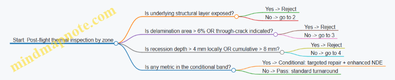
Practical tips that keep criteria usable
- Define zones. A single global threshold is rarely fair. Hot spots deserve stricter criteria.
- Tie each criterion to a method. If you can’t measure it reliably, don’t make it a primary acceptance gate.
- Use consistent grading scales. For oxidation and coating loss, a shared grading rubric prevents “same damage, different inspector” outcomes.
- Document the decision logic. Acceptance criteria should read like an engineering checklist, not a legal document.
Well-defined acceptance criteria reduce ambiguity after flight, where time and access are limited. When thresholds are anchored to performance margins and measurement reality, reuse becomes a controlled engineering process rather than a debate held in the inspection bay.
7. Recovery Operations, Turnaround, and Ground Processing
7.1 Build a Turnaround Plan With Example Scheduling and Resource Allocation
A reusable launch system is only “reusable” if you can reliably return it to flight readiness. The turnaround plan is the bridge between post-flight reality (inspection findings, transport delays, parts availability) and the next launch window. A good plan is specific enough to execute, flexible enough to absorb normal variation, and structured so you can see where time and risk actually go.
Start with a turnaround objective and a flight-readiness definition
Before scheduling tasks, define what “ready” means for each reusable element (stage, engine set, avionics, thermal protection, landing hardware). Use a checklist-style readiness definition that ties directly to acceptance criteria: what must be inspected, what must be repaired, what must be tested, and what must be documented.
A practical approach is to split readiness into three layers:
- Physical readiness: hardware condition meets inspection/repair criteria.
- Functional readiness: required tests and calibrations complete.
- Configuration readiness: correct parts, software versions, and hardware serials installed.
This prevents a common scheduling trap: finishing inspections but discovering late that the configuration baseline or calibration state is not flight-acceptable.
Build a task network, not a list
Turnaround work has dependencies. For example, you cannot reassemble a tank section until you complete NDE, repair, and surface preparation. You also cannot run certain functional tests until you install the correct harness routing and verify connector torque and continuity.
Represent the turnaround as a task network with clear inputs/outputs:
- Inputs: flight data package, telemetry-derived health flags, last-known configuration, spares kit.
- Outputs: inspection reports, repair traveler sign-offs, test results, configuration record.
This makes scheduling more honest because it exposes “waiting on” states rather than hiding them inside optimistic durations.
Mind map: turnaround plan structure
Example scheduling: a 21-day turnaround with explicit gates
Below is an example schedule for a reusable first stage element. Durations are illustrative but structured to show where time typically accumulates. The key is the presence of gates—points where you stop and verify readiness before proceeding.
Assume:
- Vehicle lands and is recovered within 1 day.
- Inspection scope depends on telemetry health flags.
- Some repairs are “standard” (known wear items), while others are “conditional” (triggered by NDE outcomes).
Example day-by-day outline
- Day 0–1: Recovery, secure vehicle, environmental stabilization, initial safety checks.
- Day 1–2: Telemetry review and triage; generate inspection scope and test plan updates.
- Day 2–5: Disassembly to inspection access points; remove thermal protection sections where required.
- Day 5–9: NDE campaign; produce preliminary findings and repair recommendations.
- Day 9–11: Repair decision gate (approve standard repairs vs. escalate to deeper inspection).
- Day 11–15: Repair and rework; surface prep and re-coating; replace serialized parts if needed.
- Day 15–17: Reassembly; harness verification; torque/fit checks; install thermal protection.
- Day 17–19: Functional checkout (power-on checks, sensor calibration, control system verification).
- Day 19–20: System-level verification tests and final configuration audit.
- Day 20–21: Readiness gate sign-off; freeze configuration and release for launch processing.
Add buffers where they matter
Instead of adding a generic “buffer day,” place buffers at dependency chokepoints:
- NDE-to-repair buffer: time for report generation and repair planning.
- Repair-to-integration buffer: time for parts arrival and rework re-planning.
- Checkout-to-acceptance buffer: time for test anomalies and retest.
A simple way to allocate buffers is to reserve:
- 10–20% of the inspection and repair durations as contingency,
- a smaller buffer for integration if tooling and labor are stable.
Resource allocation: match labor to work states
Turnaround labor is not constant. It spikes during disassembly, NDE, and reassembly, then drops during waiting periods for reports, parts, or test scheduling.
A useful allocation method is to define work states and assign roles to each state:
- Safety and recovery state: operations crew, safety officer, range/landing support.
- Triage state: systems engineer, propulsion/structures specialist, QA.
- Inspection state: NDE technicians, structures engineers, documentation control.
- Repair state: repair technicians, materials/finish specialists, QA sign-off.
- Integration state: assembly team, avionics integration, configuration management.
- Test state: test engineers, software/controls support, QA.
Example staffing plan (per shift)
- NDE days: increase NDE technicians and QA inspectors; reduce assembly staffing.
- Repair days: ensure materials/finish specialists are available before reassembly starts.
- Checkout days: keep configuration management and test engineers present to avoid late configuration corrections.
This prevents a common failure mode: the schedule looks fine until the day you discover the QA inspector is booked elsewhere, turning a short task into a multi-day wait.
Critical path identification with a simple dependency view
Use a dependency diagram to identify what actually controls the end date. The critical path is the longest chain of dependent tasks; everything else can slip without changing the final readiness date.
    flowchart TD
  A[Recovery & Safety Checks] --> B[Telemetry Triage]
  B --> C[Disassembly to Inspection Access]
  C --> D[NDE Campaign]
  D --> E[Repair Decision Gate]
  E --> F[Repair & Rework]
  F --> G[Reassembly & Thermal Protection Install]
  G --> H[Functional Checkout]
  H --> I[System Verification & Config Audit]
  I --> J[Readiness Gate Sign-off]
In this example, any delay in NDE, Repair Decision Gate, or Repair & Rework directly pushes the readiness gate.
Make scope changes schedulable, not disruptive
Telemetry triage often changes inspection scope. The plan should include a rule set for how scope changes are handled:
- If a fault flag is within known bounds, apply a standard inspection subset.
- If NDE finds indications beyond thresholds, trigger an escalation path with pre-approved labor and tooling.
The scheduling benefit is that escalation does not start from zero; it starts from a prepared branch.
Example: inspection scope branching with time impact
Inspection Scope Branching (Example)

1) Telemetry health flags: GREEN
- Inspect: standard set
- Expected NDE duration: 4 days
- Repair probability: low

2) Telemetry health flags: YELLOW
- Inspect: standard set + targeted areas
- Expected NDE duration: 5–6 days
- Repair probability: medium

3) Telemetry health flags: RED
- Inspect: full set + deeper NDE
- Expected NDE duration: 7–9 days
- Repair probability: high
- Escalation gate required before reassembly
This keeps the plan executable because the team knows what changes when the color changes.
Turnaround plan outputs you should insist on
A turnaround plan is not complete until it produces artifacts that enable execution:
- A dated schedule with gates and dependency notes.
- A resource plan by role and work state.
- A scope branching rule set tied to telemetry health flags.
- A configuration freeze and documentation sign-off sequence.
When these outputs exist, the turnaround becomes measurable. You can track whether delays are due to inspection findings, parts logistics, test anomalies, or QA sign-off timing—and then fix the real bottleneck rather than rewriting the whole plan.
7.2 Recovery Operations Planning for Landing, Retrieval, and Transport
Recovery operations planning turns a landing event into a repeatable engineering process. The goal is simple: get the vehicle from “on the ground” to “ready for the next flight” with known condition, known configuration, and known schedule. The tricky part is that landing is only the start of the work; the rest is logistics, inspection, and controlled handling.
Recovery operations workflow (end-to-end)
A practical workflow is easiest to manage when it is written as a sequence of states. Each state has entry criteria, exit criteria, and responsible roles.
- Landing and safing: Confirm touchdown, establish safe power state, and secure moving parts. Example: if hydraulic actuators are present, verify pressure bleed-down before any personnel approach.
- Initial survey: Capture external condition quickly while the vehicle is still in a stable environment. Example: photograph and log any soot patterns, sealant residue, or impact marks before washing.
- Hazard control: Manage residual propellants, pressurized lines, and thermal soak. Example: define a “no-touch window” based on measured tank temperatures and valve status.
- Stabilization and access: Position lifting points, deploy covers, and create safe access paths. Example: use alignment pins or guide rails so technicians don’t improvise with ladders near fragile surfaces.
- Inspection and NDE: Perform required inspections based on flight data and observed conditions. Example: if guidance indicates a hard landing, prioritize structural NDE at known load paths.
- Repair or defer: Decide whether hardware is repaired, reworked, or deferred with documented limits. Example: replace a damaged fastener set rather than “tighten and hope” when torque scatter is expected.
- Cleaning and refurbishment: Remove residues and prepare surfaces for reassembly. Example: use cleaning agents compatible with coatings and thermal protection materials.
- Reassembly and functional checks: Install components, verify torque, verify wiring continuity, and run local checks. Example: perform actuator stroke checks with the same command sequence used during integration.
- Transport readiness: Lock down configuration, install protective covers, and verify center-of-gravity constraints for the transport mode.
- Transport and receiving: Move to the next facility, then repeat a receiving inspection to confirm no damage occurred during transport.
Landing site planning: what to decide before the first landing
Recovery planning starts with constraints. You can’t “schedule around” a missing crane capacity or a blocked access road.
Key decisions to document
- Landing site geometry: Define approach paths, safe zones, and where retrieval equipment can operate without interfering with hazards.
- Environmental limits: Specify wind, precipitation, and visibility thresholds for safe operations. Example: if winds exceed a set value, delay lifting operations even if the vehicle is stable.
- Ground conditions: Confirm bearing capacity and traction for transport vehicles. Example: after heavy rain, treat soft ground as a hard stop for heavy lifts.
- Communications and control: Assign a single recovery operations lead with authority to pause work when measurements disagree with expectations.
Retrieval planning: equipment, roles, and timing
Retrieval is where many schedules slip, because it depends on both hardware readiness and human readiness.
Retrieval equipment checklist (example)
- Lifting system sized for the vehicle’s mass and lift points
- Tie-down hardware and load-rated straps
- Tooling for actuator lockout and cover installation
- Portable power and data interfaces for post-landing checkout
- NDE kits for the specific inspection set
Role clarity
- Recovery operations lead: controls go/no-go decisions
- Safety officer: owns hazard controls and permits
- Inspection lead: owns inspection plan execution and sign-off
- Transport coordinator: owns packaging, securing, and route readiness
Timing discipline Create a timeline that includes “measurement gates.” Example: if thermal soak affects inspection outcomes, schedule NDE after temperatures fall below a threshold, not immediately after touchdown.
Transport planning: securing configuration and preventing damage
Transport is not just movement; it is a controlled mechanical event. Planning should treat transport loads as part of the vehicle’s life.
Transport modes and their implications
- Road transport: focus on vibration, tie-down integrity, and suspension behavior. Example: use accelerometer-based checks during a test run to confirm the vehicle doesn’t experience unexpected resonant vibration.
- Crane or hoist transfer: focus on lift dynamics and sling geometry. Example: verify sling angles so the load path matches the lift analysis.
- Containerized transport: focus on interface protection and moisture control. Example: include desiccant where condensation could affect electronics.
Securing and protection practices
- Install protective covers for exposed surfaces and sensors.
- Lock moving parts to prevent relative motion.
- Apply configuration locks so the vehicle arrives at the next facility in the same state it left.
Mind map: recovery operations planning
Concrete example: planning around a “hard landing” indication
Assume flight data indicates a higher-than-nominal landing deceleration and a slightly off-nominal attitude at touchdown.
How that changes recovery planning
- Initial survey: add targeted photo angles for structural interfaces and landing gear attachment points.
- Hazard control: extend the no-touch window if thermal or mechanical loads suggest delayed settling.
- Inspection: prioritize NDE at load paths consistent with the deceleration event. Example: schedule eddy current or ultrasonic checks on fastener rows and adjacent panels.
- Repair decision: if damage is found, define whether the repair is “replace and requalify” or “repair within allowable limits.” The decision should be based on documented acceptance criteria, not technician judgment.
- Transport readiness: ensure any repaired areas are protected from transport vibration and that covers are installed before moving.
The key is that the plan is not generic; it is parameterized by flight data and observed condition.
Concrete example: transport checklist that prevents configuration drift
A common failure mode is arriving at the next facility with a vehicle that is “almost” ready, but missing a cover, a lock, or a documented setting.
A transport checklist should include:
- Configuration locks installed (with part numbers)
- Protective covers installed (with photos)
- Electrical connectors capped or secured
- Control surfaces or actuators locked in the intended position
- Center-of-gravity verification for the chosen transport mode
- Tie-down verification with torque/strap tension records
If you treat this as a checklist with evidence, you reduce rework and avoid inspection surprises.
Documentation and traceability: what must be captured
Recovery operations produce records that connect the landing event to the next flight’s safety case.
Minimum useful outputs:
- As-found log: condition, photos, and any immediate anomalies
- Inspection and NDE records: methods, locations, results, and acceptance decisions
- Repair/defer decisions: what was done, what was not done, and the limits for deferred work
- Configuration state: what is installed, what is removed, and what is locked for transport
- Transport receiving confirmation: a short as-received check to confirm no new issues were introduced
When these outputs are consistent, recovery becomes a controlled process rather than a series of good intentions.
Practical best practices that keep the schedule real
- Write go/no-go criteria in measurable terms (temperature thresholds, wind limits, inspection acceptance). “Looks safe” is not a criterion.
- Plan for the inspection bottleneck by reserving NDE capacity and staffing before retrieval day.
- Separate “vehicle ready” from “team ready” so delays don’t cause rushed work.
- Use evidence-based handoffs between safing, inspection, and transport so each team starts with the same facts.
Recovery operations planning is where engineering meets the real world: ground conditions, human schedules, and physical handling. Done well, it turns a landing into a repeatable system behavior—one that you can inspect, verify, and trust.
7.3 Establish Post-Flight Checkout Procedures With Example Health Check Lists
A reusable launch system only earns its keep if you can answer one question after every flight: “What is safe to reuse, and what needs attention?” Post-flight checkout is the disciplined way to get that answer. It turns raw telemetry, inspection results, and maintenance actions into a clear go/no-go decision with traceable evidence.
Post-flight checkout goals (what “done” means)
- Confirm vehicle state: Verify that measured performance and structural/thermal exposure stayed within the expected envelope.
- Identify life-limiting impacts: Detect whether any component experienced conditions that reduce remaining life (cycles, temperatures, loads, contamination).
- Check functional readiness: Ensure avionics, actuators, valves, sensors, and software configurations are consistent with the next mission.
- Document disposition: Record what was inspected, what was found, what was repaired, and what was cleared.
A practical rule: every checkout item should map to a specific decision. If an item doesn’t change a decision, it probably doesn’t belong.
Mind map: post-flight checkout flow
Checkout philosophy: thresholds, not vibes
Use explicit thresholds for “inspect,” “repair,” and “replace.” For example, a sensor channel might be allowed to drift within a tolerance band; beyond that, you inspect the mounting, wiring, and calibration history before you decide whether the component is reusable.
When thresholds are missing, teams often end up with inconsistent decisions across shifts. A good checkout list prevents that by making the decision logic visible.
Example health check list: reusable first-stage (post-flight)
Below is a concrete checklist structure you can adapt. Each item includes the kind of evidence you should capture and the typical disposition.
A. Flight data review (before opening anything)
-
A1. Mission timeline sanity check
- Evidence: event log vs. expected sequence (stage separation, throttle commands, guidance modes).
- Disposition: go if sequence matches; otherwise open anomaly ticket and hold checkout until root cause is understood.
-
A2. Propulsion performance envelope check
- Evidence: chamber pressure, mixture ratio estimate, thrust profile, valve command tracking.
- Disposition: inspect if any channel deviated beyond set bounds; repair if deviation correlates with a hardware fault indicator.
-
A3. GN&C and attitude control health
- Evidence: IMU bias trends, reaction control usage, control loop stability metrics.
- Disposition: inspect if control authority saturation occurred repeatedly or if sensor residuals exceeded tolerance.
-
A4. Thermal exposure summary
- Evidence: peak temperatures at TPS-adjacent locations, engine bay thermal soak indicators.
- Disposition: inspect TPS and adjacent structures if any peak exceeded the “no inspection required” limit.
B. Safety and contamination checks (while the vehicle is still in a known state)
-
B1. Residual propellant and line integrity
- Evidence: leak check results, pressure decay tests (as applicable), line purge verification.
- Disposition: no-go if any leak rate exceeds threshold; otherwise proceed.
-
B2. Electrical insulation and grounding verification
- Evidence: insulation resistance measurements, connector seating verification.
- Disposition: repair if insulation resistance is out of band; replace suspect harness segments if repeated failures occur.
-
B3. Actuator movement and backlash check
- Evidence: actuator position vs. command response, mechanical play measurement.
- Disposition: inspect if response lag or backlash exceeds limit; repair if friction indicators suggest binding.
C. Engine and propulsion hardware checks (life and wear indicators)
-
C1. Engine borescope inspection
- Evidence: combustion chamber and nozzle wear pattern photos with location tags.
- Disposition: inspect deeper if erosion pattern suggests abnormal mixture or cooling issues; repair/replace if wear exceeds acceptance.
-
C2. Valve and turbomachinery health indicators
- Evidence: valve actuation history, differential pressure trends, vibration metrics.
- Disposition: replace if wear indicators correlate with increased actuation time or abnormal vibration signatures.
-
C3. Seal and gasket condition
- Evidence: seal inspection, torque mark verification, gasket deformation checks.
- Disposition: replace seals if deformation or extrusion is observed; otherwise document “as found” and proceed.
D. Structural and interface checks (damage tolerance meets reality)
-
D1. Fastener and joint inspection
- Evidence: torque stripe verification, visual inspection, NDE on critical joints.
- Disposition: repair if cracks, fretting, or abnormal corrosion is found.
-
D2. Landing/impact load evidence review
- Evidence: accelerometer-derived load metrics, landing gear contact indicators.
- Disposition: inspect adjacent structure if loads exceed the “no additional NDE” threshold.
-
D3. Coating and corrosion check
- Evidence: coating blistering, coating loss areas, corrosion mapping.
- Disposition: repair coating where damage affects protection; escalate if corrosion penetrates beyond allowed depth.
E. Thermal protection system (TPS) checks (repeatability and repair closure)
-
E1. TPS visual inspection and damage mapping
- Evidence: high-resolution photos, damage classification (chips, cracks, delamination signs).
- Disposition: repair if damage exceeds size/count thresholds; otherwise document “no repair required.”
-
E2. Repair verification
- Evidence: repair material batch/lot, cure/processing records, post-repair inspection.
- Disposition: no-go if cure records are incomplete or if inspection shows poor adhesion.
-
E3. Thermal model correlation check (lightweight)
- Evidence: compare measured temps to predicted values at key sensors.
- Disposition: inspect if correlation error exceeds tolerance band, especially near TPS interfaces.
F. Avionics, software, and calibration checks
-
F1. Software build and parameter verification
- Evidence: software version hash, parameter set comparison to baseline.
- Disposition: no-go if mismatch exists; reprogram and re-verify.
-
F2. Fault log review
- Evidence: fault codes since last checkout, cleared vs. persistent faults.
- Disposition: repair if any persistent fault indicates degraded sensor/actuator behavior.
-
F3. Sensor calibration status
- Evidence: calibration dates, last known bias values, in-flight residuals.
- Disposition: recalibrate if drift exceeds tolerance or if calibration is overdue.
G. Evidence pack and readiness decision
-
G1. Discrepancy resolution
- Evidence: list of discrepancies, disposition, and sign-offs.
- Disposition: no-go until every discrepancy has a documented closure.
-
G2. Component life accounting
- Evidence: updated cycle counts, hot-fire counts, maintenance actions tied to serial numbers.
- Disposition: no-go if life counters are inconsistent or missing.
-
G3. Final readiness review
- Evidence: checklist completion status, photos/NDE reports attached, configuration verified.
- Disposition: go/no-go issued by designated authority.
Example “health check list” template (copyable structure)
Health Check Item: ________
System/Area: ________
Trigger: (post-flight / anomaly / schedule)
Evidence Required: ________
Method/Tool: ________
Acceptance Criteria:
- Inspect if: ________
- Repair if: ________
- Replace if: ________
Results (As Found): ________
Disposition: (Go / Inspect / Repair / Replace)
Actions Taken: ________
Reference Docs/Photos: ________
Sign-off: ________
Practical tips that prevent checkout from becoming paperwork
- Use “as found” photos before any cleaning or repair. It’s easier to interpret damage patterns when you still have the original state.
- Tie every action to a threshold. If you repaired something “just in case,” you’ll struggle to justify the decision later.
- Separate “data review” from “hardware work.” Data review can hold the line early, while hardware work should only start when you’ve identified what matters.
- Keep the list short enough to finish. A checklist that can’t be completed reliably will be skipped, which defeats the purpose.
A strong post-flight checkout procedure is less about exhaustive coverage and more about consistent decision-making. When the evidence pack is complete and every item has a clear disposition path, reuse becomes an engineering activity you can audit—not a guess you hope is right.
7.4 Manage Consumables and Reuseable Hardware Tracking With Example Traceability Practices
Reusable launch systems don’t fail only in the obvious places like engines and guidance. They also fail in the boring places: a missing seal, a reused fastener that should have been replaced, a tank that still has residue, or a consumable that was “probably” used last time. The fix is not hope; it’s traceability with operational discipline.
This section focuses on two intertwined tasks:
- managing consumables (items consumed or degraded by flight/processing), and
- tracking reusable hardware (items that survive multiple flights but still accumulate wear, inspection results, and configuration changes).
What to track (and what not to track)
Start by separating items into three categories.
- Consumables: items that are consumed, replaced, or whose condition changes in a way that makes reuse unacceptable (e.g., gaskets, filters, certain valves, thermal blankets that must be inspected and often replaced).
- Reusable hardware: items that are intended to fly again, but require life tracking and inspection history (e.g., engines, avionics boxes, landing legs, reusable TPS panels).
- Process-only items: items used during processing but not part of the flight configuration (e.g., temporary rigging hardware). These usually need batch control, not flight traceability.
A practical rule: if an item’s state can affect flight safety, performance, or compliance, it needs a traceable identity tied to a specific flight and processing cycle.
Traceability model: identity, state, and linkage
A traceability record should answer three questions:
- Identity: What is it? (serial number, part number, revision)
- State: What condition is it in? (inspection results, life counters, configuration)
- Linkage: Where did it go and when? (which stage, which flight, which processing event)
If you only track identity, you can still reuse the wrong configuration. If you only track state, you can still lose the chain of custody. If you only track linkage, you can’t prove what condition existed.
Mind map: consumables and reusable hardware tracking
Example traceability practice 1: “Kitting with proof,” not just a checklist
During processing, teams often use a kitting list: “install these items.” The improvement is to make the list require proof of identity.
Practice: generate a kit for a specific stage and processing event, then require each item to be scanned (or otherwise uniquely recorded) at the moment it is staged for installation.
Example:
- A reusable stage uses a set of O-ring seals in a specific manifold location.
- The kit record includes: part number, revision, and acceptable serial range (or batch ID).
- When the technician opens the kit, they log the exact serial/batch IDs.
Why this matters: if a seal is swapped due to a supply issue, the system can flag it immediately because the kit is tied to the expected configuration.
Minimal record fields for each consumable item:
ItemID(serial or batch)PartNumber+RevisionKitID+StageLocationInstallTimestamp(orStagedTimestampif install is later)Operator(or team ID)
Example traceability practice 2: Life counters tied to the physical item
Reusable hardware needs life tracking that follows the item, not the vehicle.
Practice: maintain life counters per serial number and update them only when an event that changes life occurs.
Example:
- An engine turbopump has a life limit expressed as equivalent hot-fire hours.
- After each flight, the post-flight checkout computes equivalent hours from recorded engine parameters.
- The life counter update is written to the engine’s serial record.
Key control: the update is linked to the flight ID and the data source used for the computation.
Minimal record fields for reusable hardware:
HardwareSerialLifeCounterType(e.g., hot-fire equivalent hours)LifeCounterValueLastUpdateFlightIDComputationMethodID(or data set ID)InspectionDueDateorInspectionDueThreshold
This prevents the classic failure mode: “the counter exists, but nobody knows which flight it came from.”
Example traceability practice 3: Configuration snapshots at readiness
Configuration drift is subtle. A fastener type changes. A sensor is replaced with a different revision. Software is updated on one box but not another. If you only track “what we intended,” you’ll eventually install “what we actually did.”
Practice: create a configuration snapshot at the point of readiness-to-fly.
Example snapshot contents for a stage avionics bay:
- Each box serial number
- Hardware revision of connectors and harness assemblies
- Firmware/software versions per box
- Any installed options (e.g., specific landing sensor set)
- The list of consumables that are installed and their batch IDs (where relevant)
Why it’s operationally useful: when a post-flight anomaly occurs, you can compare the snapshot to the expected configuration and quickly identify what changed.
Mind map: linkage and gating
Consumables: tracking patterns that work in practice
Consumables vary, but the tracking approach can be consistent.
- Batch-controlled consumables (e.g., filters, seal kits)
- Track batch ID and expiration/lot acceptance.
- Record install location.
- Condition-controlled consumables (e.g., items that must be inspected before reuse)
- Track inspection method and result.
- Record whether the item was replaced or reinstalled.
- Consumables with “use count”
- Some items are not consumed in a single flight but degrade with repeated processing cycles.
- Track cycles, not just “installed once.”
Reusable hardware: tracking patterns that prevent “silent drift”
- Serial-first tracking
- Every reusable item has a unique ID.
- Life counters and inspection history attach to that ID.
- Location-aware installation records
- A serial number is not enough; you also need where it was installed.
- This matters when a component can be swapped between bays or stages.
- Inspection gating tied to due thresholds
- If an inspection is due, the system should block reuse until the inspection result is recorded.
Example: a compact traceability record schema
Below is a simple structure you can map to a database or a paper traveler. The goal is not the exact format; it’s the completeness.
ConsumableRecord
- ItemID (serial or batch)
- PartNumber + Revision
- StageLocation
- KitID
- InstallTimestamp
- Operator/Team
- InstallEvidenceRef

ReusableHardwareRecord
- HardwareSerial
- PartNumber + Revision
- StageLocation
- LifeCounterType
- LifeCounterValue
- LastUpdateFlightID
- InspectionDueThreshold
- LastInspectionResultRef
- ConfigurationSnapshotRef
Operational example: end-to-end traceability for one stage
Imagine a stage that flies, returns, and is processed for the next mission.
- Post-flight checkout: the team records inspection results for reusable hardware serials, including methods used (e.g., visual, NDI) and pass/fail.
- Consumable kitting: the next kit is generated for the stage processing event. Each consumable item is scanned into the kit with batch IDs.
- Install logging: when items are installed, the traveler logs the exact ItemID and the stage location.
- Life counter update: engine life counters are updated using the flight’s recorded parameters, linked to the flight ID.
- Readiness snapshot: before mating and final closeout, the stage configuration snapshot is created, listing all reusable hardware serials, their revisions, and the installed consumables’ batch IDs.
If an anomaly later points to a specific subsystem, you can trace backward: which serials were installed, which consumables were used, and what inspection evidence existed at readiness.
Practical checklist for traceability quality
- Every reusable item has a serial-based record with life and inspection history.
- Every consumable that affects safety or compliance has a batch/serial-based record tied to install location.
- Every install/remove action is linked to a processing event.
- Every readiness snapshot references the exact set of installed items.
- No life counter update or reuse decision is recorded without an event ID and evidence reference.
When these controls are in place, reusability becomes an engineering discipline rather than a paperwork exercise. You still do the hard work—design, test, inspect—but you can prove what you did and why, with traceability that holds up under scrutiny.
7.5 Reduce Turnaround Risk Using Example Bottleneck Analysis and Mitigation
Turnaround risk is usually not one big failure mode. It’s a chain of small delays: an inspection takes longer than planned, a part is missing, a test stand is booked, or a repair decision waits on one piece of data. The goal is to reduce the probability that any single link in that chain becomes the bottleneck.
Step 1: Build a turnaround flow with time and dependency tags
Start with a flight-to-ready workflow that includes both physical work and decision work. For each step, record:
- Duration distribution (not just an average): e.g., 6–10 hours with a typical 8.
- Inputs required: hardware access, data products, consumables, tooling.
- Outputs produced: inspection report, test result, release-to-assemble.
- Dependencies: who signs off, which lab runs the NDE, which QA gate must clear.
A simple example flow for a reusable stage might look like:
- Stage offload and safing
- Visual inspection and leak check
- NDE on critical welds and tank regions
- Engine bay inspection and borescope
- Thermal protection inspection (if applicable)
- Repair decision and parts kitting
- Repair execution
- Reassembly and torque verification
- Integrated checkout (avionics, pneumatics, hydraulics)
- Final acceptance and release
The key is to tag steps that are decision-gated (repair decision, release-to-assemble) and resource-gated (NDE lab slot, test stand time). Those are the usual bottleneck sources.
Step 2: Identify bottlenecks with a “critical path” mindset
A bottleneck is a step that either:
- consumes the most time, or
- has the most dependencies, or
- has the highest variability, or
- blocks multiple downstream tasks.
You can do this without heavy math by using a “variability-weighted critical path” approach:
- Mark each step as A (high variability), B (high dependency count), or C (long duration).
- The bottleneck candidates are steps with the highest combination of A/B/C.
Here’s a mind map that captures the typical bottleneck categories for reusable hardware turnaround.
Turnaround Bottleneck Mind Map
Step 3: Use an example bottleneck analysis table
Consider a reusable stage where the plan targets 10 days from landing to ready. The schedule is mostly fine until a single step starts slipping.
Example: NDE and repair decision.
| Step | Planned duration | Variability | Dependency count | Bottleneck risk driver | Typical mitigation lever |
|---|---|---|---|---|---|
| NDE setup + access | 6 h | Medium | 3 | Waiting for access window | Pre-stage access checklist; staged tooling readiness |
| NDE execution | 18 h | High | 2 | Lab slot and rework cycles | Reserve lab slot; define rework triggers |
| NDE report review | 8 h | Medium | 4 | QA/engineering review queue | Pre-brief review criteria; assign reviewers |
| Repair decision | 4 h | High | 5 | Missing data or unclear acceptance | Decision rubric; “if data missing, do X” rule |
| Parts kitting | 12 h | Medium | 3 | Serialization and lead time | Kitting by serial; dual-source consumables |
In this example, the repair decision step is the real bottleneck even though it’s short. It has the highest dependency count and high variability because it depends on whether the NDE report includes the specific measurements needed for acceptance.
Step 4: Mitigate bottlenecks with targeted controls
Mitigation should be specific to the bottleneck driver. Below are practical controls that map cleanly to the table.
- Pre-commit decision criteria (reduce decision variability) Create a short “repair decision rubric” that states what triggers repair, what triggers acceptance, and what triggers additional data collection. The rubric should reference the exact inspection outputs you expect from NDE.
Example rubric logic:
- If measured crack length \( L \le L_{acc} \) and growth rate estimate is below threshold, accept with monitoring.
- If \( L_{acc} < L \le L_{rep} \), perform localized repair.
- If required measurement is missing (e.g., no through-thickness estimate), run a defined follow-up NDE method rather than waiting for ad hoc engineering.
This turns “waiting for clarity” into “run the next step.”
- Reserve capacity where variability is highest (reduce resource gating) If the NDE lab is the constraint, reserve the slot based on the worst-case inspection plan, not the average. Then allow a controlled release if results are clean.
Example practice:
- Book the NDE slot for the full inspection set.
- If early screening indicates no action required, cancel the remaining sub-tests and free the slot for the next vehicle.
That keeps the schedule from collapsing when you need the time.
- Design for “data completeness” at the start (reduce missing inputs) Turnaround often stalls because the team is missing one data product: a sensor calibration record, a flight log segment, or a health report summary.
Example control:
- Define a “minimum data package” required to start repair decision review.
- If the package is incomplete, the workflow routes to a data recovery step with a time limit.
- Use kitting rules that match traceability reality (reduce logistics delays) Parts delays are rarely about the parts themselves; they’re about the paperwork and matching.
Example practice:
- Kit by serial number and configuration state.
- Include a “no-go” check: if the reused part’s configuration doesn’t match the expected interface revision, stop and resolve before assembly.
- Add buffer where it matters, not everywhere (reduce schedule risk without inflating cost) Buffers should be placed at bottleneck steps, not sprinkled randomly. A useful approach is to add a buffer equal to the difference between the 90th percentile and the planned duration for the bottleneck step.
If NDE report review is planned at 8 hours but typically takes 12 hours at the 90th percentile, add a 4-hour buffer there. Don’t add 4 hours to every step.
Step 5: Track bottleneck performance with simple leading indicators
After each turnaround, update your bottleneck model using leading indicators that predict schedule slip early.
Example leading indicators:
- Inspection rework rate: fraction of NDE areas requiring repeat scans.
- Decision cycle time: time from “NDE report ready” to “repair decision issued.”
- Data package completeness: percent of minimum data package items available at review start.
- Kitting readiness: percent of parts ready before the first assembly attempt.
A mind map helps keep these indicators tied to the bottleneck categories.
Bottleneck Mitigation Mind Map
Worked mini-example: preventing a one-week slip
Suppose the team’s plan assumed NDE report review would finish in 8 hours. In the last turnaround, it took 14 hours because reviewers waited for one missing measurement.
Mitigation applied:
- The repair decision rubric now specifies that if the through-thickness estimate is missing, the workflow triggers a follow-up NDE method within 6 hours.
- The minimum data package gate blocks repair decision review until the through-thickness estimate is present or the follow-up is scheduled.
Result in the next turnaround:
- Even when the first NDE run misses the measurement, the follow-up is executed immediately.
- The decision cycle time becomes bounded by the follow-up window rather than by engineering availability.
The turnaround doesn’t become “perfect.” It becomes predictable, which is what reduces risk.
Practical checklist for the bottleneck owner
- Have you identified the top 3 steps by variability and dependency count?
- Do you have a decision rubric that prevents “waiting for clarity”?
- Are capacity reservations aligned to the inspection plan you might need?
- Is there a minimum data package gate with a time-limited recovery path?
- Are kitting and configuration checks preventing late assembly stops?
- Are buffers placed at bottleneck steps using percentile differences?
When these controls are in place, turnaround risk shifts from surprise delays to managed exceptions. That’s the engineering version of making the schedule behave: fewer unknowns, tighter gates, and clear next actions when reality doesn’t match the plan.
8. Verification, Validation, and Reuse-Oriented Testing
8.1 Create a Reuse-Focused Verification Plan From Requirements to Tests
A reuse-focused verification plan answers one question early: what evidence will convince us the reused hardware will work again, not just once? The trick is to start from requirements that explicitly mention reuse, then trace them to testable claims. If a requirement can’t be tied to a measurable outcome, it’s usually a sign the verification plan will become a list of activities instead of a logic chain.
Step 1: Start with reuse-aware requirements (and make them testable)
Begin with the top-level mission and system requirements, then add reuse-specific qualifiers. Examples:
- Reusable stage performance requirement: “The stage shall deliver nominal ascent performance for up to N flights with no more than X% thrust shortfall at ignition.”
- Reusable landing requirement: “The stage shall land within Y meters of target with probability P given post-flight inspection acceptance criteria.”
- Reusable engine life requirement: “The engine shall complete N cycles with hot-fire time per cycle within tolerance, and shall meet thrust margin and vibration limits after each cycle.”
A practical check: for each requirement, write a one-sentence “verification claim” that states what must be observed. For instance, for the engine life requirement, the claim might be: “After N cycles, the engine meets thrust and vibration limits under representative operating conditions.” That claim becomes the anchor for test selection.
Step 2: Build a traceable verification logic chain
Use a simple structure: Requirement → Verification Objective → Evidence Type → Test/Analysis Method → Acceptance Criteria.
- Evidence type can be test data, analysis results, inspection outcomes, or similarity arguments.
- Test/analysis method should match the claim. If the claim is about post-flight condition, a pre-flight test alone won’t cover it.
- Acceptance criteria must be numeric or operationally defined. “Meets requirements” is not an acceptance criterion; it’s a placeholder.
Here’s a compact example for a reusable avionics box:
- Requirement: “Avionics shall maintain navigation accuracy after reuse.”
- Verification objective: quantify navigation error growth after refurbishment.
- Evidence type: test data.
- Method: end-to-end navigation test with representative sensor inputs after refurbishment.
- Acceptance criteria: navigation solution error ≤ threshold over specified time window.
Step 3: Identify reuse-relevant failure modes and map them to tests
Reuse changes the risk profile. A component that works once can fail on the second or third flight due to wear, loosened interfaces, seal degradation, or accumulated thermal/mechanical damage.
A good reuse-focused plan explicitly covers:
- Life-limiting degradation (fatigue, erosion, corrosion, seal wear)
- Post-repair variability (tolerances, reassembly effects, workmanship)
- Environment carryover (residual contamination, trapped moisture, insulation damage)
- Interface integrity (connectors, mounts, fasteners, alignment)
A useful technique is to start from a failure mode list (FMEA or fault tree) and tag each failure mode with a reuse trigger: “worsens with cycles,” “depends on refurbishment,” or “depends on landing loads.” Then you decide whether to verify via test, inspection, or analysis.
Step 4: Choose a test strategy that matches the reuse question
A verification plan typically mixes four categories:
- Qualification tests: prove design adequacy for the intended environment and life.
- Acceptance tests: confirm each reused unit is “ready to fly” after refurbishment.
- Regression tests: ensure changes (software, procedures, repairs) don’t break prior performance.
- Characterization tests: fill gaps where you need data to support inspection thresholds or model updates.
Example: Suppose you have a reusable thermal protection panel.
- Qualification: thermal cycling and impact tests on representative coupons.
- Acceptance: inspection + localized thermal performance test on each panel set.
- Regression: repeat a subset of thermal tests after process changes (adhesive lot, surface prep).
- Characterization: correlate inspection findings (e.g., surface roughness or delamination indicators) to thermal performance.
The plan should state which category covers which claim. If a claim is about “after refurbishment,” then acceptance or characterization must be involved.
Step 5: Define inspection and refurbishment verification as first-class evidence
Reuse isn’t only about hardware surviving; it’s also about the process producing consistent results. Treat inspection and repair steps like verification steps with measurable outputs.
For each critical item, define:
- Inspection method (NDE type, measurement location, resolution)
- Pass/fail criteria (numeric thresholds or clearly defined conditions)
- Rework/repair actions (what happens when borderline)
- Re-verification (what test or inspection confirms the repair worked)
A simple example for a reused structural joint:
- Inspect: ultrasonic thickness and bond integrity at specified zones.
- Criteria: minimum thickness and no disqualifying indications.
- If borderline: rework surface prep and re-bond.
- Re-verify: repeat ultrasonic scan and perform a localized mechanical test on a representative coupon from the same repair batch.
Step 6: Create a test matrix that covers both life and variability
A reuse-focused matrix should cover:
- Cycle count: at least one test point at the expected maximum cycle and one below it.
- Refurbishment state: “as refurbished” units, not only pristine units.
- Operating conditions: representative ranges (temperatures, pressures, loads).
- Uncertainty sources: sensor calibration drift, assembly tolerances, inspection variability.
A practical way to keep it manageable is to define representative test articles and representative refurbishment processes. If you test a perfect unit and then refurbish with a different process, you’ve verified the wrong thing.
Mind map: Requirements to tests for reuse
Example: A small verification plan fragment (engine)
Requirement: “After N reuse cycles, the engine shall meet thrust margin ≥ M and vibration RMS ≤ V during a representative hot-fire profile.”
Verification objective: demonstrate performance retention after refurbishment and accumulated wear.
Evidence type: test data.
Method:
- Build test articles that undergo refurbishment between cycles using the same procedure as operations.
- Run hot-fire profiles at representative chamber pressure and mixture ratio.
- Measure thrust, vibration, and key temperatures.
Acceptance criteria:
- Thrust margin ≥ M for each cycle or at least at the final cycle (state which).
- Vibration RMS ≤ V over defined frequency bands.
- Any parameter outside limits triggers a defined disposition path (repair, re-test, or reject).
Why this is reuse-focused: the test includes refurbishment between cycles, so the evidence covers both wear and process variability.
Step 7: Close the loop with configuration and data handling
A verification plan should specify how evidence becomes a decision. Include:
- Configuration scope: what exact hardware and software versions are tested.
- Data traceability: how test data links to the unit serial number and refurbishment record.
- Decision rules: who approves acceptance, what happens when results are near thresholds.
This prevents a common failure mode: you collect good data, but you can’t prove it applies to the reused unit being prepared for flight.
Step 8: Write the plan so it can be executed
A reuse-focused plan is readable by the people who run tests and inspections. For each verification objective, include:
- purpose (what claim it supports)
- test article definition
- procedure summary
- instrumentation list (high level)
- acceptance criteria
- evidence storage location and naming convention
- linkage to refurbishment steps
If you can’t summarize an objective in a short checklist, it’s likely too vague to be useful.
Summary
A reuse-focused verification plan is a chain of testable claims: reuse-aware requirements become verification objectives, which become evidence types and methods, which become acceptance criteria. The plan stays credible when inspection and refurbishment are treated as verification steps, and when the test matrix covers both life and the variability introduced by reassembly.
8.2 Use Incremental Test Campaigns With Example Hardware Readiness Levels
Incremental test campaigns are how you keep reusability from becoming a “trust me” exercise. The idea is simple: start with what you can learn safely, then add realism in steps—while tracking readiness with explicit hardware readiness levels (HRLs). Each step should answer a specific question, not just generate data.
Why incremental campaigns work for reusable hardware
Reusable launch systems face a recurring problem: the hardware is not only “proven once,” it must survive repeated environments and repeated handling. That means you need evidence for:
- Physical survival (life, damage tolerance, thermal/structural margins)
- Process repeatability (inspection, repair, reassembly, checkout)
- Integration stability (interfaces, software behavior, sensor/actuator health)
Incremental campaigns let you separate these concerns. You can validate a subsystem’s behavior without committing the full stack to a full-duration, full-environment test.
Hardware Readiness Levels (HRLs): a practical example
Below is an example HRL ladder you can adapt. The key is that each level has a clear entry criterion and a clear exit criterion.
Example HRL definitions
- HRL 1 — Component breadboard: Functional demonstration of key mechanisms or algorithms using non-flight hardware.
- Exit evidence: Demonstrates the intended function in a controlled setting.
- HRL 2 — Subsystem engineering unit: Relevant interfaces and representative materials; limited environment exposure.
- Exit evidence: Shows performance within requirements in lab conditions.
- HRL 3 — Subsystem qualification unit: Hardware built to qualification configuration; representative environment tests.
- Exit evidence: Meets acceptance criteria for the defined test envelope.
- HRL 4 — Flight-representative unit (pre-production): Near-flight configuration; includes realistic integration, wiring, and software hooks.
- Exit evidence: Passes end-to-end subsystem tests including fault handling.
- HRL 5 — Flight unit (reusable configuration): Hardware intended for flight use, with traceability to the production/repair process.
- Exit evidence: Passes acceptance tests and is cleared for operational use.
- HRL 6 — Reuse-validated unit: Demonstrates repeat-use behavior through multiple cycles relevant to the mission profile.
- Exit evidence: Meets life and post-cycle inspection thresholds across cycles.
A reusable system typically needs HRL 5 for “first flight,” but HRL 6 for “repeat flights without surprises.”
Mind map: incremental campaign structure
Campaign design: start narrow, then widen
A good incremental campaign has a “learning gradient.” You increase realism only after you can explain what you saw.
Step 1: single-parameter learning (HRL 1 → HRL 2)
Pick one dominant driver for the reusable subsystem. For example, if you’re testing a thermal protection attachment method, the dominant driver might be cycle-to-cycle bond degradation.
Example test objective:
- Demonstrate that the attachment survives repeated thermal excursions without unacceptable loss of bond strength.
Example HRL progression:
- HRL 1: coupons or small panels with representative materials, tested for bond behavior.
- HRL 2: a representative subassembly with realistic mounting geometry and instrumentation.
What you record:
- Temperature histories at multiple depths
- Post-test inspection metrics (crack length, delamination area, surface changes)
- Variability across samples, because reusability amplifies scatter
Decision gate:
- Promote only if the measured degradation trend is bounded and the inspection method can detect it reliably.
Step 2: interface realism (HRL 2 → HRL 3)
Interfaces are where “it worked in the lab” goes to die. For reusable hardware, interfaces include not only mechanical and electrical connections, but also software assumptions and health monitoring logic.
Example test objective:
- Verify that sensor readings and actuator commands remain consistent after representative handling.
Example practice:
- Run a sequence test that includes connector mate/demate cycles, harness routing checks, and fault injection (e.g., stuck sensor, intermittent power).
Decision gate:
- Promote only if fault handling behavior is deterministic and post-test calibration/zeroing procedures are repeatable.
Step 3: environment realism (HRL 3 → HRL 4)
Now you add the environment that matters for survival. For reusable stages, that often means repeated thermal loads, repeated structural loads, and repeated cooldown/heat soak patterns.
Example test objective:
- Demonstrate that the subsystem meets acceptance criteria after representative thermal/structural loading.
Example practice:
- Use a test matrix that varies the most sensitive parameters (e.g., peak temperature, dwell time, load rate) while holding others constant.
Decision gate:
- Promote only if model correlation is adequate for the next step. If you can’t explain the data, you can’t justify the next realism jump.
Step 4: process realism (HRL 4 → HRL 5)
This is the part many teams underweight: reusability is a process, not just a hardware property. Your campaign should include inspection, repair, reassembly, and checkout.
Example test objective:
- Prove that the inspection method and repair procedure restore the subsystem to an acceptable state.
Example practice:
- After an environment test, perform NDE (nondestructive evaluation), apply a defined repair action for representative findings, then reassemble and run a checkout sequence.
Decision gate:
- HRL 5 requires that the “repair-to-acceptance” loop is repeatable across multiple units and multiple cycles.
Step 5: reuse-validated cycles (HRL 5 → HRL 6)
HRL 6 is where you demonstrate repeat-use behavior. The goal is not to test forever; it’s to test enough cycles to support the operational claim with evidence.
Example test objective:
- Demonstrate that life-limiting mechanisms remain within limits across the defined number of reuse cycles.
Example practice:
- Run cycles that mirror operational handling: thermal exposure, mechanical loading, inspection, repair (if applicable), and post-cycle acceptance.
Decision gate:
- Promote only if post-cycle inspection thresholds are met and the failure modes observed are understood and bounded.
Example: a reusable engine component campaign (condensed)
Suppose you’re qualifying a valve assembly that must survive repeated hot-fire exposure.
- HRL 1: Bench test of actuation and sealing using simplified thermal conditions.
- HRL 2: Representative assembly with realistic materials and instrumentation; limited thermal cycling.
- HRL 3: Qualification unit tested across the defined thermal and pressure envelope.
- HRL 4: Flight-representative integration with harness, sensors, and fault injection.
- HRL 5: Flight unit acceptance tests plus process rehearsal (inspection and reassembly).
- HRL 6: Multiple hot-fire cycles with post-cycle NDE and acceptance checks.
The campaign is incremental because each step adds realism in a controlled way, and each promotion has evidence tied to acceptance criteria.
Acceptance criteria and readiness promotion: keep it concrete
To avoid “HRL inflation,” define:
- Quantitative acceptance criteria (e.g., leak rate limits, bond strength thresholds, dimensional tolerances)
- Inspection method capability (can you detect relevant damage reliably?)
- Traceability from test results to requirements
- Clear promotion rules (what must pass, what can be waived, and who decides)
A simple rule of thumb: if a test result can’t change a decision, it probably shouldn’t be in the campaign.
Common pitfalls (and how incremental structure prevents them)
- Skipping process realism: If you only test hardware, you’ll discover repair and inspection surprises late. Step 4 fixes that.
- Overloading one test step: If you try to prove survival, integration, and process all at once, you lose diagnostic clarity. The learning gradient prevents it.
- Vague HRL definitions: If HRLs are just labels, they won’t guide decisions. Explicit entry/exit criteria keep the ladder meaningful.
Incremental test campaigns are essentially risk management with receipts. When HRLs are defined tightly and each step has a specific question, reusability becomes an engineering claim supported by evidence rather than a hope supported by schedules.
8.3 Validate Software and Control Laws With Example Regression and Hardware-in-the-Loop
Reusable launch systems live or die by repeatability. For software and control laws, “repeatable” means the same inputs produce the same outputs within known tolerances, even after code changes, sensor quirks, and hardware wear. The validation approach below focuses on two things: (1) proving the control logic behaves correctly across a defined set of scenarios, and (2) proving that future changes don’t quietly break those behaviors.
What you validate (and what you don’t)
Start by separating control validation into three layers:
- Control-law correctness: guidance, navigation, control, and actuator command logic produce stable, bounded outputs for the modeled plant.
- Interface correctness: sensor scaling, timing, unit conversions, message framing, and mode transitions work exactly as specified.
- Closed-loop behavior under realistic I/O: the controller reacts properly when the hardware-in-the-loop (HIL) injects sensor noise, latency, dropout, and actuator saturation.
A common mistake is to treat “controller passes in simulation” as “controller passes in flight.” Simulation often assumes perfect timing and clean measurements. HIL exists to remove that assumption.
Mind map: regression and HIL validation flow
Regression + HIL validation mind map
Build a regression suite that is actually useful
A regression suite is not a pile of tests; it’s a curated set that catches the most likely breakpoints. For reusable launchers, those breakpoints often cluster around mode logic, actuator limits, and sensor scaling.
1) Choose a deterministic replay strategy Make every regression run reproducible. That means:
- Fix random seeds for any stochastic elements.
- Pin model parameters and configuration files.
- Ensure the same sample rates and scheduling order.
2) Define scenario buckets Instead of “test everything,” define buckets that map to requirements. Example buckets for ascent guidance and control:
- Nominal tracking: reference trajectory tracking with nominal mass and thrust.
- Mass property mismatch: ±X% propellant mass or center-of-mass shift.
- Aero uncertainty: drag coefficient perturbation and wind shear.
- Sensor bias: IMU bias step and accelerometer scale error.
- Actuator saturation: max gimbal or throttle limit reached.
- Mode transitions: guidance mode switch at a specific event time.
Each bucket should include at least one “tight” case (near the boundary) and one “loose” case (comfortably inside limits). The tight case is what prevents regressions from slipping through.
3) Use pass/fail thresholds tied to control requirements Examples of thresholds that are concrete and measurable:
- Tracking error: \(|e(t)| \le e_{max}\) for the duration of the phase.
- Stability proxy: commanded acceleration remains bounded and does not oscillate beyond a specified envelope.
- Saturation behavior: saturation occurs fewer than \(N\) times per second, or recovers within \(T\) seconds after leaving the limit.
- Mode transition: no illegal intermediate mode, and outputs remain within safe bounds during the transition window.
If you don’t have thresholds yet, regression becomes “did it look okay?” which is not validation.
Example regression test vectors (what to store)
Store test vectors as versioned artifacts so you can replay them later. A test vector typically includes:
- Time series for reference commands (or initial conditions that generate them)
- Sensor input streams (or parameters to generate them)
- Fault injection flags (if any)
- Model parameter set identifiers
Here’s a compact example of what a regression case might record.
{
  "caseId": "ASC-GNC-TRACK-COAST-001",
  "phase": "ascent",
  "modelParams": {"massKg": 82000, "cmShiftMm": 120, "cdScale": 1.03},
  "sensor": {"imuBias": [0.02, -0.01, 0.03], "gyroScale": 1.001},
  "timing": {"latencyMs": 8, "jitterMs": 1},
  "faults": {"none": true},
  "assertions": {
    "maxTrackingErrorM": 35,
    "maxCmdAccelMps2": 18,
    "saturationRecoverySec": 2.5
  }
}
HIL validation: prove the controller survives real I/O
HIL validation should focus on the controller’s interaction with hardware-like signals. The key is to test the same scenarios as regression, but with realistic I/O behavior.
1) Validate timing and scheduling assumptions Control loops are sensitive to timing. In HIL, verify:
- The controller receives sensor updates at the expected rate.
- The control computation finishes before the actuator command deadline.
- Latency and jitter match the emulation configuration.
A practical check is to log timestamps at three points: sensor sample time, controller read time, and actuator command output time. Then verify the end-to-end delay stays within the allowed window.
2) Inject actuator saturation and confirm limit handling Actuator saturation is where many control regressions hide. In HIL, explicitly test:
- Saturation onset: does the controller wind up integrators or accumulate error?
- Saturation persistence: does the controller remain stable while commands are clipped?
- Saturation recovery: does it return to linear behavior quickly and smoothly?
A simple metric is “time to exit saturation” and “overshoot after recovery.” If recovery is slow or overshoot grows, the issue often isn’t the plant—it’s the control-law bookkeeping.
3) Test mode transitions with realistic bus behavior Mode transitions are often triggered by events (altitude, velocity, time, or state estimates). In HIL, emulate:
- Message delays or dropped frames (within defined limits)
- Out-of-order events (if your system can tolerate them)
- Mode command contention (two sources requesting different modes)
The acceptance criteria should be explicit: which mode wins, what the controller outputs during the transition, and how quickly it converges.
Example HIL test: closed-loop tracking with fault injection
Consider a controller that tracks a commanded pitch angle and rate during a phase. A HIL test can combine:
- A nominal reference trajectory
- A step bias in gyro measurement
- A brief sensor dropout
- A throttle limit event that forces actuator saturation
Your evaluation should include:
- Tracking error bounds during nominal and fault windows
- Controller output boundedness (no runaway commands)
- Fault containment: after dropout ends, does the controller re-acquire smoothly?
- No illegal mode transitions
To keep this measurable, define assertions like:
- \(e_{pitch}(t)\) stays below a higher bound during the fault window, but returns below the nominal bound within \(T\) seconds.
- Actuator command remains within physical limits at all times.
- After sensor dropout, the controller does not oscillate with growing amplitude.
Automate the evidence: regression reports that engineers trust
A regression run should produce a report that answers three questions quickly:
- Which cases ran, and which were skipped (with reasons)?
- Which assertions passed or failed, and by how much?
- What changed since the baseline (code version, model version, config version)?
A good report includes plots for the failed cases only, plus a table of assertion results. That keeps review time focused.
Regression report checklist
- Case list with versioned case IDs
- Model/config identifiers
- Assertion table (pass/fail + numeric margins)
- Timing summary (latency/jitter stats)
- Saturation summary (count, duration, recovery time)
- Mode transition log (timestamps + final mode)
- Links to raw logs for failed cases
Common failure modes (and how regression/HIL catches them)
- Unit mismatch: scaling errors that simulation might not reveal if the model uses ideal units. HIL catches it because sensor emulation uses the same scaling path as flight.
- Integrator wind-up: saturation causes integrator growth, which later produces overshoot. HIL with saturation events makes this obvious.
- Mode logic edge cases: off-by-one timing around event thresholds. Regression with tight boundary cases catches it before HIL.
- Timing overruns: code changes that increase computation time. HIL timing logs show deadline misses.
Practical workflow: from regression to HIL to sign-off
- Run regression on every code change with deterministic replay.
- If regression passes, run the most sensitive HIL scenarios (mode transitions, saturation, sensor bias/dropout).
- Compare HIL results against the baseline using the same metrics and thresholds.
- Only then approve the build for further integration steps.
This workflow keeps the validation effort proportional: you use fast regression to filter most issues, and you use HIL to confirm the tricky parts where real I/O behavior matters.
8.4 Build a Test Matrix for Life-Limiting Components With Example Coverage Targets
A reusable launch system lives or dies by the components that accumulate damage faster than the rest. A test matrix is how you keep that reality honest: it ties each life-limiting component to the specific failure modes, environments, and acceptance evidence you need before you let it fly again. The trick is to avoid two extremes—testing everything everywhere (wasteful) or testing too little (optimistic).
What “life-limiting” means in practice
Life-limiting components are those where either (a) damage mechanisms are well understood and measurable, or (b) the consequences of failure are severe enough that you must prove margins with evidence. Typical examples include turbopump bearings, seals, valves, engine hot-section hardware, thermal protection attachment systems, and structural joints that see repeated landing loads.
Your test matrix should answer three questions for each component:
- Which damage mechanisms are you covering? (fatigue, erosion, coking, seal wear, corrosion, fretting, etc.)
- Which operational environments reproduce those mechanisms? (hot-fire duty cycles, cooldown rates, vibration spectra, propellant chemistry, landing load spectra.)
- What evidence proves the component is still within limits? (inspection outcomes, dimensional checks, performance drift, leak rates, material property retention.)
Mind map: building the matrix
Mind map: Test matrix for life-limiting components
Step-by-step method
1) Start with a damage-mechanism coverage map
Create a table that links each component to its dominant damage mechanisms and the evidence you can measure. This prevents the common failure mode where the matrix lists tests but not the “why.”
Example mapping for a valve used in a reusable engine:
- Erosion/cavitation → flow/pressure drop drift, surface inspection, actuation force changes
- Seal wear and leakage → leak rate tests after duty cycles, seat wear measurements
- Fatigue in actuation linkage → cycle-life tests with representative vibration and actuation profiles
2) Define the operational “unit of life”
A test matrix needs a consistent unit so coverage targets mean something. For engines, this might be hot-fire starts, throttle cycles, total hot-fire seconds, or equivalent duty cycles. For landing-affected hardware, it might be landing events or equivalent load cycles.
Pick one unit per component family. If you must use multiple units, define conversion rules and keep them explicit.
3) Choose test types that match the evidence you need
A good matrix usually includes three layers:
- Qualification tests: prove the design can survive the required life with margin.
- Acceptance tests: confirm the specific unit is healthy enough to fly.
- Correlation tests: reduce uncertainty between models and reality so you can tighten acceptance criteria.
You don’t need every layer for every component, but you do need the logic for what you skip.
4) Set coverage targets using a simple, defensible structure
Coverage targets should specify:
- How many cycles/hours the test runs
- How many units are tested
- Which acceptance metrics are checked
- What constitutes pass/fail
A practical approach is to define targets at three levels:
- Baseline: covers the expected life for the mission plan
- Margin: adds extra cycles/hours to demonstrate robustness
- Stress: pushes the most relevant stressors to bound uncertainty
Example test matrix (valves and seals)
Assume a reusable engine valve family with a planned life of N = 50 flights before overhaul. The dominant mechanisms are seal wear and erosion. You want evidence that the valve can survive the duty cycle and that acceptance checks catch degradation.
Coverage targets
- Baseline coverage: (N) flights worth of duty cycles
- Margin coverage: (1.25N) flights worth
- Stress coverage: duty cycles at representative extremes (e.g., higher temperature and faster cooldown) for a shorter duration to bound worst-case behavior
Example matrix table
| Component | Mechanism | Test type | Coverage target | Units | Key evidence | Acceptance thresholds (example) |
|---|---|---|---|---|---|---|
| Valve A (seat + seal) | Seal wear/leakage | Qualification | (1.25N) duty cycles | 6 | Leak rate trend, seat wear depth | Leak rate after test ≤ limit; wear depth ≤ limit |
| Valve A | Erosion/cavitation | Qualification | Baseline (N) + stress duty | 4 | Flow/ΔP drift, surface inspection | ΔP drift ≤ limit; no critical pitting |
| Valve A | Fatigue in actuation linkage | Qualification | (1.25N) actuation cycles | 3 | Actuation force drift, crack inspection | Force drift ≤ limit; no cracks above threshold |
| Valve A | Acceptance screening | Acceptance | Baseline duty subset (e.g., 10% of life) | 10 per lot | Leak test + performance check | Pass if within tighter “go” limits |
| Valve A | Correlation | Correlation | Stress duty with extra instrumentation | 2 | Temperature/pressure correlation to model | Model error within defined bounds |
This structure keeps the matrix from becoming a pile of tests. Each row has a purpose: either proving life, screening units, or tightening uncertainty.
How to pick unit counts without hand-waving
Unit counts are often where matrices get vague. A workable method is to tie unit count to the risk of missing a rare failure mode.
A simple rule set:
- If the failure mode is common and measurable (e.g., seal leakage drift), fewer units can still provide strong evidence because the metric trends.
- If the failure mode is rare but catastrophic (e.g., a crack that only appears under a narrow condition), you need more units or a stress test that increases the chance of observing the mechanism.
In the valve example, seal wear is measurable, so acceptance screening can be based on a subset duty cycle with tighter limits. Crack detection in linkage might require more units or a dedicated inspection method.
Instrumentation and evidence selection
The matrix should specify what you measure and why it matters.
For seal wear, useful evidence includes:
- Leak rate vs. duty cycle count
- Seat/seal geometry measurements (before/after)
- Actuation force and response time (to catch friction changes)
For erosion, useful evidence includes:
- Pressure drop and flow coefficient drift
- Surface inspection metrics that map to known erosion signatures
If you only measure end-of-test outcomes, you lose the ability to distinguish “no damage” from “damage occurred but recovered.” Trending reduces that ambiguity.
Acceptance criteria: separate “go” from “no-go”
Acceptance criteria should be written as two bands:
- Go: within normal expected variation
- No-go: beyond safe limits
Example for a leak test:
- Go if leak rate ≤ \( L_{go} \)
- No-go if leak rate > \( L_{no-go} \)
- Between them: rework/repair or additional inspection
This prevents the matrix from forcing a binary decision when the data supports a graded response.
Mind map: coverage targets and closure
Mind map: From matrix to decisions
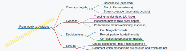
Example: turning the matrix into a flight readiness plan
Once the matrix exists, you can define a repeatable readiness flow:
- Before integration: run acceptance tests on the specific unit (subset duty + leak/performance checks).
- After flight: perform inspection and compare to the trending curves established in qualification.
- If metrics drift: apply the rework path or escalate inspection scope.
The matrix is what makes these steps consistent across hardware lots and across time.
Common pitfalls to avoid
- Testing the wrong stressors: if erosion is driven by a specific flow regime, don’t rely on a generic duty cycle.
- No linkage to acceptance evidence: qualification without acceptance metrics leads to “we proved it once” but no practical screening.
- Overly broad coverage targets: if every mechanism gets the same test time, you’re likely wasting effort on low-risk items.
- No trending plan: end-point checks hide degradation rates, which are often the real decision input.
A good test matrix is not just a schedule. It is a decision system that connects damage mechanisms to measurable evidence, then converts that evidence into clear go/no-go outcomes for reused hardware.
9. Reliability Engineering and Failure Management Across Flights
9.1 Apply Reliability Modeling With Example FMEA and Fault Tree Inputs
Reliability modeling is where “it failed once” turns into “it fails in a way we can quantify and prevent.” For reusable launch systems, the modeling inputs must reflect repeated duty: multiple hot-fire cycles, reentry heating, landing loads, inspection/repair, and reassembly. The goal is not to predict the future perfectly; it’s to build a model that is consistent with known failure mechanisms and that produces actionable maintenance and design decisions.
Start with the reliability boundary and mission phases
Before any FMEA or fault tree, define the system boundary and the time windows that matter. A common mistake is mixing failure modes from different phases (ascent vs. landing) without accounting for different stressors.
Example boundary for a reusable first-stage engine system:
- Ascent propulsion: ignition through main cutoff.
- Stage recovery: coast, restart (if applicable), landing burn.
- Post-flight handling: inspection, repair, reassembly.
Each phase gets its own failure-rate or probability model inputs, because the dominant causes differ.
Build the FMEA: failure modes, effects, and detection
FMEA (Failure Modes and Effects Analysis) turns component-level failure mechanisms into system-level consequences. For reliability modeling, you want FMEA entries that are specific enough to map to fault tree basic events and to maintenance actions.
A practical FMEA template for reusable hardware includes:
- Item (e.g., turbopump bearing, valve actuator, controller power supply)
- Function (e.g., “deliver propellant at commanded flow”)
- Failure mode (e.g., “stuck closed valve,” “bearing seizure,” “sensor bias causing wrong control output”)
- Immediate effect (e.g., “reduced flow,” “overpressure,” “loss of control authority”)
- End effect (e.g., “engine shutdown,” “thrust decay,” “vehicle loss”)
- Detection (e.g., “telemetry threshold,” “built-in test,” “post-flight inspection finding”)
- Controls (design features, procedures)
- Occurrence basis (how you estimate frequency: life-limited cycles, test data, or field history)
Example FMEA entries (engine valve and sensor)
Below are two FMEA entries that are intentionally written to support later fault tree mapping.
| Item | Function | Failure mode | Immediate effect | End effect | Detection | Occurrence basis |
|---|---|---|---|---|---|---|
| Main oxidizer valve actuator | Open/close on command | Stuck closed | Oxidizer flow starvation | Thrust decay / engine shutdown | Commanded vs. measured position mismatch | Valve cycle life model + test wear data |
| Chamber pressure sensor | Provide pressure feedback | Bias high | Controller commands reduced mixture ratio | Overcooling/underperformance or instability | Pressure residuals vs. model | Sensor calibration drift model + inspection results |
Notice what’s missing: vague wording like “actuator failure.” The failure mode is specific enough to decide whether the mitigation is a different actuator design, a different sensor, a better diagnostic threshold, or a different inspection interval.
Convert FMEA to fault tree inputs
A fault tree starts with a top event (e.g., “engine fails to achieve required thrust during ascent”) and decomposes it into combinations of basic events. The basic events should align with FMEA failure modes or with groups of failure modes that share the same cause.
A good mapping rule:
- If an FMEA entry has a clear immediate effect and detection/controls, it can usually become a basic event.
- If multiple FMEA entries share a single underlying cause (e.g., “contamination in valve seat”), group them into an intermediate event.
Example fault tree: engine thrust shortfall
Top event: Engine thrust shortfall during ascent.
Key contributors (illustrative):
- Oxidizer flow low (valve stuck closed)
- Fuel flow low (pump cavitation or valve restriction)
- Control loop drives mixture ratio out of bounds (sensor bias)
- Ignition/combustion instability leading to shutdown (thermal or mixture issues)
    flowchart TD
  A[Top: Thrust shortfall during ascent] --> B[Oxidizer flow low]
  A --> C[Fuel flow low]
  A --> D[Mixture ratio control error]
  A --> E[Early shutdown]

  B --> B1[Oxidizer valve stuck closed]
  B --> B2[Oxidizer valve leakage / partial closure]

  C --> C1[Fuel valve restriction]
  C --> C2[Pump cavitation due to low inlet pressure]

  D --> D1[Chamber pressure sensor bias high]
  D --> D2[Flow sensor bias / calibration drift]
  D --> D3[Controller software logic fault]

  E --> E1[Combustion instability leading to cutoff]
  E --> E2[Overtemperature protection triggers]
Assign probabilities: from occurrence to conditional likelihood
Reliability modeling needs numbers. For launch systems, you often combine:
- Occurrence probability for a failure mode (from life models or test data)
- Conditional probability that the failure mode leads to the top event (given detection/controls)
A simple structure for a basic event \(i\): \[ P(\text{Top}) \approx \sum_i P(i),P(\text{Top} \mid i) \] This is not exact for all dependencies, but it’s a useful first pass. The fault tree then refines logic (AND/OR) and dependencies.
Example: valve stuck closed with diagnostic coverage
Suppose the FMEA indicates:
- Valve stuck closed probability per flight: \(P(\text{stuck}) = 2\times 10^{-4}\)
- Diagnostic coverage: the system detects the mismatch and triggers a safe shutdown before thrust falls below the required threshold with probability (c = 0.7)
If “thrust shortfall” is defined as failing to meet thrust requirements before shutdown, then: \[ P(\text{Top} \mid \text{stuck}) = 1 - c = 0.3 \] So the contribution is: \[ P(\text{Top}) \approx (2\times 10^{-4})(0.3)=6\times 10^{-5} \] This is the kind of calculation that forces clarity: what exactly counts as “shortfall,” and how much time does detection buy you?
Include reusability effects in the modeling inputs
Reusable systems change the input distributions because the hardware state evolves across flights.
Common modeling adjustments:
- Cycle-dependent failure rates: occurrence increases after certain hot-fire cycles.
- Repair-induced variability: after inspection and repair, the failure probability may reset partially, not fully.
- Inspection effectiveness: detection in FMEA should reflect what inspection actually finds (false negatives matter).
A practical way to represent this is to parameterize basic event probability by flight count (n): \[ P(i\mid n) = f_i(n) \] Then the mission-level probability becomes a sum over the relevant flights or a weighted average if you model a fleet.
Use FMEA severity and fault tree logic consistently
FMEA often includes severity ranking, but reliability modeling needs a consistent mapping from severity to probability of reaching the top event.
A consistency check:
- If FMEA severity is “catastrophic,” the fault tree should route that failure mode toward the top event unless there is a credible mitigation path.
- If FMEA severity is “major” but the fault tree top event is “vehicle loss,” then the fault tree should include additional logic (e.g., “major failure plus secondary failure”).
This avoids a common mismatch where FMEA severity is high but the fault tree top event is narrowly defined.
Example workflow: from FMEA entry to model contribution
- Select top event: “engine thrust shortfall during ascent.”
- Create FMEA entries for likely contributors: valve stuck closed, sensor bias, pump cavitation.
- Map FMEA to fault tree: each entry becomes a basic event or intermediate event.
- Quantify occurrence: use cycle-based failure probability per flight.
- Quantify conditional likelihood: incorporate diagnostic coverage and control actions.
- Compute top event probability using fault tree logic (AND/OR) and basic event probabilities.
- Feed results back: if a basic event dominates, decide whether to change design, diagnostics thresholds, inspection criteria, or maintenance intervals.
Mind map: reliability modeling inputs and flow
What “good inputs” look like
Good FMEA and fault tree inputs share three traits:
- They are phase-aware (ascent vs. recovery vs. post-flight).
- They are decision-aware (detection and controls are explicit, not implied).
- They are state-aware (cycle count and repair/inspection outcomes affect probabilities).
When those traits are present, reliability modeling stops being a spreadsheet exercise and becomes a structured way to connect hardware behavior to operational decisions—without pretending the math is magic.
9.2 Set Maintenance Actions Based on Condition Monitoring With Example Thresholds
Condition monitoring only helps if it turns into consistent actions. The trick is to define thresholds that map measurable signals to maintenance decisions, then to verify those decisions actually reduce risk and turnaround time. Below is a practical way to do it for reusable launch hardware, with example thresholds you can adapt.
Start with a maintenance decision ladder
Create a small set of action levels that cover what you can realistically do between flights. A typical ladder looks like this:
- Level 0: No action (monitor only)
- Level 1: Inspect (targeted checks)
- Level 2: Repair/replace (restore to “as-new” or “as-qualified”)
- Level 3: Remove from service (hardware is not eligible for another flight)
Then define what “inspect,” “repair,” and “remove” mean in terms of work scope, required tools, and acceptance criteria. If Level 1 is “inspect,” specify which inspection method and what pass/fail thresholds are used.
Use condition monitoring signals that correlate to failure modes
Pick signals that connect to known degradation mechanisms. Examples for reusable systems:
- Vibration signatures → bearing wear, imbalance, looseness
- Valve actuation current/latency → friction, sticking, seal wear
- Thermal soakback rates → insulation degradation, heat path changes
- Pressure/flow transients → cavitation damage, injector fouling
- Structural strain residuals → loosened mounts, plastic deformation
A useful sanity check: if a signal changes but the failure mode doesn’t, you’ll waste maintenance. If the failure mode changes but the signal doesn’t, you’ll miss maintenance. Aim for signals that do both.
Define thresholds using three bands: normal, caution, and action
For each monitored parameter, define:
- Normal band: expected variation across flights and environments
- Caution band: indicates drift toward a known degradation mechanism
- Action band: indicates unacceptable risk or loss of performance margin
You can implement this with either absolute thresholds, rate-of-change thresholds, or both.
Example: engine valve health thresholds
Assume you monitor a set of identical valves and record actuation latency (time from command to achieved position) and actuation current (peak current during motion). You also know from test data that sticking begins to appear when latency rises.
Example thresholds (per valve):
- Normal: latency ≤ 120 ms and peak current ≤ 1.05× baseline
- Caution (Level 1): 120–140 ms OR 1.05–1.15× baseline
- Action (Level 2): 140–160 ms OR 1.15–1.25× baseline
- Remove (Level 3): >160 ms OR >1.25× baseline
Add a rate-of-change rule to catch sudden issues:
- If latency increases by ≥ 15 ms compared to the previous flight, treat as Level 2 regardless of absolute value.
Why this works: baseline-relative thresholds handle manufacturing spread and temperature effects, while rate-of-change catches anomalies that absolute thresholds might miss.
Example: turbopump bearing vibration thresholds
Suppose you track 1× and 2× shaft-order vibration RMS during a standardized operating segment. You also compute a trend slope over the last three flights.
Example thresholds:
- Level 0: RMS ≤ 3.0 mm/s and trend slope ≤ +0.2 mm/s per flight
- Level 1 (inspect): RMS 3.0–3.8 mm/s OR slope +0.2 to +0.5 mm/s per flight
- Level 2 (repair/replace): RMS 3.8–4.5 mm/s OR slope > +0.5 mm/s per flight
- Level 3 (remove): RMS > 4.5 mm/s OR any spike > 20% above the last flight during the same segment
A practical note: vibration is sensitive to operating conditions. Make sure the monitored segment is defined by thrust level, mixture ratio, and rotational speed window, so you’re comparing like with like.
Example: thermal protection inspection triggers
For reusable thermal protection, you might monitor surface temperature during a standardized entry and post-flight mass loss or heat flux proxy. If you can’t measure the same physical quantity every time, use a proxy that still correlates with damage.
Example thresholds for a tile segment:
- Level 0: peak heat flux proxy ≤ 1.00× predicted and no visible cracking beyond baseline
- Level 1 (inspect): 1.00–1.10× predicted OR visible cracking within a defined size range
- Level 2 (repair): 1.10–1.20× predicted OR cracking exceeds the size range OR delamination area exceeds a set limit
- Level 3 (remove): >1.20× predicted OR delamination exceeds the maximum allowable area OR repeated Level 2 triggers on the same segment
This is where “repeatability” matters: define the inspection method and measurement tools so that Level 1 and Level 2 decisions don’t depend on who did the work.
Mind map: condition monitoring to maintenance actions
Mind map: Maintenance actions from condition monitoring
Turn thresholds into work instructions (not just numbers)
A threshold without a defined work package causes inconsistency. For each action level, specify:
- Who performs the work (roles)
- What is done (inspection method, repair steps)
- Where it is done (component location, subsystem boundaries)
- How it is verified (acceptance tests)
- What documentation is updated (as-built records, serial traceability)
Example for Level 1 valve inspection:
- Remove actuator cover
- Perform visual inspection for seal wear and scoring
- Measure stem friction proxy using a standardized test
- Acceptance: friction proxy within X% of baseline and no scoring beyond Y mm
If you don’t define the acceptance criteria, the threshold becomes a suggestion.
Control false positives and false negatives with two extra rules
- Require persistence for slow degradation. If a parameter drifts gradually, trigger Level 1 only after it persists for two consecutive flights (or two consecutive test segments). This prevents maintenance from chasing noise.
- Allow immediate escalation for sudden anomalies. If a parameter jumps sharply, escalate immediately even if it’s still within the caution band. Sudden changes often indicate a different mechanism than slow wear.
Use a simple threshold table template
| Parameter | Normal | Level 1 (Inspect) | Level 2 (Repair) | Level 3 (Remove) | Rate rule |
|---|---|---|---|---|---|
| Valve latency (ms) | ≤120 | 120–140 | 140–160 | >160 | +15 ms vs prev flight |
| Peak current (×baseline) | ≤1.05 | 1.05–1.15 | 1.15–1.25 | >1.25 | N/A |
| Bearing vib RMS (mm/s) | ≤3.0 | 3.0–3.8 | 3.8–4.5 | >4.5 | +20% spike |
Close the loop: verify thresholds against outcomes
After each flight and maintenance cycle, compare what you predicted with what you found. Track:
- False positives: you inspected/removed but found no actionable degradation
- False negatives: you flew again and later discovered damage that should have triggered an earlier action
- Turnaround impact: how often Level 2 or Level 3 actions occurred and how long they took
When false positives are high, tighten the persistence rule or improve normalization. When false negatives appear, revisit correlation between the signal and the failure mode, and adjust thresholds or add a new signal.
Condition monitoring becomes valuable when it behaves like a disciplined interface: signals in, thresholds and decision logic, defined work out, and measurable feedback back into the thresholds. That’s the difference between “we measured something” and “we prevented a bad day.”
9.3 Handle Anomalies With Example Root Cause and Corrective Action Loops
An anomaly is any deviation that matters: a sensor disagrees with expected behavior, a valve response is slower than modeled, a landing burn ends early, or a reused component shows a pattern that wasn’t present on the first flight. The goal of the loop is simple: detect → contain → diagnose → correct → prevent recurrence, while preserving evidence for later reuse decisions.
A practical anomaly loop (what to do in what order)
-
Detect and classify
- Use thresholds tied to flight rules, not just “out of family” statistics.
- Classify as transient, degrading, or hard failure based on whether the behavior returns to normal, trends, or stops.
-
Contain and protect the mission
- Freeze the configuration that could mask the cause (e.g., stop additional parameter changes once you see the deviation).
- Switch to a safe mode if continuing would increase damage or destroy diagnostic value.
- Record the exact timeline: event start, guidance mode, actuator commands, and any operator actions.
-
Preserve evidence
- Lock down raw telemetry, event logs, and health-monitor outputs.
- Save the exact software build, parameter set, and calibration tables used for that flight.
- If hardware is recovered, tag it immediately with flight ID and anomaly category.
-
Diagnose with a structured root cause method
- Start with a fault tree or FMEA-linked hypothesis list so you don’t “invent” explanations.
- Use a “most likely, least invasive” approach: verify the simplest checks first (wiring, connector seating, calibration drift, software parameter mismatch).
-
Correct with measurable actions
- Separate fixing the symptom from fixing the cause.
- For each corrective action, define: owner, due date, verification method, and what evidence will prove the cause is addressed.
-
Prevent recurrence via design, process, and verification changes
- Update inspection criteria, maintenance procedures, test coverage, and acceptance limits.
- Ensure the change is configuration-controlled so the next flight actually uses it.
-
Close the loop
- Confirm the corrective action’s effectiveness on the next relevant test or flight.
- If the anomaly is tied to reuse, update life limits or inspection intervals based on observed degradation.
Mind map: anomaly handling loop
Example 1: Reused engine valve shows slower response
Observed anomaly: During a reused stage flight, the oxidizer valve reaches commanded position later than the expected actuator response curve. The guidance system compensates, but the margin to the next event shrinks.
Containment: Operators keep the valve control law unchanged and avoid additional tuning mid-flight. The system logs the actuator command history and the valve position sensor readings at high rate.
Evidence preserved:
- Telemetry: command vs position, time-to-position, and any controller saturation flags.
- Ground data: last post-flight checkout results and maintenance records.
- Hardware: valve assembly serial number, actuator coil resistance readings, and any prior inspection findings.
Diagnosis (root cause reasoning):
- Hypothesis A: sensor calibration drift.
- Hypothesis B: actuator friction increase due to contamination.
- Hypothesis C: electrical supply degradation (connector resistance, harness damage).
A quick check shows the position sensor output is consistent with a separate diagnostic channel during bench tests. The actuator coil resistance is slightly higher than the baseline, and inspection finds a connector with oxidation at a pin interface.
Root cause: Increased electrical resistance at the connector caused reduced actuator force, slowing the valve response. The connector degradation was not caught by the previous inspection criteria.
Corrective action loop:
- Correct: Replace connector hardware with a revised part and apply an updated mating procedure (cleaning + torque spec + visual criteria).
- Verify: Run an actuator response test on representative hardware to confirm time-to-position returns to baseline within tolerance.
- Prevent recurrence:
- Update inspection checklist to include connector surface condition and resistance measurement.
- Add a bench test step to measure actuator response after refurbishment.
- Ensure the maintenance procedure is configuration-controlled so it applies to all reused units.
Closure: On the next flight, the valve response time stays within the tightened acceptance band, and the guidance margin remains stable.
Example 2: Guidance mode switching causes a transient attitude error
Observed anomaly: After a stage separation event, the vehicle briefly enters a different guidance mode than expected, producing a short attitude error spike. The spike is within control authority, but it correlates with a specific configuration state.
Containment: The flight software does not accept new mode-change commands during the transient window. This prevents “chasing” the error and preserves a clean cause-effect timeline.
Evidence preserved:
- Mode transition logs with timestamps.
- Configuration state variables (e.g., sensor validity flags, estimator selection signals).
- Software build hash and parameter set.
Diagnosis:
- Hypothesis A: estimator selection logic uses a sensor validity flag that is momentarily wrong.
- Hypothesis B: a parameter mismatch exists between ground and flight configuration.
- Hypothesis C: a timing race condition in the mode transition logic.
The mode transition log shows the sensor validity flag toggles for a few hundred milliseconds right after separation. The raw sensor data indicates a brief dropout consistent with a connector vibration or a power rail dip. Ground tests reproduce the dropout when the harness is routed in the same way.
Root cause: A harness routing and strain-relief detail allowed micro-movement at separation, causing a momentary sensor power interruption.
Corrective action loop:
- Correct: Rework strain relief and add a retention feature to prevent movement at separation.
- Verify: Conduct a vibration test or harness motion test that replicates separation-induced motion, then confirm sensor validity flags remain stable.
- Prevent recurrence:
- Update assembly procedure with a measurable routing constraint.
- Add a pre-flight harness inspection step that checks the retention feature and performs a functional sensor validity check.
- Expand the test matrix to include the exact configuration state used during separation.
Closure: Subsequent flights show no attitude spike at the same event, and the mode transition sequence matches the expected state machine.
Example 3: Thermal protection inspection finds a pattern of edge cracking
Observed anomaly: After recovery, thermal protection tiles show edge cracking concentrated near a specific boundary line. The cracking is not catastrophic, but it appears repeatedly across reused vehicles.
Containment: The hardware is quarantined for inspection beyond the normal scope so the team can map crack locations relative to airflow and structural interfaces.
Evidence preserved:
- High-resolution images with a consistent coordinate system.
- Tile location, thickness, and installation details.
- Flight thermal data: heating rate estimates and local temperature proxies.
Diagnosis:
- Hypothesis A: installation stress from tile fastening method.
- Hypothesis B: local thermal gradient higher than predicted.
- Hypothesis C: coating or bondline aging due to repeated thermal cycling.
Crack locations align with a structural interface that experiences higher-than-modeled differential expansion. The bondline inspection shows early degradation at the same boundary.
Root cause: Differential expansion at the interface increased bondline shear stress, accelerating cracking over repeated cycles.
Corrective action loop:
- Correct: Modify the interface design or bondline material stack to reduce shear stress (e.g., compliant layer or revised bondline thickness).
- Verify: Perform thermal cycling tests that reproduce the measured gradient and then inspect for crack initiation and growth.
- Prevent recurrence:
- Update inspection thresholds to flag early edge cracking before it reaches a critical size.
- Add a refurbishment step that checks bondline condition at the interface.
- Record the change in the configuration management system so reused hardware is treated consistently.
Closure: Cracking shifts from “repeatable pattern” to “rare and within acceptance,” and the reuse decision becomes more stable.
A compact checklist for writing the corrective action
For each anomaly, ensure the corrective action statement includes:
- Cause: the specific mechanism (not just “sensor issue”).
- Action: what changes in hardware or process.
- Verification: how you prove it worked (test, inspection, or analysis).
- Acceptance: the measurable criterion.
- Propagation: which configurations, serial ranges, and refurbishment steps are updated.
When this checklist is followed, the loop stops being a report and becomes an engineering mechanism—one that makes reuse safer because it turns “what happened” into “what we will do differently next time.”
9.4 Define Spare Strategy and Repair Levels With Example Logistics Constraints
A reusable launch system only stays “reusable” if you can keep it flying on schedule. Spare strategy and repair levels are the practical bridge between engineering design and the reality of turnaround windows, transport limits, and inspection throughput.
1) Start with the logistics constraints that actually bite
Before choosing spares, write down the constraints that will govern decisions. A good starting set:
- Turnaround window: how many hours/days you have between landing and next launch.
- Inspection capacity: number of NDE stations, technicians, and shift coverage.
- Repair lead time: longest time to replace, machine, cure, or requalify a repaired item.
- Transport and handling: whether the spare must travel with the vehicle or can be shipped later.
- Shelf life and storage: especially for electronics, seals, propellant-contact materials, and adhesives.
- Test access: whether you can run acceptance tests immediately or only at specific facilities.
Example constraint set (stage avionics bay):
- Turnaround window: 72 hours.
- NDE stations: 1 for the bay, 2 for subcomponents.
- Repair lead time (worst case): 36 hours for harness replacement plus 12 hours for curing/verification.
- Acceptance test: requires a specific bench available only during day shift.
From this, you can already see that “repair everything” is not a plan; you need spares that reduce the time spent waiting for repairs.
2) Define repair levels as a decision ladder
Repair levels should be explicit and mutually exclusive. A common structure is:
- Level 0: No repair (replace only). Used when repair would require disassembly beyond what’s safe or when inspection cannot confirm integrity.
- Level 1: Field repair (limited disassembly, replace modules, verify). Used when you can swap a line-replaceable unit (LRU) and run a quick functional test.
- Level 2: Shop repair (full disassembly, component replacement, bench testing). Used when you need controlled processes like machining, rework, or calibration.
- Level 3: Depot repair (special tooling, deeper refurbishment, possible redesign of subassemblies). Used when the item is life-limited or when damage is complex.
Example (turbopump bearing cartridge):
- Level 0: If scoring exceeds a threshold, replace cartridge; no field repair.
- Level 2: If wear is within limits, disassemble, replace bearings, re-balance, and run bench tests.
- Level 3: If housing damage is present, send to depot for inspection and potential refurbishment.
The key is that each level must specify: what actions are allowed, what inspections are required, and what tests prove “ready for flight.”
3) Choose spares categories that match failure modes
Spare strategy works best when it’s organized by why you need spares, not just by part number.
- Operational spares: items you expect to replace due to normal wear or post-flight inspection outcomes.
- Contingency spares: items you keep to cover low-probability but high-impact failures that would otherwise break the schedule.
- Test spares: items reserved for acceptance testing, calibration, or qualification checks.
- Repair pipeline spares: items that keep the vehicle moving while repaired units cycle through Level 2/3.
Example (thermal protection tiles on a reusable fairing):
- Operational spares: tiles that are routinely replaced when inspection flags edge chipping.
- Contingency spares: a small set of tiles for worst-case impact zones that would otherwise halt processing.
- Repair pipeline spares: tiles held so the fairing can be assembled while the “repaired tile lot” is being processed.
4) Use a simple logistics math model to size spares
You don’t need a full stochastic simulation to make good decisions. A practical approach is to compute the number of spares needed to cover expected replacements plus schedule risk.
Let:
- (N) = number of flights in the planning horizon.
- (p) = probability an item requires replacement after a flight (based on inspection outcomes and known failure/repair triggers).
- (L) = average number of items in the repair pipeline at any time.
- (S) = spare quantity you must have on hand.
A basic sizing target is: \[ S \ge N\cdot p + L \]
Then you add a buffer for schedule-critical items where the cost of missing a launch is higher than the cost of carrying extra spares.
Example (LRU avionics computer):
- Planning horizon: (N=10) flights.
- Probability of replacement after inspection: (p=0.08).
- Repair pipeline average: (L=1) (because Level 2 turnaround takes time).
Compute expected replacements: \( 10\cdot 0.08=0.8 \). Add pipeline: (0.8+1=1.8). Round up to 2 spares for the baseline.
Now consider schedule criticality. If the launch window is tight and bench testing is a bottleneck, you might carry 1 additional contingency unit, resulting in (S=3).
5) Mind map: spare strategy and repair levels with logistics constraints
6) Example: mapping repair levels to spares under a tight turnaround
Consider a reusable first-stage hydraulic power unit (HPU) with the following realities:
- Post-flight inspection flags a subset of HPUs for replacement due to seal wear.
- Level 1 repair (seal kit swap) is possible in 8 hours but requires a specific torque procedure and a pressure test.
- Level 2 repair (pump rework) takes 2.5 days and needs a shop bench.
- Level 0 replacement is required if contamination is found beyond a threshold.
Logistics constraints:
- Turnaround window: 72 hours.
- Pressure test bench: available for only 1 shift per day.
- Shop bench: available 5 days/week.
Decision mapping:
- If contamination is severe (Level 0), you must swap the HPU immediately and send the unit to Level 2/3.
- If seal wear only (Level 1), you can repair in-place if the pressure test slot is available.
Spare plan:
- Keep enough HPUs to cover Level 0 swaps and to prevent waiting for Level 2.
- Keep seal kits as Level 1 spares, but only if the pressure test bench is not the limiting resource.
Concrete outcome:
- If the pressure test bench is the bottleneck, you carry more complete HPU spares rather than relying on Level 1 repairs.
- If the bench is plentiful, you reduce HPU spares and increase seal kit spares.
This is the core idea: spares are not just “extra parts.” They are a way to route around the slowest step in the process.
7) Repair levels must include “proof of readiness”
A repair level without verification is just maintenance theater. Each level should define:
- Inspection triggers: what measurements decide Level 0 vs Level 1 vs Level 2.
- Repair actions allowed: what can be replaced or reworked.
- Verification tests: what must be run to declare the item flight-ready.
- Documentation outputs: what records are required for traceability.
Example (LRU harness replacement):
- Level 1 allows connector replacement and harness re-termination.
- Verification includes continuity checks, insulation resistance, and a functional test in the relevant mode.
- If any test fails, the item is escalated to Level 2 (not “fixed later”).
8) Configuration and traceability: spares must be interchangeable in practice
Even if two parts are “the same,” they may not be interchangeable due to software versions, calibration states, or mechanical revision differences.
A spare strategy should therefore include:
- Serialization and traceability: each spare’s history and configuration state.
- Compatibility rules: what revisions can be swapped without additional rework.
- Acceptance criteria: what tests confirm the spare is ready in the current configuration.
Example:
- A reused sensor may require updated calibration coefficients after a repair level change.
- If you treat it as a drop-in spare without calibration verification, you risk a “ready” tag that isn’t actually true.
9) Practical checklist for defining spares and repair levels
- Identify the slowest steps in turnaround (inspection, bench tests, curing, transport).
- Define Level 0/1/2/3 with allowed actions and required verification.
- Classify spares by operational, contingency, test, and pipeline roles.
- Size baseline spares using \( S \ge N\cdot p + L \), then add buffer for schedule-critical items.
- Ensure spares are truly interchangeable via configuration and traceability rules.
- Validate the plan with a “worst-case day” walkthrough: what happens if the inspection flags the maximum number of items that day?
When this is done well, the system doesn’t just survive reuse—it stays on schedule while doing it. That’s the part engineers can measure, improve, and defend.
10. Quality Assurance, Configuration Management, and Documentation
10.1 Implement Configuration Control for Reused Hardware and Software
Configuration control is what keeps “reused” from turning into “mystery meat.” When hardware and software come back for another flight, you need a system that answers three questions every time: What exactly is this? What changed since last flight? And what evidence says it’s safe to use again?
What configuration control must cover
Configuration control is not just paperwork. It is the end-to-end discipline that ties together physical items, software artifacts, and the rules for how they may be assembled and flown.
1) Define the configuration items (CIs)
Start by listing what you will control as a CI. Typical CIs for reusable launch systems include:
- Reused flight hardware: engines, avionics boxes, tanks, interstages, landing legs, thermal protection panels.
- Software items: flight software build, ground software version, configuration parameters, and mission scripts.
- Documentation items that affect build/verification: interface control documents, wiring diagrams, inspection procedures, and test acceptance criteria.
A practical habit: if a change could alter mass, interfaces, thermal behavior, loads, or fault handling, it belongs in the CI list.
2) Establish baselines
A baseline is a named snapshot of a CI set that is known to work together. For reuse, you usually need at least:
- A “design baseline” (what the item was originally built to).
- A “flight baseline” (what was actually assembled and verified for a specific flight).
- A “current baseline” for each reused item after inspection and any approved repairs.
Example: If an engine controller software build is updated, the flight baseline must record which hardware serials it was paired with, not just the software version.
3) Control changes with clear authority
Changes should flow through a defined path with named decision makers. A common failure mode is informal approvals (“it looks fine”) that never become part of the controlled record.
A workable rule set:
- Engineering change request (ECR) describes the reason, scope, and affected CIs.
- Configuration control board (CCB) approves or rejects based on impact analysis.
- Verification plan states what evidence is required before the changed CI can be used.
The configuration control workflow (with reuse-specific checkpoints)
A reuse cycle has extra pressure points: inspection outcomes, repairs, and reassembly. Your workflow should explicitly gate those steps.
Step A: Identify the item and its history
Every reused CI should carry a unique identity (serial number, asset tag, or traceable identifier). The configuration record should include:
- Build baseline reference
- Repair history entries (what was replaced, what was reworked)
- Inspection results and any deviations
- Software pairing history (for avionics and controllers)
Example: A reused avionics box might pass inspection but have a connector replacement. The configuration record must show the connector part number and the inspection procedure used after replacement.
Step B: Determine “as-found” configuration
Before you disassemble or repair, capture the as-found state. This can be as simple as:
- Photographic evidence of installed components
- Measured values (torque marks, resistance checks, leak checks)
- Software hashes or build identifiers
Why it matters: if you only record “as-left” after repairs, you lose the ability to explain why a later anomaly happened.
Step C: Apply approved changes only
Repairs and modifications must be either:
- Within an approved repair scheme (pre-authorized actions with known verification), or
- Treated as a change requiring ECR/CCB approval.
Example: If a thermal protection panel has a known allowable rework method, you can use the approved scheme. If the rework requires a different adhesive lot or a different panel geometry, treat it as a change.
Step D: Verify and update the configuration record
After inspection and any repairs, update the configuration record to reflect the current baseline. Evidence should link to the CI:
- Inspection report IDs
- Test results IDs
- Software build identifiers
- Hardware part numbers and serials
A good sanity check: someone reading the record should be able to reconstruct the assembly without asking the shop floor.
Mind map: configuration control for reused hardware and software
Examples that show the difference between “version” and “configuration”
Example 1: Software version changes without configuration control
Scenario: A ground operator updates a parameter file to adjust a sensor scaling. The flight software build stays the same.
If you only record “software version,” you miss the parameter file content. Configuration control should treat parameter sets as configuration items or as controlled artifacts with hashes.
Outcome: The configuration record must show the parameter file identifier and the exact hash used for that flight.
Example 2: Hardware serials swapped during refurbishment
Scenario: Two reused actuators are refurbished in parallel. One passes inspection; the other fails and is repaired.
If the shop floor uses only part numbers, you can accidentally assemble the repaired actuator into the wrong stage. Configuration control prevents this by:
- Requiring serial-level traceability
- Updating the current baseline only after verification
- Blocking release if the expected serial does not match the record
Outcome: The flight baseline ties the actuator serial to the stage assembly and the verification evidence.
Example 3: Approved repair scheme used outside its limits
Scenario: A repair procedure allows replacing a connector under certain conditions (e.g., specific connector family and measured resistance range). A team uses the procedure but the measured resistance is outside the allowed range.
Configuration control should catch this because the procedure’s applicability conditions are part of the controlled documentation. The record should either:
- Route the case to an ECR, or
- Require a documented deviation with CCB approval and additional verification.
Outcome: You preserve the integrity of the evidence chain.
Configuration status accounting: the “what’s released” view
Engineers need a clear answer to: what is released for flight right now?
A minimal status record for each stage assembly might include:
- Stage assembly ID
- List of installed CIs with serials/part numbers
- Software build ID and parameter set ID
- Inspection/test evidence IDs
- Release status (released / hold / pending)
Example rule: a CI cannot be marked “released” unless its evidence links are present and complete. This prevents the classic “we’ll add the paperwork later” problem.
Practical implementation details that reduce drift
- Use immutable identifiers for software artifacts (build IDs and hashes) so “same version” can’t hide different content.
- Require part/serial pairing at integration time, not after the fact.
- Keep documentation under configuration control so the inspection procedure used is the one recorded.
- Make the configuration record update a gated step in the workflow, not an optional admin task.
Quick checklist for engineers and integration leads
- Do we know the exact CI set for the current baseline?
- Are hardware serials and software hashes recorded together?
- Are repairs either within approved schemes or formally changed?
- Is the release status tied to evidence IDs?
- Can someone reconstruct the assembly from the record alone?
When configuration control is done well, reuse becomes a repeatable engineering process rather than a series of careful guesses. The goal is simple: the next flight should be explainable with the same clarity as the first.
10.2 Use Traceability Practices With Example Part Numbering and Serialization
Traceability is what lets you answer, quickly and confidently, “What exactly flew?” and “What changed since the last flight?” In reusable launch systems, that question matters because hardware is reused, repaired, inspected, and reassembled on a schedule. If traceability is weak, you end up with expensive ambiguity: you can’t tell whether a recurring issue is tied to a specific component, a specific repair, or a specific processing batch.
A practical traceability system ties together four things:
- Identity (what the item is): part number, serial number, and configuration.
- History (what it has experienced): manufacturing lots, inspections, repairs, and test results.
- Configuration (what it was assembled as): software versions, hardware options, and interface states.
- Disposition (what it is allowed to do now): acceptance status, life limits, and maintenance actions.
The traceability chain: from drawing to flight
A good rule of thumb is to ensure every “decision point” has an identifier you can reference later. For example:
- When a component is received, record its serial number and inspection results.
- When it is repaired, record the repair procedure ID and the resulting inspection outcomes.
- When it is assembled, record the assembly configuration and the mating interface identifiers.
- When it is released for flight, record the release authority and the applicable acceptance criteria.
If you do this consistently, you can reconstruct the chain of custody without relying on memory or spreadsheets with missing columns.
Part numbering: make it structured, not just unique
Part numbers should help humans and systems locate the right item quickly. A common approach is to encode key attributes into the part number while keeping a separate serial number for the unique physical item.
Here’s an example part numbering scheme for a reusable engine valve assembly:
- AA-BB-CCCC-DDD-E
- AA: subsystem (e.g., EN for engine)
- BB: component family (e.g., VA for valve)
- CCCC: base design number
- DDD: variant or configuration (e.g., 102)
- E: revision level (e.g., A, B, C)
Example:
- EN-VA-1842-102-C
This part number tells you the design intent and revision. It does not tell you which physical valve you have. That’s the serial number’s job.
Serialization: unique identity for the physical item
A serial number should be unique across the life of the item and stable across moves between facilities. It should also be easy to print and scan.
Example serial format:
- SN-YYYY-LL-SSSS
- YYYY: year of manufacture
- LL: production line or cell
- SSSS: sequential number
Example:
- SN-2024-03-0197
Now you can record: “Valve assembly EN-VA-1842-102-C, serial SN-2024-03-0197.” That combination is usually enough to locate the item’s history.
Configuration control: don’t confuse “part” with “as-built”
Reusable systems often have multiple layers of configuration:
- Hardware configuration: which variant of a part is installed.
- Interface configuration: which mating hardware, gaskets, fasteners, or adapters.
- Software configuration: which firmware build and parameter set.
A common failure mode is treating the part number as if it fully describes the as-built state. It doesn’t. Two items with the same part number can be assembled with different interface kits or different software parameter sets.
To address this, record an assembly configuration ID at the time of integration. Example:
- CFG-BOOSTER-07-2026-0315
This ID points to a configuration record that lists:
- installed component serial numbers
- interface kit serials
- software build IDs
- acceptance test results
Traceability data model: what to store and where
You don’t need a complicated database design to start, but you do need consistent fields. A minimal traceability record for a serialized component can include:
part_numberserial_numberlot_or_batch(if applicable)manufacturing_siteinspection_results(with test IDs)repair_events(each with procedure ID and outcome)life_usage(cycles, hot-fire hours, thermal exposures)current_status(released, quarantined, scrapped)linked_assemblies(assembly configuration IDs)
For assemblies, store:
assembly_idassembly_type(e.g., stage, engine module)installed_components(serial numbers)interface_states(torque/fit checks, gasket part serials)software_configuration_idacceptance_tests(with pass/fail and evidence IDs)
Mind map: traceability practices for reusable hardware
Example: end-to-end traceability for a reused engine valve
Assume a valve assembly is installed in an engine module for flight F-12.
-
Receiving
- Part: EN-VA-1842-102-C
- Serial: SN-2024-03-0197
- Evidence: inspection report
IR-2024-1198(pass)
-
Repair (optional)
- Repair event: procedure
RP-VALVE-07 - Date: 2025-09-14
- Evidence: NDE report
NDE-25-441(pass)
- Repair event: procedure
-
Integration
- Assembly configuration:
CFG-ENGMOD-03-2026-0315 - Installed serial list includes SN-2024-03-0197
- Interface kit serial:
KIT-IF-55-0008
- Assembly configuration:
-
Flight readiness
- Release record:
FRR-2026-0315(released) - Acceptance tests:
AT-ENG-02(pass)
- Release record:
-
Post-flight
- Inspection report
IR-2026-0322(pass) - Life usage updated: +1 hot-fire cycle
- Inspection report
If a later anomaly points to a valve-related symptom, you can immediately retrieve:
- the valve’s repair history
- the exact interface kit used
- the acceptance test evidence at the time of integration
- the life usage at flight time
That’s traceability doing real work: it reduces guesswork and speeds up corrective action.
Traceability controls that prevent common mistakes
-
Scan at handoff, not just at receiving A serial number that’s recorded once at receiving can still be wrong later if someone swaps hardware. Require scan/verify during integration and before release.
-
Immutable event logs If an event record can be edited after the fact, you lose trust in the data. Treat event entries as append-only.
-
Separate design identity from physical identity Part number changes with revision; serial number stays with the physical item. Mixing them leads to confusion during audits and investigations.
-
Use cross-references, not duplicated text Store evidence IDs once and reference them. Duplicated results drift over time.
A compact example record set
Component Record
- part_number: EN-VA-1842-102-C
- serial_number: SN-2024-03-0197
- receiving_inspection: IR-2024-1198 (PASS)
- repair_events: [RP-VALVE-07 -> NDE-25-441 (PASS)]
- life_usage: hot_fire_cycles = 6
- current_status: RELEASED
- linked_assemblies: [CFG-ENGMOD-03-2026-0315]

Assembly Record
- assembly_id: CFG-ENGMOD-03-2026-0315
- installed_components: [EN-VA-1842-102-C / SN-2024-03-0197]
- interface_kit_serials: [KIT-IF-55-0008]
- software_config_id: SW-ENG-1.8.3-P12
- acceptance_tests: AT-ENG-02 (PASS)
Traceability isn’t about collecting more data; it’s about collecting the right identifiers at the right moments so the system can explain itself later. When part numbering and serialization are consistent, investigations become a matter of retrieval and reasoning rather than detective work with incomplete records.
10.3 Establish Quality Gates for Inspection, Repair, and Reassembly
Reusable launch hardware only earns its keep if it returns to service with predictable condition. Quality gates are the checkpoints that make that predictability real: they define what “good enough to proceed” means, who decides, what evidence is required, and what happens when results don’t match the plan. Think of them as the system’s way of saying, “We’re not guessing today.”
What a quality gate is (and what it is not)
A quality gate is a formal decision point in the workflow where a defined set of inspections, measurements, and records must be completed before the hardware can move to the next step (repair, reassembly, mating, fueling, or flight). A gate is not a single inspection event; it’s a bundle of requirements tied to a specific state of the hardware.
A useful rule of thumb: if the gate can’t be described as “from state A to state B with evidence E,” it’s probably just an informal check.
Gate design principles that prevent rework
- Tie gates to interfaces, not just components. If a reused part interfaces with a new subsystem (electrical connectors, hydraulic lines, engine mounts, thermal interfaces), the gate should verify the interface condition and compatibility.
- Use acceptance criteria that match failure modes. If the risk is crack growth, the gate needs inspection methods and thresholds that detect relevant indications. If the risk is misalignment, the gate needs dimensional verification.
- Make evidence traceable to the configuration. The gate should record part serial numbers, repair actions, and the configuration state so later steps don’t rely on memory.
- Separate “repairable” from “scrap.” Gates should include explicit disposition paths: repair, rework, limited use, or reject. Ambiguity is where schedule slips hide.
A practical mind map for inspection, repair, and reassembly gates
Gate sequence: a workflow that engineers can actually run
A common structure for reusable hardware is four gates: As-Found, Post-Repair, Pre-Reassembly, and Pre-Integration. The exact names vary, but the intent should stay consistent.
Gate 1: As-Found Inspection Gate (release to repair)
Purpose: Confirm the as-received condition and establish the repair scope.
Typical evidence:
- Visual inspection with a defect map (where, how big, what it looks like).
- NDE on life-limiting areas (welds, high-stress regions, thermal boundary layers).
- Dimensional checks on features that affect alignment later (mounting faces, bolt holes, sealing surfaces).
Acceptance criteria example (simple and concrete):
- For a sealing land, require surface roughness and flatness within specified limits.
- For a weld region, require that any detected indications are either below the reject threshold or are categorized as repairable with an approved procedure.
Decision outcomes:
- Pass: proceed to repair planning.
- Hold: request additional NDE if results are ambiguous.
- Reject: scrap or demote to non-flight use based on predefined limits.
A small but important detail: the gate should record the “as-found” condition before any cleaning or grinding that could remove evidence.
Gate 2: Post-Repair Inspection Gate (release to reassembly)
Purpose: Verify that the repair achieved the intended condition and didn’t introduce new issues.
Typical evidence:
- NDE after repair (often a different method or expanded coverage than as-found).
- Dimensional verification of repaired geometry.
- Coating or surface condition checks after finishing.
- Process record review (welding parameters, cure cycles, surface prep steps).
Example: repair of a corrosion-affected tank patch
- As-found: corrosion depth measured and mapped.
- Repair: material removal, replacement patch, controlled welding, surface finishing.
- Post-repair gate: UT confirms remaining wall thickness meets minimums; surface coating thickness meets the specification; leak test passes if applicable.
If the repair changes a critical dimension, the gate should require metrology before any reassembly step that would hide the repaired area.
Gate 3: Pre-Reassembly Gate (release to mating)
Purpose: Ensure parts are ready to be assembled without relying on “we’ll check it later.”
Typical evidence:
- Cleanliness verification (especially for sealing interfaces and fluid paths).
- Fastener and thread condition checks (damage, corrosion, coating compatibility).
- Connector inspections (pin condition, insulation resistance where relevant).
- Verification that the correct parts and revisions are staged.
Example: reusing a hydraulic manifold
- Pre-reassembly gate checks include internal cleanliness verification, torque procedure readiness, and confirmation that all seals are new or within allowed reuse criteria.
- The gate also confirms that the manifold revision matches the current interface control document.
This gate is where configuration mistakes get caught. A reused part with the wrong revision can fail in ways that look like “mysterious” performance issues later.
Gate 4: Pre-Integration Gate (release to system-level assembly or fueling)
Purpose: Confirm that the assembled subassembly meets requirements before it enters the next high-risk phase.
Typical evidence:
- Leak checks (where applicable) and pressure tests per procedure.
- Alignment and fit verification (runout, concentricity, mating clearances).
- Functional checks (valve actuation, continuity, sensor sanity checks).
- Final inspection record completeness (no missing sign-offs).
Example: engine accessory module reassembly
- Pre-integration gate verifies that electrical harness routing matches the approved layout, that connectors are seated and secured, and that functional tests show expected actuation signatures.
- The gate also confirms that any deferred items are explicitly approved and do not affect safety-critical functions.
Handling nonconformances without turning gates into bottlenecks
When results don’t pass, the gate must define the path:
- Re-inspection: allowed when the method or setup could explain the discrepancy.
- Rework: allowed when the repair procedure can restore compliance.
- NCR (nonconformance report): required when the deviation is outside approved repair scope or acceptance criteria.
- Hold and escalation: required when a finding repeats, expands in severity, or appears in a new location.
A good gate system prevents “soft passes” that later become hard failures. It also prevents unnecessary holds by allowing re-inspection when evidence is clearly incomplete.
Gate documentation: the minimum set that keeps decisions consistent
For each gate, require a short, standardized set of records:
- Gate checklist with pass/fail criteria.
- Inspection results with location references (feature IDs, photos, or coordinate maps).
- Repair traveler closure (what was done, when, by whom, and which procedure).
- Configuration record update (serial numbers, revisions, and installed parts).
- QA disposition and sign-off.
If you can’t audit the decision later, the gate didn’t really exist—it was just a meeting.
A compact example gate checklist (illustrative)
Gate: Post-Repair Inspection Gate (Release to Reassembly)

1. Repair traveler complete? [Y/N]
2. Welding/process records reviewed? [Y/N]
3. NDE performed on repaired region? [Y/N]
   - Method: ____  Coverage: ____  Results: Pass/Fail
4. Dimensional checks on critical features? [Y/N]
   - Flatness: ____ (tol ____)
   - Thickness/minimum: ____ (min ____)
5. Surface/coating condition verified? [Y/N]
   - Coating thickness: ____ (spec ____)
6. Any indications above threshold? [Y/N]
   - If yes: NCR or rework required
7. QA release to reassembly issued? [Y/N]
The key outcome: gates that make reuse predictable
Quality gates turn inspection and repair into a controlled loop: evidence is collected, decisions are made against explicit criteria, and the hardware moves forward only when the next step won’t conceal the last step’s problems. When gates are designed around interfaces, failure modes, and traceable records, reassembly becomes a repeatable process rather than a one-time hope.
10.4 Maintain Documentation Consistency With Example Change Control Workflows
Documentation consistency is what keeps a reusable launch system from turning into a “mostly the same” machine. When you reuse hardware, you reuse assumptions too—so the documentation has to be consistent with the hardware, the software, and the process steps that touch them. This section focuses on practical ways to maintain that consistency using configuration management, change control, and verification artifacts that engineers can actually follow.
What “consistent documentation” means in launch systems
Consistency is not “everyone has the latest PDF.” It means that for any flight, the team can answer three questions without guessing:
- Which exact configuration was built? (Hardware part numbers/serials, software versions, installed options.)
- Which requirements and constraints governed it? (Derived requirements, interface limits, acceptance criteria.)
- Which process steps were executed and verified? (Inspection procedures, test records, waivers, and deviations.)
A common failure mode is a mismatch between the document set and the actual build. For example, an interstage fastener spec might be updated in a drawing revision, but the work instruction used on the shop floor still references the older torque table. The rocket flies with the newer hardware, but the record says the older process was followed. That’s not a paperwork issue; it’s a traceability issue.
The documentation set you must keep aligned
Think in layers. Each layer has its own owner and its own change cadence, so you need explicit rules for how they stay in sync.
- Baseline requirements and interfaces: ICDs, interface control documents, derived requirements, and verification requirements.
- Design definition: drawings, specifications, bill of materials, wiring diagrams, software architecture docs.
- Build and test instructions: work instructions, test procedures, inspection plans, acceptance test scripts.
- Evidence and records: as-built configuration records, test logs, NDE reports, nonconformance reports, waivers.
Consistency means that when any layer changes, the downstream layers either update or explicitly reference the correct baseline.
Example change control workflow (end-to-end)
Below is a workflow that works well for reusable systems because it forces you to connect design changes to process and evidence.
Step 1: Raise a change request with a configuration impact statement
A change request should include:
- What is changing (e.g., “Update avionics connector pinout mapping for reused harness variant B”).
- Why (e.g., “Reduce intermittent contact failures observed during post-flight inspection”).
- Configuration impact: which serial ranges, which stage variants, which software builds, and which procedures are affected.
Easy example: If you change a connector mapping, you must list affected harness part numbers and the specific assembly work instructions that reference the old mapping.
Step 2: Classify the change and define the required review gates
Use a simple classification that drives rigor:
- Type A (form/fit/function): may require full verification updates.
- Type B (documentation-only): no hardware change, but evidence and records must still be consistent.
- Type C (process-only): changes to work instructions or inspection steps without design changes.
Even “documentation-only” changes can be risky. If the drawing revision changes the torque spec but the hardware is unchanged, you still need to ensure the shop floor uses the torque value that matches the hardware definition.
Step 3: Update the design definition and propagate to downstream documents
A good rule: design changes must trigger a document propagation checklist.
For the connector example, propagation might include:
- Wiring diagram revision.
- Harness assembly work instruction revision.
- Test procedure revision (continuity/functional checks).
- Inspection plan revision (what to verify post-flight).
- Software configuration record update if the mapping affects software configuration.
Step 4: Run a “traceability check” before approval
Before the change is approved, verify that every affected requirement and verification artifact still lines up.
Concrete check:
- The acceptance criteria in the test procedure must match the verification requirements.
- The inspection plan must reference the correct drawing revision.
- The evidence template must capture the fields needed to prove compliance.
If the traceability check fails, you fix the document set, not the interpretation.
Step 5: Define the effective date and configuration applicability
Reusable systems often have hardware already in the field. Your change control must specify:
- Which serial numbers are allowed to incorporate the change.
- Whether the change is retrofittable.
- Which flights are covered by the new baseline.
Example: If a new thermal blanket attachment method is approved, you might allow it only for stages recovered after a certain date, while older stages continue under the previous process until refurbishment.
Step 6: Approve, release, and lock the baseline
After approval, release the updated documents and lock the baseline for the affected configuration.
A baseline should include:
- Document revision identifiers.
- Software version identifiers.
- Hardware configuration record (part numbers and serials).
- Verification evidence requirements.
This is where consistency becomes enforceable: the baseline is what the flight readiness review references.
Step 7: Execute and capture evidence that matches the baseline
During build and refurbishment, teams should record evidence using the same revision identifiers referenced by the baseline.
Example: If the inspection plan calls for NDE of a specific weld type, the NDE report must reference the inspection plan revision and the drawing revision that defines the weld geometry.
Step 8: Close the loop with nonconformance and deviation handling
If something doesn’t match the baseline, you need controlled deviations:
- Nonconformance reports for actual defects.
- Deviations/waivers for temporary acceptance.
- Corrective actions that update documents if the issue reveals a documentation gap.
A practical rule: if a deviation repeats across multiple flights, it’s usually a sign that the documentation set is missing a constraint, not that the team is unlucky.
Mind map: change control and documentation consistency
A small but telling example: torque tables and evidence fields
Imagine a reusable stage interstage joint where the torque spec is updated due to a new fastener lot. The hardware definition changes, so the design definition updates.
To keep documentation consistent, you must also update:
- The work instruction torque table.
- The inspection plan step that verifies fastener seating.
- The evidence record fields that capture torque tool calibration ID and torque values.
If you only update the drawing and forget the evidence template, the team may record torque values without the calibration identifier. Later, you can’t prove the torque tool was within calibration at the time of assembly. That’s the kind of inconsistency that shows up during audits and investigations, not during design reviews.
Practical checklist for engineers and reviewers
Use this checklist during flight readiness reviews and configuration audits:
- Revision alignment: Every referenced drawing/spec/procedure revision matches the baseline configuration record.
- Interface alignment: ICD limits referenced by the verification plan match the installed hardware configuration.
- Process alignment: Work instructions reference the same drawing revisions used for build.
- Evidence alignment: Test/inspection records reference the correct procedure and include required fields.
- Change closure: Any approved change that affects the configuration has a corresponding updated baseline and evidence capture plan.
When these checks are routine, documentation consistency becomes a system property rather than a heroic effort by a few detail-obsessed people.
Closing thought
Reusable launch systems multiply the number of times documentation is exercised. The best change control workflows treat documentation as part of the engineering product: it must be versioned, traceable, and verifiably aligned with what was built and what was tested.
11. Cost, Performance, and Trade Studies With Reuse Constraints
11.1 Build a Cost Model That Separates Hardware, Operations, and Processing
A reusable launch system cost model works best when it refuses to blur categories. If you mix “hardware cost” with “time on the pad” and “inspection labor,” you can’t tell whether a change helps because it reduces parts, reduces labor, or reduces schedule pressure. The goal is not accounting theater; it’s decision clarity.
1) Start with a cost taxonomy that matches how you make changes
Separate costs into three buckets:
- Hardware (H): items that are consumed, repaired, or replaced across flights (engines, valves, seals, thermal protection elements, avionics line-replaceable units).
- Operations (O): labor and services that happen because you’re running the launch and recovery campaign (range operations, crew time, fueling crews, test stand time, transport labor).
- Processing (P): the work required to return hardware to flight readiness (inspection, NDE, cleaning, refurbishment, reassembly, mating, software configuration, functional checks).
A simple way to enforce separation is to define each cost line item with three tags: what it touches (hardware), what it requires (operations vs processing), and when it occurs (per flight, per turnaround, per campaign).
Example: one reused booster flight
Suppose a booster returns and is prepared for the next flight.
- Hardware: engine teardown labor is processing, but new turbopump bearings are hardware.
- Operations: fueling crew hours are operations.
- Processing: NDE inspection hours and seal replacement are processing.
If you can’t assign a line item cleanly, you’ve found a modeling gap.
2) Use a cost equation that supports reuse decisions
A practical structure is:
\[ \text{Total Cost} = \sum_{f=1}^{N} \left( H_f + O_f + P_f \right) \]
Where each term can be further split into fixed and variable components:
\[ H_f = H_{\text{fixed}} + H_{\text{var}}(n_f) + H_{\text{replace}}(n_f) \]
Here, \(n_f\) is the number of prior flights the reused item has completed (or equivalently its usage state). This matters because reuse costs often scale with life consumption rather than with calendar time.
For operations and processing, you can model both per-flight and per-turnaround effects:
\[ O_f = O_{\text{fixed}} + O_{\text{var}}(t_f, s_f) \]
\[ P_f = P_{\text{fixed}} + P_{\text{var}}(k_f, d_f) \]
Where \(t_f\) is time spent in operational activities, \(s_f\) is schedule-related service intensity, \(k_f\) is inspection/repair workload level, and \(d_f\) is the number of detected deviations that require rework.
3) Build the model from “work packages,” not from vague totals
Cost models become useful when they mirror the actual workflow. Create work packages that map to engineering decisions.
A good work package has:
- a defined input (hardware state, inspection results)
- a defined output (flight-ready configuration)
- a measurable driver (hours, count of parts replaced, number of NDE scans)
Work package examples
- Engine post-flight inspection: driver = inspection hours + probability of component removal.
- Thermal protection inspection: driver = panel count + repair actions.
- Avionics checkout: driver = test duration + number of swaps.
- Reassembly and mating: driver = labor hours + torque/verification steps.
Then assign each work package to H, O, or P.
4) Mind map: the cost model structure
5) Concrete example: a minimal spreadsheet-style model
Assume you model one reused booster stage with three major cost drivers.
Inputs (per flight):
- Engine hardware replacement probability: \(p_{\text{rep}} = 0.12\)
- Engine replacement cost: \(C_{\text{eng}} = $1.8\text{M}\)
- Inspection labor hours: \(h_{\text{insp}} = 120\)
- Labor rate: \(r = $120/\text{hr}\)
- Operations labor hours (fueling + checkout): \(h_{\text{ops}} = 80\)
- Operations facility rate: \(C_{\text{fac}} = $0.25\text{M}\) per flight
Compute:
- Hardware expected value: \[ H_f = p_{\text{rep}},C_{\text{eng}} = 0.12\times 1.8 = 0.216\text{M} \]
- Processing labor: \[ P_f = h_{\text{insp}},r = 120\times 120 = 14{,}400\text{ hr}\cdot\$\text{/hr} = 0.0144\text{M} \] (Convert carefully: \(120\times 120 = 14{,}400\), so $14.4k; if you intended $120/hr and 120 hours, it’s $14.4k, not $14.4M. This is exactly why unit discipline matters.)
- Operations: \[ O_f = h_{\text{ops}},r + C_{\text{fac}} = 80\times 120 + 0.25 = 0.0096 + 0.25 = 0.2596\text{M} \]
Total per flight: \[ H_f + P_f + O_f \approx 0.216 + 0.0144 + 0.2596 = 0.490\text{M} \]
Now you can test a design change. If a new inspection method reduces \(p_{\text{rep}}\) from 0.12 to 0.08, the hardware expected value drops to \(0.144\text{M}\), saving \(0.072\text{M}\) per flight, regardless of how labor hours shift.
6) Add uncertainty without losing interpretability
Reuse cost is stochastic because inspections sometimes find surprises. A clean approach is to keep the model readable and add a small set of probabilities.
For each work package, define:
- a baseline workload (typical)
- a deviation workload (rework)
- a probability of deviation
Then compute expected processing: \[ P_f = P_{\text{typ}} + p_{\text{dev}},(P_{\text{dev}}-P_{\text{typ}}) \]
This keeps the model from becoming a black box. You can still see whether the biggest lever is inspection acceptance criteria (changes \(p_{\text{dev}}\)) or repair complexity (changes \(P_{\text{dev}}\)).
7) Validate the model with “sanity checks” engineers actually trust
Before using the model for trade studies, run checks that catch common errors:
- Unit check: labor hours times rate must match magnitude of other labor lines.
- Category check: every cost line item must map to H, O, or P.
- Driver check: changing a driver should change only the relevant term.
- Order-of-magnitude check: hardware replacement probabilities should not dominate unless they truly do.
A model that fails these checks will mislead you faster than a model with no model.
8) Use the separated model to compare design options
When you compare two reuse strategies, report results as:
- \(\Delta H\): hardware savings or added replacement burden
- \(\Delta O\): operations changes from schedule or staffing
- \(\Delta P\): processing changes from inspection and refurbishment workload
This is where separation pays off. Two options can have the same total cost but different risk profiles: one might reduce processing time while increasing hardware replacement probability. Engineers can then decide based on what they can control and what they can verify.
A cost model built this way doesn’t just estimate dollars. It tells you which engineering knobs move which parts of the cost, and it does so in a way that survives the next meeting where someone asks, “Where did that number come from?”
11.2 Evaluate Performance Impacts of Reuse Features Using Example Mass and Margin Accounting
Reusability changes performance in two main ways: it adds mass (hardware, structure, thermal protection, landing gear, recovery avionics) and it changes margins (strength, thermal limits, control authority, and reliability margins). The trick is to account for both without letting the accounting become a second full-time job.
A practical accounting mindset
Start by separating effects into three buckets:
- Direct mass impact: added kilograms that must be lifted to the same state.
- Mass redistribution: mass that moves between stages or changes center-of-gravity behavior.
- Margin impact: reduced allowable payload or reduced performance reserves due to life limits, inspection-driven constraints, or altered failure probabilities.
A good rule: if a reuse feature doesn’t change either mass or margin, it probably isn’t worth modeling in the performance trade.
Mind map: what to include in mass and margin accounting
Example 1: Added mass and the payload penalty
Assume a two-stage launch vehicle delivering payload to a fixed orbit. You’re evaluating a reusable first stage concept that adds landing hardware and extra structure.
Given (baseline):
- Baseline first-stage dry mass: \(m_{d1}=12{,}000,\text{kg}\)
- Baseline second-stage dry mass: \(m_{d2}=4{,}000,\text{kg}\)
- First-stage propellant mass: \(m_{p1}=200{,}000,\text{kg}\)
- Second-stage propellant mass: \(m_{p2}=60{,}000,\text{kg}\)
- Payload mass: \(m_{PL}=10{,}000,\text{kg}\)
Reuse feature added mass (first stage):
- Landing legs + actuators: \(1{,}800,\text{kg}\)
- Recovery avionics + sensors: \(250,\text{kg}\)
- Structural reinforcement: \(900,\text{kg}\)
- Thermal protection (if applicable to the reused portion): \(1{,}200,\text{kg}\)
Total added mass: \(\Delta m = 4{,}150,\text{kg}\)
A first-order way to estimate payload impact is to treat the added mass as reducing payload while keeping propellant and burn performance fixed. That’s not perfectly accurate (because mass affects acceleration and propellant margins), but it’s useful for early trades.
First-order payload estimate: \[ \Delta m_{PL} \approx -\Delta m = -4{,}150,\text{kg} \]
In reality, the rocket equation makes the penalty smaller than a direct subtraction if you can adjust propellant allocation or if the added mass is partly offset by operational changes. But for a quick comparison between reuse options, this “mass-to-payload” mapping is a good sanity check.
Better accounting step: include the fact that added dry mass reduces effective mass ratio. If you use a simplified rocket equation for the first stage, you can estimate the change in required \(\Delta v\) margin. For a rough sensitivity, many teams use a numerical derivative from their trajectory model:
\[ S = \frac{\partial m_{PL}}{\partial m_{d1}} \]
If your model indicates \(S \approx 0.35\) for this architecture (meaning each extra kilogram of first-stage dry mass reduces payload by 0.35 kg), then: \[ \Delta m_{PL} \approx -0.35\times 4{,}150 \approx -1{,}450,\text{kg} \]
That number is the one you carry into the margin discussion, because it tells you how much payload you lose before considering life-limited constraints.
Example 2: Margin impacts from reuse-driven constraints
Now consider that the reuse feature doesn’t just add mass; it changes what you’re allowed to do.
Suppose the reused first stage must survive multiple landing events. You set a fatigue life limit such that the allowable structural utilization \(U\) must remain below 0.85 for flight.
- Baseline utilization at end of life: \(U_{base}=0.78\)
- Reuse landing loads increase utilization by \(\Delta U = 0.10\)
- New utilization: \(U_{new}=0.88\) (not allowed)
To bring utilization back under 0.85, you reduce the maximum landing energy by limiting entry/landing conditions. One common lever is to reduce allowable downrange velocity or adjust the landing target corridor.
Performance consequence: reduced landing corridor may force a more conservative ascent-to-entry profile, which can reduce payload or increase propellant usage.
A simple way to quantify this is to translate the constraint into a propellant penalty. Assume the conservative profile increases first-stage propellant required by \(\Delta m_{p1}=2{,}000,\text{kg}\) (because you need extra \(\Delta v\) to meet the entry constraints).
If propellant is fixed by tank capacity, this propellant increase comes from payload. With the same sensitivity idea as before, you can estimate payload loss: \[ \Delta m_{PL} \approx -S_p\times \Delta m_{p1} \]
If your sensitivity for propellant-to-payload is \(S_p \approx 0.9\) (propellant is “closer” to payload than dry mass in many architectures), then: \[ \Delta m_{PL} \approx -0.9\times 2{,}000 = -1{,}800,\text{kg} \]
Now combine with the direct mass penalty estimate from Example 1:
- Payload loss from added dry mass: \(-1{,}450,\text{kg}\)
- Payload loss from margin-driven propellant penalty: \(-1{,}800,\text{kg}\)
Total estimated payload impact: \(-3{,}250,\text{kg}\)
This is the core value of mass and margin accounting: it prevents you from treating reuse as “just heavier” or “just stricter constraints.” It’s both.
Mind map: margin-to-performance pathways
A compact worksheet approach (what to compute)
Use a small set of deltas so the trade stays readable.
- Mass deltas
- \(\Delta m_{d1}, \Delta m_{d2}, \Delta m_{p1}, \Delta m_{p2}\)
- Constraint deltas
- Structural utilization change \(\Delta U\)
- Thermal peak temperature change \(\Delta T_{max}\)
- Control reserve change (e.g., minimum throttle margin)
- Performance deltas
- Payload change \(\Delta m_{PL}\)
- Propellant margin change (if you track it explicitly)
Then compute payload impact as: \[ \Delta m_{PL} \approx \left(\frac{\partial m_{PL}}{\partial m_{d1}}\right)\Delta m_{d1} + \left(\frac{\partial m_{PL}}{\partial m_{p1}}\right)\Delta m_{p1} + \text{(other stage terms)} \]
Where the partial derivatives come from your trajectory model or a calibrated surrogate. The point isn’t mathematical elegance; it’s consistent bookkeeping.
Example 3: Avoiding double counting
A common mistake is counting the same effect twice. For instance, if your structural reinforcement adds mass \(\Delta m\) and also reduces allowable landing energy, you might be tempted to model both as independent payload losses.
To avoid double counting, check whether the reinforcement mass is already “bought” by the reduced constraint. If the reinforcement is what makes the higher landing energy feasible, then you should model:
- added mass \(\Delta m\)
- no additional propellant penalty for landing energy (because the constraint is satisfied)
If the reinforcement is insufficient and you still need a conservative landing profile, then both effects are real, but they should be tied to the same constraint outcome (e.g., utilization back under 0.85).
A quick consistency check: after applying the reuse feature, verify that each constraint is either satisfied without extra conservatism or explicitly triggers a new propellant/trajectory penalty. If a constraint is satisfied, don’t also apply the penalty that was only needed when it wasn’t.
Decision-ready summary format
When you present results, include three numbers per reuse option:
- Added mass (kg) and where it sits (stage/component)
- Margin-driven penalty (kg payload equivalent or propellant equivalent)
- Total payload impact (kg)
That structure keeps the trade grounded. Engineers can argue about assumptions, but they can’t argue with missing accounting.
11.3 Conduct Trade Studies With Example Decision Matrices and Sensitivity Checks
Trade studies are where “it depends” becomes something you can defend in a design review. The trick is to make the decision logic explicit: what you’re optimizing, what you’re willing to sacrifice, and how sensitive the answer is to assumptions.
Step 1: Lock the decision frame (before numbers)
Start by writing a one-paragraph decision frame that answers three questions:
- Decision: what choice are you making? (e.g., “Reusable stage recovery concept A vs B.”)
- Objective: what matters most? (e.g., “Minimize expected cost per mission while meeting schedule and reliability constraints.”)
- Constraints: what cannot break? (e.g., “Turnaround ≤ 72 hours, stage structural margin ≥ required, max reentry heating within TPS limits.”)
A common failure mode is optimizing cost while quietly allowing a higher risk of missing the turnaround window. Put turnaround and reliability into the constraints or into the scoring model—otherwise the math will happily “win” the wrong thing.
Step 2: Choose evaluation criteria that map to engineering reality
For reuse trades, criteria typically fall into four buckets:
- Cost: hardware amortization, refurbishment labor, consumables, and test/inspection effort.
- Schedule: turnaround time distribution, inspection throughput, and critical-path dependencies.
- Performance: mass impacts, thrust/propellant margins, and payload capability.
- Risk & reliability: probability of refurbishment rework, probability of mission failure, and operational risk of landing/recovery.
Keep criteria measurable. If a criterion is hard to quantify, define a proxy metric (e.g., “inspection hours” instead of “inspection difficulty”).
Step 3: Build an example decision matrix (with weights and normalization)
Below is a concrete example for comparing two reusable-stage concepts.
Example decision: Concept A vs Concept B for a reusable first stage.
Criteria and weights (sum to 1.00):
- Cost (0.35)
- Schedule (0.25)
- Performance (0.15)
- Reliability/Recovery risk (0.25)
Scoring scale: 1 (worst) to 5 (best). Convert to a normalized score by dividing by 5.
| Criterion | Weight | Concept A score (1-5) | Concept A norm | Concept B score (1-5) | Concept B norm |
|---|---|---|---|---|---|
| Cost | 0.35 | 3 | 0.60 | 4 | 0.80 |
| Schedule | 0.25 | 4 | 0.80 | 3 | 0.60 |
| Performance | 0.15 | 4 | 0.80 | 3 | 0.60 |
| Reliability/Recovery risk | 0.25 | 3 | 0.60 | 4 | 0.80 |
| Weighted total | 1.00 | 0.35·0.60+0.25·0.80+0.15·0.80+0.25·0.60 | 0.35·0.80+0.25·0.60+0.15·0.60+0.25·0.80 |
Compute totals:
- Concept A: (0.35(0.60)+0.25(0.80)+0.15(0.80)+0.25(0.60)=0.21+0.20+0.12+0.15=0.68)
- Concept B: (0.35(0.80)+0.25(0.60)+0.15(0.60)+0.25(0.80)=0.28+0.15+0.09+0.20=0.72)
In this example, Concept B wins on the weighted score. But that result is only meaningful if the scoring is consistent with the underlying engineering estimates.
Step 4: Make the scoring traceable to calculations and evidence
Instead of assigning scores from vibes, tie each score to a measurable range. For example:
- Cost score: map expected cost per mission to score bands.
- Schedule score: map probability of meeting turnaround to score bands.
- Reliability score: map expected probability of “no major rework” after inspection to score bands.
A simple banding approach:
- 5: best 20% of estimates
- 4: next 30%
- 3: middle 30%
- 2: next 15%
- 1: worst 5%
This keeps the matrix from becoming a spreadsheet that only the author understands.
Step 5: Do sensitivity checks that target the real uncertainties
Sensitivity checks answer: “If my assumptions move within plausible bounds, does the decision flip?” Focus on parameters that drive cost and schedule the most.
Common reuse trade uncertainties include:
- Inspection time distribution (not just mean hours)
- Repair yield (fraction of hardware that passes without rework)
- Consumables and test overhead
- Turnaround bottlenecks (e.g., NDE capacity, propellant loading readiness)
Example sensitivity: weight sensitivity
Suppose the decision is close (0.68 vs 0.72). Test whether the winner changes if you adjust weights.
Let cost weight vary from 0.25 to 0.45 while keeping other weights proportional, or vary one weight at a time while holding the rest fixed. Here’s a quick one-at-a-time check:
- Keep Schedule 0.25, Performance 0.15, Reliability 0.25 fixed.
- Let Cost weight \( w_c \) vary, so \( w_c + 0.25 + 0.15 + 0.25 = 1Rightarrow w_c=0.35 \) in the baseline. If you change \( w_c \), renormalize the others or explicitly state the new set.
A more transparent approach is to define a few plausible weight scenarios:
- Scenario 1 (cost-driven): Cost 0.45, Schedule 0.20, Performance 0.10, Reliability 0.25
- Scenario 2 (schedule-driven): Cost 0.30, Schedule 0.35, Performance 0.10, Reliability 0.25
- Scenario 3 (balanced): Cost 0.35, Schedule 0.25, Performance 0.15, Reliability 0.25
Using the same normalized criterion values from the matrix:
- Concept A normalized vector:
- Cost 0.60, Schedule 0.80, Performance 0.80, Reliability 0.60
- Concept B normalized vector:
- Cost 0.80, Schedule 0.60, Performance 0.60, Reliability 0.80
Compute weighted totals:
- Scenario 1 (cost-driven):
- A: (0.45(0.60)+0.20(0.80)+0.10(0.80)+0.25(0.60)=0.27+0.16+0.08+0.15=0.66)
- B: (0.45(0.80)+0.20(0.60)+0.10(0.60)+0.25(0.80)=0.36+0.12+0.06+0.20=0.74)
- Scenario 2 (schedule-driven):
- A: (0.30(0.60)+0.35(0.80)+0.10(0.80)+0.25(0.60)=0.18+0.28+0.08+0.15=0.69)
- B: (0.30(0.80)+0.35(0.60)+0.10(0.60)+0.25(0.80)=0.24+0.21+0.06+0.20=0.71)
- Scenario 3 (balanced):
- A: 0.68
- B: 0.72
The winner stays Concept B. That’s a useful result: it suggests the decision is robust to reasonable shifts in priorities.
Example sensitivity: parameter uncertainty (yield and inspection time)
Now test a more engineering-driven sensitivity. Suppose Concept B’s cost advantage depends on a higher “pass without major rework” probability after inspection.
Let:
- (p) = probability of no major rework
- \( C_{pass} \) = cost if pass
- \( C_{rework} \) = cost if rework
Expected cost per mission: \[ E[C] = p,C_{pass} + (1-p),C_{rework} \]
If Concept B assumes (p=0.70) but plausible uncertainty is ±0.15, evaluate at (p=0.55) and (p=0.85). If the expected cost advantage collapses at the low end, you should treat the reliability/repair yield as a key risk driver and reflect it in the matrix scoring or constraints.
Step 6: Use a “decision confidence” summary
After sensitivity checks, summarize in plain language:
- What assumptions matter most?
- Does the decision flip under plausible variations?
- Which next analyses or tests would reduce the biggest uncertainty?
This is not about adding more work for its own sake. It’s about targeting the few parameters that actually control the outcome.
Mind map: Trade study workflow and sensitivity focus
Practical example takeaway
If your matrix says Concept B wins, but sensitivity shows it only wins when you assume optimistic repair yield, then the “win” is really a hypothesis. The trade study isn’t wrong; it’s telling you where the decision is fragile. That’s exactly the point of doing the sensitivity checks—so the final choice is supported by both numbers and the uncertainty around those numbers.
11.4 Define Operational Constraints for Reuse Without Hidden Schedule Risk
Operational constraints are what keep reuse from turning into a scheduling surprise. The goal of 11.4 is simple: define constraints that are enforceable by the schedule, not just by engineering judgment. When constraints are vague, the first “fix” is usually to slip the launch date. When constraints are concrete, the schedule can absorb variability without hiding risk.
What “hidden schedule risk” looks like
Hidden schedule risk usually comes from one of four places:
- Unbounded inspection time: the plan says “inspect,” but not how long it takes or what triggers rework.
- Unclear readiness gates: hardware can be “available” but not “approved,” and the schedule treats them as the same thing.
- Late discovery of life limits: life usage is tracked, but the schedule doesn’t know when a component might hit a limit.
- Coupled work without explicit sequencing: two teams both need the same access window, but the plan doesn’t encode the dependency.
A reusable system is not just a set of parts; it’s a set of constraints that must be satisfied in a particular order.
Define constraints as schedule-checkable rules
A constraint should be written so a planner can check it without calling an engineer for every question. A good constraint has:
- Trigger (what event or measurement activates the constraint)
- Rule (what must be true)
- Evidence (what data proves it)
- Timing (how soon the evidence must be ready)
- Disposition (what happens if the rule fails)
Example: turning “inspect TPS” into a constraint
Instead of: “Inspect thermal protection tiles after landing.”
Use:
- Trigger: post-flight NDE scan completed.
- Rule: any tile with measured mass loss above threshold \(\Delta m_{\text{max}}\) is removed.
- Evidence: NDE report ID and scan plots.
- Timing: report issued within 8 hours of recovery vehicle arrival.
- Disposition: replacement kit reserved; if kit not available, vehicle waits in a defined hold state.
This turns inspection into a bounded activity with a clear schedule consequence.
Build a constraint set around the turnaround flow
Start from the turnaround sequence and attach constraints at each handoff. A typical reusable stage turnaround has these phases:
- Post-landing recovery and transport
- Initial health check
- Inspection and repair
- Reassembly and integration
- Final verification and launch readiness
For each phase, define constraints that prevent “optimistic assumptions.” For example:
- If transport time varies, define a constraint on when the first inspection can start.
- If inspection outcomes drive repair, define a constraint on repair capacity (how many repair bays or technicians are available per day).
- If integration depends on specific hardware condition, define a constraint on which serial numbers are allowed into integration.
Use a readiness-gate model with explicit hold states
A common failure mode is treating “hardware is on the pad” as equivalent to “hardware is approved.” Reuse needs a gate model.
Mind map: operational constraints and gates
Example: hold states that protect the schedule
Define hold states like:
- HOLD-INSPECT: hardware is present, but inspection evidence is incomplete.
- HOLD-REPAIR: inspection found defects requiring repair; repair work order open.
- HOLD-ANOMALY: a nonconformance exists that requires engineering disposition.
The schedule should count these as “not ready,” even if the hardware is physically sitting in the right place. This prevents the classic scenario where integration starts, then stops when a gate fails.
Quantify variability with constraint-aware buffers
Constraints don’t eliminate uncertainty; they make it visible. The trick is to place buffers where they actually cover uncertainty.
A practical approach is to define:
- Deterministic time: known durations (e.g., scheduled test hours)
- Stochastic time: durations with variability (e.g., inspection outcomes)
- Buffer policy: how much schedule slack is reserved for each type
Simple example: inspection time with a decision tree
Suppose inspection has two outcomes:
- 80% chance: no repair needed, inspection completes in 6 hours.
- 20% chance: repair needed, inspection completes in 6 hours plus 10 hours for rework.
If you schedule inspection as a single 6-hour block, you will eventually collide with integration. Instead, schedule a constraint-aware block:
- Allocate 6 hours for inspection.
- Add a conditional buffer for repair-triggered work (e.g., 10 hours) and tie it to the repair bay availability.
The schedule becomes a plan with branches, not a single line that assumes the best case.
Encode life and consumables constraints into the schedule
Reuse depends on life-limited items and consumables that can’t be “reused forever.” Hidden schedule risk appears when life tracking is separate from planning.
Example: engine life limit as a launch constraint
Let an engine have a remaining life budget of 3 hot-fire cycles. If the schedule includes:
- Cycle 1: qualification test
- Cycle 2: pre-launch hot fire
- Cycle 3: launch
Then the constraint is not “engine must be healthy.” It’s “engine must have at least 3 remaining cycles at the time of pre-launch test release.” If remaining cycles drop to 2, the schedule must automatically route to a different engine or adjust the test plan.
Write it as:
- Trigger: engine acceptance for pre-launch test.
- Rule: remaining cycles \( \ge 3 \).
- Evidence: life ledger entry with revision ID.
- Timing: decision made before test start.
- Disposition: swap engine or reschedule test.
This is how life limits stop being a late surprise.
Resource and interface constraints: prevent “two teams, one wrench”
Even with perfect engineering constraints, schedule risk can come from resource contention. Define constraints for:
- shared inspection bays
- NDE equipment availability
- specialized repair tooling
- clean-room or integration access windows
Example: access window constraint
If avionics integration requires a 4-hour access window and NDE uses the same bay, define:
- Trigger: NDE report release.
- Rule: integration access window must start within 2 hours of report release.
- Evidence: report timestamp.
- Timing: integration start time is checked by the schedule system.
- Disposition: if missed, hardware moves to HOLD-ACCESS and the integration window is rebooked.
This prevents the schedule from assuming that “someone will find time.” Someone usually does not.
A constraint checklist you can apply to any reusable turnaround
Use this checklist when drafting 11.4 constraints:
- Does each constraint have a trigger, rule, evidence, timing, and disposition?
- Are readiness gates separated from physical availability?
- Are inspection and repair times bounded with decision-tree logic?
- Are life-limited items and consumables checked before they matter?
- Are shared resources and interface dependencies explicitly sequenced?
When these answers are “yes,” reuse becomes schedulable engineering rather than a hope-based exercise. The schedule still has uncertainty, but it no longer has hidden risk.
12. Integrated Case Studies and Best-Practice Playbooks
12.1 Case Study Playbook for Reusable Stage Turnaround and Inspection
This playbook walks through a realistic reusable-stage turnaround and inspection flow. It’s written as a “do this, then check that” sequence, with concrete examples of what you measure, what you log, and what you decide.
Case setup (what we’re turning around)
Assume a reusable first stage that returns after a nominal landing. The stage includes:
- Main LOX/RP-1 tanks with common bulkhead or intertank region (as applicable)
- Engine bay structure and engine mounts
- Landing legs and their attachment points
- Avionics bay with wiring harnesses and connectors
- Thermal protection on reentry-exposed areas (if applicable)
Your goal is not just “inspect and fly again.” Your goal is to restore the stage to a known configuration with known condition, then prove it through repeatable checks.
Turnaround overview (the sequence)
A good turnaround plan has four phases:
- Safe recovery and demate (remove energy, disconnect interfaces)
- Inspection and triage (find what matters, quickly)
- Repair and reassembly (restore design intent)
- Verification and readiness (prove it’s flightworthy)
A common failure mode is spending too long on low-value checks while missing the few indicators that correlate with real risk. The playbook below uses a triage-first approach.
Mind map: Turnaround and inspection logic
Phase 1: Recovery and demate (make the stage safe to touch)
Best practice: define “safe to inspect” criteria
Before inspection, you need a clear definition of when the stage is safe for personnel and equipment. Example criteria:
- All electrical power removed and verified (no residual charge)
- All fluids drained to defined limits (including trapped lines)
- Cryogenic residue removed or stabilized to prevent brittle behavior during handling
- Access panels removed in a controlled order so you don’t damage harnesses
Example: If the stage uses quick-disconnect cryo lines, you log the disconnect time and any observed residue. That log becomes a clue later if you find connector corrosion.
Demate checklist example (what to log)
- Umbilical interface condition (scuffs, bent pins, seal deformation)
- Sensor bay cleanliness (oil film, salt residue, soot)
- Landing leg actuator condition (boot tears, connector strain relief)
The key is consistency: the same observations each flight, recorded in the same format.
Phase 2: Triage inspection (find the “likely offenders”)
Triage should be fast enough to prevent schedule drift, but structured enough to avoid missing the few high-impact indicators.
Triage step A: visual survey with a scoring rubric
Use a simple rubric so inspectors don’t rely on memory:
- Score 0: no anomaly
- Score 1: minor cosmetic (no structural implication)
- Score 2: potential structural implication (cracks, deformation, coating loss beyond limits)
- Score 3: immediate hold (leak evidence, exposed substrate, fastener damage)
Example: A landing leg shows coating loss at the hinge area. If it’s Score 1, you proceed. If it’s Score 2, you schedule NDT for the hinge region.
Triage step B: leak checks on critical interfaces
Even if the stage “looked fine,” you verify seals and interfaces.
Example: Perform a pressure decay or helium sniff test on:
- Tank-to-intertank interfaces
- Engine feedline quick disconnects
- Any reused valve manifolds
Record the test method, ambient conditions, and pass/fail thresholds. If you change the method, you treat it as a configuration change.
Triage step C: landing impact scan
Landing events drive the highest mechanical uncertainty. You want to identify where loads likely concentrated.
Example: If leg loads are distributed through a truss, inspect the truss nodes and fastener rows first. Then inspect adjacent load paths. This prevents the classic “inspect everything equally” trap.
Phase 3: Detailed inspection (depth where triage points)
NDT planning tied to load history
A reusable stage should not be inspected “from scratch” every time. Instead, you inspect based on:
- Landing loads and dispersion
- Known life-limiting regions
- Prior flight anomalies and repairs
Example: If a previous flight had a Score 2 coating loss near a weld toe, you schedule ultrasonic testing at the same weld toe geometry and record the scan map for comparison.
Fastener and joint policy (repairability without surprises)
Define rules for when fasteners are replaced versus reused.
- Replace fasteners that show thread damage, galling, or torque marker mismatch
- Replace any fastener that was loosened beyond a defined limit
- Require re-torque with calibrated tools and record torque values
Example: If a harness bracket was removed for connector cleaning, you don’t reuse the same fasteners unless the procedure explicitly allows it and you verify thread condition.
Thermal protection inspection (if present)
Thermal protection is often a “small area, big consequence” subsystem.
Example: Inspect for:
- Edge lift or delamination
- Cracks that expose underlying structure
- Patch boundaries that show uneven thickness
If you find a patch boundary with uneven thickness, you don’t just reapply material. You verify the substrate condition first, because uneven thickness can hide voids.
Phase 4: Repair and reassembly (restore design intent)
Best practice: repair decisions must be traceable to inspection evidence
Repairs should reference the exact inspection record and location.
Example: A repair work order should cite:
- Inspection ID
- NDT result (e.g., indication type and location)
- Repair method (grind/replace/patch)
- Acceptance criteria (what “good” looks like)
This prevents “we fixed it” from becoming “we fixed it, but nobody can prove how.”
Reassembly example: landing legs and actuators
A practical sequence:
- Install legs with alignment checks
- Verify actuator travel limits
- Perform connector mating with strain relief verification
- Run functional checks (no-load)
Example: If an actuator boot was torn, you replace the boot and verify the connector strain relief. A torn boot can be a moisture pathway, and a loose strain relief can create intermittent sensor faults.
Phase 5: Verification and readiness (prove it’s flightworthy)
Configuration control gate
Before flight readiness, verify that the stage matches the intended configuration:
- Correct part numbers installed
- Correct serial numbers for reused components
- Correct software/firmware versions for avionics
- Correct torque records and inspection sign-offs
Example: If an engine mount fastener set was replaced, ensure the data pack includes the new fastener serials and torque values.
Readiness checklist example (condensed)
- Leak tests passed for all critical interfaces
- NDT indications resolved or dispositioned
- Thermal protection meets acceptance criteria
- Harness continuity and insulation checks passed
- Avionics functional tests passed
- All inspection and repair records compiled into the data pack
Practical “data pack” template (what to include)
Keep it simple and consistent.
# Reusable Stage Data Pack (per flight)

1. Stage identification
- Vehicle ID, serials, flight number

2. Recovery & demate log
- Safeing actions, residue notes, demate observations

3. Triage results
- Visual scores by zone
- Leak check results
- Landing impact scan notes

4. Detailed inspection results
- NDT reports with scan maps
- Thermal protection assessment
- Connector/harness inspection outcomes

5. Repairs and dispositions
- Work orders, methods, acceptance criteria
- Parts replaced (serials) and torque records

6. Verification results
- Functional tests
- Final leak tests
- Configuration control verification

7. Sign-offs
- Inspection sign-off gate approvals
- Flight readiness review checklist completion
Closing example: how triage prevents wasted work
Suppose triage finds Score 2 coating loss at a tank weld toe and Score 1 cosmetic scuffs on the interstage. The playbook directs:
- NDT depth at the weld toe (and only that region initially)
- Standard checks for the interstage scuffs
If you instead inspect every weld toe equally, you spend time and still miss the real issue: the weld toe indication that correlates with prior repairs.
That’s the core idea of this case study playbook: turnaround speed comes from disciplined prioritization, and inspection confidence comes from evidence that ties directly to decisions.
12.2 Case Study Playbook for Engine Life Management and Hot Fire Planning
Reusable launch systems live or die by the engine’s ability to survive repeated duty cycles without surprises. This playbook shows a practical way to manage life and plan hot fires so that you get usable data, protect hardware, and keep turnaround realistic.
The case setup (what you’re managing)
Assume a reusable first-stage engine family with these realities:
- Each flight includes a hot-fire ascent segment, followed by a coast, then a second hot-fire segment during recovery burn.
- The engine is reused across multiple flights, but not indefinitely.
- You must decide, before each flight, whether the engine is “green” for flight, “yellow” for limited operation, or “red” for removal.
Your goal is not just to predict remaining life. It’s to plan the next hot fire so that the engine is tested in the most informative way while staying within life limits.
Mind map: life management and hot fire planning
Step 1: Identify life-limiting mechanisms (and don’t mix them)
Start by listing the mechanisms that actually constrain reuse. A common mistake is to treat “engine wear” as one bucket. Instead, separate at least:
- Thermal fatigue (cyclic heating/cooling, especially around start transients)
- Creep/stress relaxation (time-at-temperature effects)
- Erosion (injector and nozzle throat, driven by mixture ratio and duty)
- Seal and valve wear (cycle counts and actuation loads)
Example: If your recovery burn uses a different throttle profile than ascent, thermal fatigue may dominate in one region while erosion dominates in another. Your life model should reflect that, or you’ll end up with a “perfect” prediction that still fails in the real failure mode.
Step 2: Build a duty-cycle-to-damage mapping
You need a way to translate each flight’s operating history into damage increments. The simplest workable approach is to define a small set of representative operating points and map each segment to them.
Practical method:
- Break each flight into segments: start transient, main burn, throttle transitions, recovery burn, shutdown.
- For each segment, compute or estimate key drivers:
- Chamber pressure level (or equivalent)
- Mixture ratio level
- Time at temperature (for creep)
- Number of thermal cycles (for fatigue)
- Convert drivers into damage increments using mechanism-specific curves.
Example: Suppose thermal fatigue damage scales strongly with the temperature swing amplitude. Then two flights with the same total burn time can produce different fatigue damage if one has deeper throttle dips that increase cooldown/reheat cycles.
Step 3: Define decision gates that match what you can measure
Decision gates should be tied to evidence you can obtain reliably before flight.
A clean gate structure:
- Green: Life margin above threshold and health indicators within normal bounds.
- Yellow: Life margin acceptable only if hot fire is limited (shorter duration, reduced throttle steps) and additional inspection is performed.
- Red: Life margin below threshold or health indicators show a credible risk (e.g., abnormal vibration trend, sensor anomalies, or valve performance drift).
Example: If injector erosion is inferred from performance loss (e.g., thrust coefficient shift) and you see a trend that exceeds your uncertainty band, you can mark the engine “yellow” even when the fatigue model looks fine. That prevents you from flying on a mechanism you’re not modeling well.
Step 4: Plan the hot fire to be informative, not just “to run”
Hot fire planning should answer three questions:
- Is the engine healthy enough for the next flight?
- Did performance change in a way that matters for life?
- Are sensors and controls behaving consistently?
Test objectives drive the operating envelope. If your main concern is valve wear and start transient behavior, you prioritize start/stop characterization and short throttle steps. If your concern is erosion and thermal fatigue, you prioritize longer steady segments at representative mixture ratio and chamber pressure.
Mind map: hot fire planning details
Step 5: Use a repeatable test sequence with variable intensity
A repeatable sequence reduces noise in your trend analysis. Then you vary intensity based on the engine’s status.
Example test sequence (conceptual):
- Phase A: Start transient capture (short duration)
- Goal: check ignition repeatability and early vibration behavior.
- Phase B: Throttle step verification
- Goal: confirm control authority and valve response.
- Phase C: Representative steady segment
- Goal: collect performance and thermal proxies relevant to the next flight.
- Phase D: Shutdown and cooldown
- Goal: confirm shutdown behavior and gather cooldown-related indicators.
Green engine: run full sequence within the planned life budget. Yellow engine: run only Phase A and B, plus a shortened Phase C. Red engine: no hot fire for flight acceptance; focus on teardown/repair path.
Step 6: Define acceptance criteria with uncertainty in mind
Acceptance criteria should not be “pass/fail on a single number.” Use both absolute limits and trend limits.
Example:
- Absolute limit: chamber pressure tracking error must be within ±2% RMS.
- Trend limit: if the error increases by more than 0.5% RMS over the last two hot fires, flag “yellow,” even if the absolute limit is still met.
This approach prevents you from missing slow degradation that stays under the hard bound.
Step 7: Close the loop—update the life model with the hot fire data
After each hot fire, update the life model inputs and mechanism-specific evidence.
A simple update workflow:
- Recompute damage increments from the measured operating profile.
- Update mechanism parameters if performance indicators suggest a change (e.g., erosion proxy).
- Adjust future hot fire intensity and inspection focus.
Example: If the steady-segment data shows a consistent performance drop at the same mixture ratio, you increase the weight of the erosion mechanism in the life model and reduce the allowed duration for the next hot fire.
Step 8: Document the “why” behind each gate decision
Engine life management fails when the decision logic is tribal knowledge. Record:
- Which mechanism(s) drove the gate.
- Which measurements supported the decision.
- What hot fire envelope was selected and why.
Example entry (concise):
- Gate: Yellow
- Driver: injector erosion proxy trend exceeds uncertainty band
- Evidence: thrust coefficient shift of X over last two hot fires
- Hot fire plan: Phase A+B only; Phase C shortened to Y seconds
A compact checklist you can reuse
- Mechanisms identified and separated in the life model
- Duty-cycle segmentation matches how the engine actually operates
- Green/Yellow/Red gates tied to measurable indicators
- Hot fire sequence is repeatable; intensity varies by status
- Acceptance criteria include both absolute and trend limits
- Hot fire data updates the life model and future test envelope
- Gate decisions are documented with mechanism-level rationale
When you treat hot fire planning as a life-management experiment rather than a routine run, the engine gets tested where it matters, and the reuse plan becomes something you can defend with data.
12.3 Case Study Playbook for Thermal Protection Inspection and Repair
Reusable vehicles that reenter and land repeatedly live or die by thermal protection integrity. This playbook treats the thermal protection system (TPS) like a maintainable subsystem: define what “good” looks like, inspect for the right failure modes, repair with controlled processes, and re-verify before the next flight.
Case study setup: what you’re protecting and what can go wrong
Assume a reusable stage with a TPS stack on the aft skirt and engine bay region. The stack includes (1) an outer heat shield layer, (2) an insulation layer, and (3) an attachment system (fasteners, adhesives, or mechanical keys). The inspection and repair plan targets four common problem categories:
- Surface recession and cracking: the outer layer erodes or fractures, exposing underlying insulation.
- Bondline degradation: adhesive or interface conditions change after repeated thermal cycling.
- Moisture ingress and contamination: water or residue trapped in pores or seams changes thermal behavior.
- Attachment damage: fasteners loosen, shear, or corrode; insulation shifts relative to the structure.
A useful mindset is to link each category to an inspection observable and a repair action. If you can’t name the observable, you don’t have an inspection.
Mind map: inspection-to-repair workflow
TPS Inspection & Repair Mind Map
Step-by-step playbook with concrete examples
1) Define inspection zones and thresholds before you touch hardware
Start by dividing the TPS into zones based on thermal exposure and mechanical stress. For example:
- Zone A (engine bay lip): highest heat flux and strongest gradients.
- Zone B (aft skirt panels): moderate heat flux, frequent vibration.
- Zone C (seams and fastener lines): bondline and attachment risk.
Then assign thresholds per zone. A practical approach is to separate thresholds into:
- Surface thresholds: maximum crack length, maximum recession depth, maximum missing area.
- Interface thresholds: maximum allowable void indication density or bondline anomaly size.
- Attachment thresholds: fastener corrosion level, looseness indicators, missing fasteners.
Example: If Zone C has a seam where the outer layer meets an insulation edge, set a threshold for “edge lift” (e.g., a gap size or step height) because edge lift can pump moisture and change heat transfer. Your inspection should explicitly measure the feature you threshold.
2) Choose NDE methods that match the failure mode
Not every defect is visible, and not every NDE method is sensitive to the same thing. Match methods to failure modes:
- Cracks and recession: visual inspection, borescope, and profilometry.
- Bondline voids or delamination: methods that can detect subsurface discontinuities (method depends on material stack).
- Attachment issues: fastener inspection, torque verification where feasible, corrosion assessment.
Example: Suppose you see a hairline crack in the outer layer near a seam. Visual inspection tells you it exists, but it doesn’t tell you whether the insulation is still bonded. If your bondline NDE can detect delamination above a certain size, require NDE for cracks that exceed a “trigger” length in Zone C.
3) Build an inspection checklist that prevents “heroics”
A checklist should force consistency across shifts and across vehicles. Include:
- Location reference system (TPS panel IDs and coordinate grid)
- Defect classification codes
- Measurement method for each defect type
- Required photos/borescope angles
- Trigger rules for deeper inspection
Example: For each defect, require (a) a close-up photo, (b) a wider context photo showing panel boundaries, and (c) a measurement using the same scale or calibrated tool. This reduces later disputes about whether a defect was “real” or “in the camera.”
4) Data reduction: map defects to disposition decisions
After inspection, convert raw observations into a disposition. A clean way is a defect map plus a rule table.
- OK: defect size below threshold and no trigger conditions.
- Repair: defect exceeds threshold but remains within repairable limits.
- Replace: defect spans a structural boundary, compromises attachment, or exceeds repair limits.
Example: A cluster of small surface cracks in Zone B might be repairable if the outer layer recession is below the limit and bondline NDE shows no delamination. But if the cracks align with a fastener line in Zone C and NDE indicates bondline anomalies near the seam, you may need to remove and reapply the TPS segment rather than patch the surface.
5) Repair execution: define removal limits and re-application boundaries
Repairs fail when the removal boundary is vague or when the substrate isn’t prepared consistently. Use defined limits:
- Remove to a specified depth or until material properties meet criteria.
- Feather edges to avoid sharp steps that concentrate stress.
- Mask adjacent intact areas to prevent contamination.
Example: If you’re repairing a recessed patch, define the perimeter based on measured recession depth, not on “looks about right.” A common failure is leaving a thin remnant that later breaks off during thermal cycling.
6) Substrate preparation and process control
Substrate preparation is where inspection meets chemistry. Cleaning, surface profile, and environmental controls (humidity, temperature) should be specified. Record:
- Cleaning method and verification (e.g., residue-free check)
- Surface profile target
- Material batch/lot numbers
- Tool IDs for mixing or application
- Cure/conditioning parameters
Example: If moisture ingress is a known issue, require a drying step before applying new TPS material. The inspection record should show that drying occurred and that the substrate met a moisture-related criterion (however measured in your process).
7) Post-repair verification: prove the repair is complete
Post-repair verification should confirm both geometry and integrity. At minimum:
- Visual confirmation of coverage and edge quality
- Dimensional checks (thickness, step height, flatness)
- Spot NDE where required by your process
Example: If your repair method includes a new outer layer, verify that the outer surface thickness and edge transitions meet the same thresholds used for original acceptance. A repair that matches the patch area but leaves a rough edge can create new hot spots.
Diagram (optional view)
Worked example: from defect to work package
Scenario: After a flight, inspection of Zone C finds a seam-adjacent crack cluster.
- Trigger: Crack length exceeds the Zone C surface threshold trigger.
- Deeper inspection: Perform bondline NDE at the seam region.
- Result: NDE indicates delamination under two adjacent panels, with anomaly area above the repair threshold.
- Disposition: Replace TPS segment for the affected seam region rather than patch.
- Repair:
- Remove TPS to the defined depth limit.
- Clean and profile the substrate.
- Apply new TPS material with controlled batch and cure.
- Verification:
- Confirm outer layer thickness and edge step height.
- Perform spot NDE at the repair boundary.
- Release: Update the configuration record with panel IDs, material lot, and inspection evidence.
The key is that every step has a measurable input and a measurable output. That’s what keeps TPS work repeatable across vehicles and across time.
Practical “best practice” checklist (condensed)
- Inspect by zones, not by “whole vehicle vibes.”
- Use trigger rules to decide when to escalate from visual to NDE.
- Tie each defect type to a disposition rule (OK/repair/replace).
- Define removal limits and edge boundaries for repairs.
- Control process variables (cleaning, profile, cure) and record them.
- Verify repairs with geometry + integrity evidence, then close the work package with traceability.
12.4 Case Study Playbook for Guidance, Landing Loads, and Post-Flight Verification
This playbook walks through a realistic reusable-stage scenario: a stage performs a powered descent, touches down, and then returns to service. The focus is on guidance performance, landing loads, and the post-flight verification loop that turns flight data into engineering decisions.
Scenario snapshot (what you’re designing for)
- Mission profile: ascent to orbit, reentry, powered descent, landing.
- Reusable hardware: guidance computer, IMU/GNSS receivers, engine gimbal actuation, landing legs/structure.
- Key constraints: touchdown vertical and lateral loads, actuator limits, sensor health, and turnaround inspection time.
A good starting point is to write down the “landing success envelope” in terms of measurable quantities:
- Touchdown: max vertical acceleration, max lateral acceleration, max leg compression, and allowable attitude error at contact.
- Guidance: tracking error bounds for velocity and attitude near the terminal phase.
- Post-flight: which sensors and structural locations must be inspected or re-qualified based on what the flight actually did.
Mind map: guidance, landing loads, and verification
Guidance, Landing Loads, and Post-Flight Verification (Mind Map)
1) Guidance: design the terminal phase so landing loads stay inside the envelope
Choose the guidance objective that maps to loads
Many guidance systems optimize for “tracking,” but landing cares about “contact loads.” The practical move is to define terminal constraints that directly influence contact dynamics.
Example practice: set terminal constraints on vertical velocity and attitude rate rather than only position error.
- Target: \( v_z \approx -0.5,\text{m/s} \) at a defined “flare” altitude.
- Limit: attitude rate \( \omega \le 0.5,\text{deg/s} \) at the same point.
This reduces the chance that a controller that looks good in simulation produces a touchdown that excites leg modes.
Make sensor fusion behavior explicit near touchdown
Near landing, GNSS quality can degrade and IMU bias can drift. The guidance system should behave predictably when measurements degrade.
Example practice: implement a measurement-quality gate that changes how the filter weights sensors.
- If GNSS carrier-to-noise drops below a threshold, increase reliance on IMU propagation.
- If residuals exceed a limit, flag the measurement as an outlier and continue.
Then log the quality flags so post-flight verification can explain “why the guidance did what it did.”
Validate control authority against actuator limits using a landing-relevant test
A common failure mode is “controller works until it doesn’t,” where the last seconds demand more gimbal or throttle authority than the hardware can deliver.
Example practice: run a Monte Carlo set where the terminal phase includes:
- mass uncertainty (e.g., \(\pm 2\%\) propellant residual),
- CG shift (e.g., \(\pm 1\%\) of stage length),
- sensor bias (e.g., IMU bias offsets within calibration bounds),
- ground contact dispersion (affects how the vehicle reacts at touchdown).
For each case, compute whether the demanded gimbal angle/rate stays within limits and whether throttle slew stays within limits.
Concrete check: if the controller saturates gimbal rate for more than \( 0.3,\text{s} \) in the terminal window, treat it as a design issue, not a “rare event.” Saturation changes the closed-loop dynamics and can increase lateral loads.
2) Landing loads: connect guidance outputs to structural response
Use a contact model that is simple enough to calibrate
You want a model that can be tuned with flight data and inspection outcomes. Overly detailed contact models often become uncalibratable.
Example practice: represent each landing leg with a nonlinear spring-damper characterized by:
- effective stiffness \( k_{eff} \),
- damping \( c_{eff} \),
- maximum compression \( \delta_{max} \).
Then map touchdown conditions (vertical velocity, attitude error, lateral velocity) into predicted leg compression and acceleration.
Build a load path map and decide what you will measure
Landing loads are not just “acceleration.” They travel through legs, attach points, and into the stage structure.
Example practice: define a small set of instrumentation points that cover the main load paths:
- leg root strain gauges (or strain measurement proxies),
- accelerometers near the leg attachment and near the guidance avionics bay,
- temperature sensors if thermal effects could change stiffness.
During post-flight verification, you compare measured strain/acceleration to predicted values at those points.
Quantify uncertainty so thresholds are defensible
If you set inspection thresholds without uncertainty accounting, you either inspect everything or miss the cases that matter.
Example practice: propagate uncertainty from guidance to loads:
- guidance tracking error distribution,
- mass/CG uncertainty,
- contact stiffness uncertainty.
Then define thresholds using a conservative bound, such as:
- “Inspect if measured peak vertical acceleration exceeds predicted mean plus \( 3\sigma \).”
This keeps the decision rule tied to measurable quantities.
3) Post-flight verification: turn flight data into reuse decisions
Data capture: make events unambiguous
Post-flight verification fails when logs are hard to interpret. The fix is to define event markers and time synchronization.
Example practice: include event markers for:
- GNSS quality transitions,
- guidance mode changes (e.g., terminal controller engaged),
- engine throttle/gimbal saturation flags,
- touchdown detection (leg compression onset or acceleration signature),
- shutdown.
Also verify time alignment between guidance logs and structural sensor logs.
Data reduction: reconstruct touchdown conditions in a repeatable way
You need a consistent method to compute touchdown loads across flights.
Example practice: compute touchdown metrics using fixed windows:
- touchdown window: from \( t_{touch}-0.2,\text{s} \) to \( t_{touch}+0.5,\text{s} \),
- peak vertical acceleration: maximum of filtered acceleration in the window,
- lateral impulse: integrate lateral acceleration over the same window.
This avoids “peak picking” that changes with operator judgment.
Compare predictions to measurements with a clear acceptance logic
The comparison should separate guidance performance issues from structural issues.
Example acceptance logic:
- If guidance tracking error stayed within bounds but loads exceeded predictions, suspect contact model or structural stiffness changes.
- If guidance tracking error exceeded bounds, suspect sensor fusion, controller saturation, or actuator degradation.
Then route to the appropriate inspection and repair actions.
Inspection triggers: tie them to the load metrics that matter
Inspection should be targeted. The decision rule should reference the same metrics used in modeling.
Example practice: define three tiers:
- Green: loads within predicted envelope; no structural NDE required.
- Yellow: loads exceed envelope but guidance tracking stayed nominal; perform localized NDE at leg roots.
- Red: loads exceed envelope and guidance tracking degraded or saturation occurred; perform deeper inspection and consider component replacement.
This keeps the reuse decision consistent and auditable.
4) Mini case walkthrough (one flight, one decision)
Given:
- Terminal guidance tracking error: within limits.
- Gimbal and throttle: no sustained saturation.
- Measured peak vertical acceleration: \(15\%\) higher than predicted.
Interpretation path:
- Since guidance tracking stayed nominal, the controller likely did what it was supposed to do.
- The load mismatch points to either contact stiffness/damping differences or structural stiffness changes.
- The acceptance logic routes to Yellow.
Action:
- Inspect leg root attachment points using the predefined NDE locations.
- Compare measured strain signatures to predicted strain at those points.
- If stiffness degradation indicators appear, update the contact model parameters and structural stiffness assumptions for the next flight.
5) Practical checklists you can reuse
Guidance checklist (terminal phase)
- Sensor quality flags logged and time-aligned.
- Actuator demand vs limit computed in Monte Carlo.
- Terminal constraints defined in terms of velocity/rate that map to loads.
Landing loads checklist
- Contact model parameters calibrated to prior flights.
- Instrumentation covers main load paths.
- Uncertainty propagation used to set thresholds.
Post-flight verification checklist
- Event markers present for mode changes and touchdown.
- Fixed windows used for peak and impulse metrics.
- Acceptance logic separates guidance issues from structural/contact issues.
Summary
A reusable landing system is a chain: terminal guidance shapes touchdown conditions, touchdown conditions drive contact dynamics, and contact dynamics excite structural response. Post-flight verification closes the loop by comparing measured touchdown metrics to predictions using consistent reconstruction methods and defensible thresholds. When the chain breaks, the acceptance logic tells you where to look—guidance behavior, actuator limits, contact modeling, or structural stiffness—so the next flight is safer without turning every flight into a full teardown.
12.5 Case Study Playbook for Configuration Management and Flight Readiness Reviews
Reusable launch systems live or die by repeatability, and repeatability is mostly paperwork plus discipline. This section is a practical playbook for configuration management (CM) and Flight Readiness Reviews (FRRs) that keeps reused hardware from turning into a “mystery meat” stack.
Case framing: what can go wrong
A reusable stack is a moving target: parts get inspected, repaired, re-certified, and reassembled. The failure modes are usually mundane:
- The wrong hardware is installed (serial mismatch, swapped subassembly, reused part without correct disposition).
- The hardware is right, but the configuration isn’t (software build, parameter set, wiring revision, valve schedule).
- The configuration is right at assembly, but not at launch (late changes, undocumented workarounds, missing sign-offs).
- The FRR is a meeting, not a gate (evidence is missing, waivers are vague, closure criteria are unclear).
The goal of CM and FRR is to make these failure modes hard to do and easy to detect.
Mind map: CM and FRR workflow
Mind map: Configuration Management + FRR
CM playbook: the “three ledgers” approach
A reusable system needs traceability that survives turnover between teams. A simple way to structure it is to maintain three ledgers that must agree with each other.
Ledger 1: Hardware identity ledger
Each reusable component gets a unique identity that persists across flights. For example, an engine turbopump might have:
- Unique serial ID
- Life counters (hot-fire hours, starts, valve cycles)
- Disposition after inspection (e.g., “re-certified to cycle limit with NDE pass”)
Easy example: If a turbopump is removed after a landing anomaly, the CM record should show the exact inspection package used for re-certification. If the record only says “inspected,” the FRR team has to guess which inspection report applies.
Ledger 2: Configuration ledger
This ledger answers: “What was installed where?” It maps serial IDs to assemblies and includes revision states for:
- harnesses and connectors
- valve manifolds and actuators
- avionics cards and software loading configuration
Easy example: A reused avionics unit might be physically identical but have a different firmware option enabled. The configuration ledger must record the software build and parameter set that were loaded for that unit.
Ledger 3: Evidence ledger
This ledger answers: “What proves it?” It lists required evidence artifacts for each subsystem and their acceptance status.
Easy example: For a reused thermal protection panel, the evidence ledger should include the inspection method and acceptance outcome (e.g., “ultrasonic scan pass, coating thickness within tolerance”). A pass/fail without method is not enough for repeatability.
FRR playbook: what the review must verify
An FRR should not be a status meeting. It should be a structured verification that the vehicle configuration matches the approved build record and that all constraints are understood.
FRR agenda that works
-
Configuration confirmation
- Vehicle build record lock status
- Final configuration audit results
- Any late changes since the build record lock
-
Waivers and deviations
- List of active waivers
- For each: scope, affected items, risk acceptance rationale, and closure status
-
Interface verification
- Mechanical interfaces (mounting, alignment checks)
- Electrical interfaces (continuity, harness routing)
- Software interfaces (command/telemetry mapping)
-
Flight constraints
- Any operational limits derived from inspections or repairs
- How constraints are enforced (software limits, procedural limits)
-
Readiness decision
- Go/no-go criteria met
- Action items and due dates
Concrete FRR checklist example (condensed)
| Category | Evidence required | Pass condition | Common CM mistake |
|---|---|---|---|
| Engine | Acceptance test results + serial mapping | Test results match installed unit | Test report attached to wrong serial |
| Avionics | Software build ID + load verification | Build ID matches configuration ledger | Parameter set not recorded |
| Structures | NDE reports + repair disposition | Repair within approved limits | “Repaired” without NDE outcome |
| TPS | Inspection method + acceptance | Damage thresholds met | Inspection method missing |
| Interfaces | ICD compliance checks | Harness/plumbing routing verified | ICD revision mismatch |
Case study: a configuration mismatch caught at FRR
Scenario: A reused stage uses the same engine model across flights, but a harness revision changed the pinout for a sensor channel. The hardware was installed correctly, but the software parameter set expected the old pin mapping.
How CM prevented it:
- The configuration ledger recorded the harness revision.
- The evidence ledger included a software load verification step that checks the expected sensor mapping.
How FRR caught it:
- During interface verification, the FRR team compared the software parameter set against the harness revision.
- The mismatch was found before launch because the FRR gate required evidence that ties software to the installed hardware.
What the fix looked like:
- Update the parameter set to match the harness revision.
- Record the change via an ECR or controlled change process.
- Re-run the software load verification evidence and update the evidence ledger.
The key point is not that the mismatch happened; it’s that the FRR gate demanded traceable linkage between configuration and evidence.
Mind map: FRR closure criteria
Mind map: FRR closure criteria
Practical tips that reduce CM pain
- Use “versioned truth,” not “latest truth.” If a document says “rev C,” the FRR should reference rev C, not “whatever is current.”
- Make evidence artifacts machine-checkable where possible. Even a simple naming convention like
SERIAL-UNITID_DATE_TESTTYPE_RESULTreduces human error. - Require a final configuration audit that is independent of the build team. Independence doesn’t mean distrust; it means different eyes on the same record.
- Treat waivers as configuration items. A waiver changes what is allowed to fly, so it must be tracked with the same seriousness as hardware.
FRR outputs: what must be written down
A good FRR produces three artifacts:
- Decision record (go/no-go, date/time, attendees, basis)
- Constraints list (what is limited and how it is enforced)
- Action register (what remains, who owns it, and when it closes)
If the FRR ends without these, the organization is effectively running on memory. Memory is not a configuration management system.
Mini-template: FRR evidence mapping (example)
Wrap-up: the CM–FRR linkage
Configuration management answers “what is it,” and flight readiness reviews answer “is it safe and correct to fly right now.” When the evidence ledger ties those two together with serial-level traceability, FRR becomes a verification gate rather than a debate. That’s the whole trick: make the vehicle’s story consistent from parts to paperwork to launch day.