Satellite Ground Station and RF Signal Processing Engineering
1. Ground Station System Architecture and Signal Flow
1.1 End-to-End Receive Transmit and Monitor Paths
A satellite ground station is easiest to reason about when you treat it as three coordinated pipelines: receive, transmit, and monitoring. Each pipeline has its own timing and signal conditioning, but they share the same reference clocks, frequency plan, and operational state. If you keep those shared assumptions explicit, troubleshooting becomes less of a scavenger hunt.
Receive Path: From Antenna to Decoded Bits
-
Antenna and RF switching: The antenna feeds an RF switch or duplexer that routes the incoming signal to the receive chain while protecting the receiver from transmit power. A common best practice is to log the switch state alongside the observation time so you can correlate “no signal” events with routing changes.
-
Low-noise amplification and preselection: An LNA boosts weak signals while adding minimal noise. Preselection filters reduce out-of-band energy that could otherwise mix into your band. A practical check is to measure receiver noise floor with the antenna terminated and compare it to the expected noise figure plus gain.
-
Downconversion and gain staging: Mixers and filters translate the RF band to an intermediate frequency or directly to baseband for SDR sampling. Gain staging is chosen so the ADC uses most of its dynamic range without clipping. For example, if your ADC full-scale corresponds to +10 dBm at the RF input through the chain, you can set an initial attenuation so the strongest expected satellite burst stays at least 6–10 dB below full-scale.
-
SDR sampling and baseband processing: The SDR captures I and Q samples with a known sample rate and bandwidth. Clock quality matters here because phase noise and sampling jitter directly affect carrier recovery and demodulation.
-
Demodulation and decoding: Baseband processing estimates carrier frequency and phase, aligns symbol timing, and produces soft metrics for FEC decoding. Even before decoding, you can monitor constellation spread, estimated SNR, and frequency offset trends to confirm the receive chain is behaving.
Transmit Path: From Encoded Frames to RF Output
-
Framing and modulation: The transmit chain starts with encoded frames, interleaving, and modulation mapping. Keeping the symbol rate and pulse shaping consistent with the RF chain bandwidth prevents “perfect baseband, wrong RF” failures.
-
Digital-to-analog conversion and upconversion: SDR or modulator hardware generates I/Q waveforms, then upconverts them to the desired RF frequency. Gain control is applied so the final amplifier operates in its intended linear region.
-
Power amplification and filtering: A power amplifier raises output power, while filters suppress harmonics and out-of-band emissions. A practical commissioning step is to verify output spectrum at multiple power levels, not just at nominal, because amplifier behavior changes with drive.
-
Duplexing and antenna routing: The transmit signal is routed through the duplexer or switch to the antenna. The receive chain should be isolated during transmit to avoid desensitization.
Monitoring Path: Making the System Observable
Monitoring is not an afterthought; it is how you prove each stage is doing what you think it is doing.
- RF monitoring points: Directional couplers or taps feed spectrum analyzers or SDR receivers for power, frequency, and spurious checks.
- Baseband monitoring: Track estimated frequency offset, phase error, AGC gain, and EVM or constellation metrics. These are often more actionable than raw IQ plots.
- System telemetry: Record configuration state such as LO frequencies, attenuator settings, filter selections, and switch positions. When a link drops, you want to answer “what changed” before “what broke.”
Mind Map: End-to-End Signal Paths
Example: A Single Pass with Clear State Transitions
Assume you observe a pass on 2026-03-15. During the pass, you alternate between receive-only windows and transmit bursts.
- At receive-only start: You set the receive LO and confirm ADC headroom by checking AGC gain and IQ amplitude statistics. If AGC gain is pegged high while noise floor is elevated, you suspect LNA bias, filter selection, or switch routing.
- Before transmit burst: You switch the duplexer to protect the receiver, set transmit power target, and verify the output spectrum is centered at the planned frequency with acceptable spurious levels.
- After transmit burst: You return to receive mode and immediately check frequency offset estimates and constellation quality. If the first few seconds look degraded, it often indicates residual LO settling, transient gain changes, or incomplete isolation recovery.
Practical Integration Rule
Treat the shared foundations—frequency plan, reference clocks, and operational state—as first-class data. When you store them alongside IQ recordings and decoded outputs, the receive, transmit, and monitor paths stop being separate stories and become one consistent narrative.
1.2 Link Budget Inputs for RF Chain Design and Gain Planning
A link budget is a bookkeeping system for power and losses from the satellite antenna to the receiver input. For RF chain design, it becomes a gain-planning tool: you translate required receive performance into a target signal level at the ADC, then work backward through every gain and loss element.
Start with the Performance Target
Define what “good” means before touching hardware. Typical targets include required demodulation performance at the receiver, expressed as minimum required received signal power (often derived from required C/N0 or C/N) and a noise figure budget. If you know the modulation and coding, you can use the required Eb/N0 or Es/N0 to infer the minimum carrier power at the receiver.
A practical way to keep it concrete:
- Choose a worst-case scenario: lowest elevation angle, maximum path loss, and highest expected interference.
- Decide the margin style: add a fixed dB margin for implementation loss and a separate margin for uncertainty (pointing, polarization mismatch, aging, and measurement repeatability).
Convert Link Requirements into Receiver Power
Most ground station designs ultimately need a carrier power at the receiver input. The core relationship is:
- Received carrier power at the receiver input = EIRP + antenna gains − path loss − polarization mismatch − atmospheric losses − feeder losses.
Then connect that to noise:
- Noise power in bandwidth B = kTB (in dBW) plus the receiver noise figure effect.
- Carrier-to-noise ratio depends on carrier power relative to noise power.
Example: Suppose the link budget yields −120 dBW carrier at the receiver input in a 1 MHz noise-equivalent bandwidth. If the receiver noise figure is 3 dB, the effective noise rises by 3 dB. If the required C/N in that bandwidth is 10 dB, you can check whether −120 dBW is sufficient or whether you need more gain, better noise figure, or more bandwidth discipline.
Build the RF Chain Gain Plan Backwards
Once you know the minimum carrier level at the receiver input, you can plan gain so that the ADC sees a usable level without clipping.
Work backward from ADC full-scale:
- Pick ADC full-scale power or maximum allowable RMS level for the chosen sampling and analog front end.
- Reserve headroom for peaks, LO leakage, and unexpected stronger signals.
- Decide the target carrier level at the ADC input (often a few dB below the clipping threshold, but not so close that small gain errors cause distortion).
- Subtract known losses and add required gains in reverse order: ADC input → baseband interface → LNA and preselection → antenna and feeder.
This backward method naturally exposes where gain is most valuable. If the LNA is too low, later stages amplify noise and reduce sensitivity. If the chain is too hot early, later stages clip or compress.
Include Noise Figure and Losses Correctly
Noise figure is not just a number; it tells you how much each stage degrades the signal-to-noise ratio. In Friis form, early losses hurt more than later losses. That means:
- Feeder loss before the first low-noise amplifier is especially costly.
- A pre-LNA filter with insertion loss behaves like a loss stage and increases system noise figure.
Example: If a feeder has 2 dB loss and the LNA noise figure is 1 dB, the system noise figure is worse than 1 dB even before considering other components. The gain plan should therefore prioritize minimizing loss before the first gain stage.
Account for Dynamic Range and Intermodulation
Sensitivity is only half the story. The chain must also handle stronger out-of-band signals and adjacent carriers.
Use two additional budgets:
- Clipping budget: ensure the strongest expected carrier plus interference stays below the maximum linear input level of each stage.
- Linearity budget: ensure intermodulation products remain below the demodulation threshold.
A simple engineering approach is to set a maximum allowable input level at the LNA and mixer based on their compression points (e.g., P1dB and IP3) and then verify that the planned gain does not push the ADC into nonlinearity.
Mind Map: Link Budget Inputs to Gain Planning
Worked Example: From Minimum Carrier to ADC Target
Assume the link budget gives a minimum carrier of −120 dBW at the receiver input in a 1 MHz bandwidth. Convert to dBm: −120 dBW = −90 dBm.
If the ADC target for that carrier is −30 dBm at the ADC input (leaving headroom for peaks and other tones), the required net gain from receiver input to ADC is 60 dB.
Now include losses:
- Feeder and connectors: 3 dB loss
- Preselection filter insertion loss: 2 dB loss
- Mixer conversion loss: 6 dB
Total known loss: 11 dB. Therefore, the required amplifier gain sum is 60 dB + 11 dB = 71 dB across the LNA, IF amps, and any variable gain blocks. If the LNA provides 35 dB and the IF chain provides 36 dB, you can then check whether the LNA stays in its linear region for the strongest expected interference and whether the IF gain allows the ADC to remain below its clipping limit.
Gain Planning Checklist That Prevents Common Mistakes
- Confirm the bandwidth used in the noise calculation matches the receiver processing bandwidth.
- Treat pre-LNA losses as expensive; reduce them before adding gain elsewhere.
- Reserve headroom for LO leakage and unexpected stronger signals.
- Verify both sensitivity (noise) and dynamic range (clipping and intermodulation).
- Use the same units consistently: dBW vs dBm, and power vs spectral density.
When these inputs are consistent, the gain plan stops being guesswork and becomes a controlled translation from link requirements to measurable RF chain settings.
1.3 Interfaces Between Baseband SDR Processing and RF Hardware
A satellite ground station rarely fails because the math is wrong; it fails because the interface between baseband and RF is inconsistent. This section treats that interface as a set of contracts: frequency, timing, amplitude, and metadata. If each contract is explicit, the rest of the receiver chain becomes much easier to reason about.
Signal Domains and What Must Match
Start by naming the domains you are crossing. Typical paths include antenna-to-RF, RF-to-IF, IF-to-baseband, and baseband-to-decoder. Each boundary changes what “frequency” means and what “amplitude” represents.
- Frequency contract: The SDR must know the exact LO plan used to translate the RF signal into the sampled band. If the LO frequency is off by 1 kHz, your carrier recovery will spend extra effort and may lock to the wrong hypothesis.
- Timing contract: The SDR sampling clock and any external timing reference must be stable and aligned to the system’s notion of time. If you timestamp IQ blocks using one clock but track the antenna using another, correlation becomes messy.
- Amplitude contract: The RF chain gain and the SDR digital scaling must map to a consistent power reference. Without this, SNR estimates and AGC behavior become unreliable.
- Metadata contract: Sample rate, center frequency, LO frequency, gain settings, and calibration state must travel with the IQ data. Treat metadata like part of the signal, not an afterthought.
Physical Interfaces and Their Practical Consequences
Most SDR-to-RF interfaces are either analog (IF) or digital (IQ over a link). The choice affects latency, calibration effort, and failure modes.
- Analog IF into an SDR: You must manage bandwidth limits, DC offsets, and image artifacts created before sampling. A small DC offset can look like a fake carrier in narrowband modes.
- Digital IQ from an RF front end into an SDR: You must manage word alignment, lane mapping, and clock distribution. A miswired lane can swap I and Q or rotate phase by 90 degrees, which looks like “mysterious demodulation failure.”
Clocking and Synchronization
Clocking is the interface glue. Use one reference when possible, and distribute it consistently.
- Single reference approach: A master reference clock drives both the RF synthesizers and the SDR sampling clock. This reduces relative drift between LO and sampling.
- Multi-reference approach: If you must use separate references, measure the relative offset and document it. Then compensate in baseband using frequency offset estimation.
A practical check: record a short IQ segment while tuning around a known beacon. If the estimated carrier frequency shifts nonlinearly with your commanded LO steps, the interface is not behaving as assumed.
Gain Staging and Calibration State
Interfaces break when gain is treated as “just a knob.” Instead, define gain staging as a chain of known blocks.
- RF gain settings: LNA gain, attenuators, and any variable gain stages.
- Mixer and filter losses: Include cable and connector losses if they are in the RF path.
- SDR digital scaling: Convert ADC counts to a known full-scale power reference.
Calibration state should be explicit: “calibrated with method X at temperature Y” is more useful than “calibrated sometime.” Even a simple two-point calibration (low and high power) helps you detect when the interface drifts.
Frequency Planning and LO Plan Consistency
Baseband assumes a specific mapping from RF frequency to sampled center frequency.
- If you use direct sampling, the LO plan determines which spectral images fold into the band.
- If you use heterodyne to IF, the IF center and filter passband define what survives to sampling.
A useful practice is to log every commanded LO frequency and the resulting effective center frequency used by the SDR. When troubleshooting, you can compare “what you asked for” to “what the receiver actually used.”
Data Transport, Buffering, and Latency
Even if the RF is perfect, buffering can ruin real-time assumptions.
- Block size contract: Ensure the SDR output block size aligns with your processing pipeline so that carrier tracking and symbol timing see continuous data.
- Latency contract: If you feed tracking outputs back into antenna control, account for end-to-end delay. Otherwise, pointing corrections apply to the wrong time slice.
A simple test: inject a known tone (or use a beacon) and verify that the measured phase evolution matches the expected time base from timestamps.
Mind Map: Interface Contracts and Failure Modes
Example: Verifying the Interface with a Beacon
Assume you command an LO step sequence to sweep around a beacon. For each step, you record: commanded LO, effective center frequency, SDR gain settings, and a timestamp for the first sample in each IQ block.
- Check frequency mapping: Compare the estimated carrier frequency in baseband to the expected offset from the effective center frequency.
- Check amplitude mapping: Compute a rough power estimate from IQ magnitude and verify it changes smoothly with commanded RF gain.
- Check timing consistency: Confirm that phase evolution over successive blocks corresponds to the timestamp spacing.
If frequency mapping is correct but amplitude jumps, the interface gain contract is broken. If amplitude is stable but carrier estimates wander with time, the timing contract is broken. If both are off, suspect metadata staleness or a clock distribution issue.
Example: Detecting I/Q Swap from Interface Wiring
A common symptom of I/Q swap is that QPSK constellations rotate and BPSK appears mirrored. You can detect it quickly by comparing demodulated symbol decisions under two hypotheses: normal and swapped I/Q. If one hypothesis yields a higher correlation with the expected preamble, the interface wiring or mapping is wrong.
The key is to treat this as an interface diagnosis, not a demodulation mystery. Once the interface contract is corrected, the rest of the receiver chain usually behaves as designed.
1.4 Ground Station Subsystems for Antenna Control Timing and Data Transport
A satellite ground station is a chain of subsystems that must agree on time and meaning. Antenna control needs precise timing to point the dish, while data transport needs timing and framing to move IQ, demodulated symbols, and telemetry without confusion. When these two halves line up, you get stable tracking and clean decoding; when they don’t, you get “it works sometimes” behavior.
Timing Foundations for Pointing and Correlation
Start with a single reference clock concept. The antenna servo loop runs on its own controller clock, but the station must also know the absolute time of each pointing update and each received sample block.
Key timing artifacts:
- Reference time source: typically a GNSS-disciplined oscillator or equivalent timing module.
- Time tags: timestamps attached to events such as “command sent,” “encoder sample captured,” and “IQ block received.”
- Latency budget: the maximum expected delay from command generation to actuator response, and from RF sampling to baseband processing.
A practical rule: timestamp at the boundary where the system crosses from one domain to another. For example, tag the moment the tracking computer issues an azimuth/elevation command, not just when the servo controller later reports its internal state.
Antenna Control Subsystems and Their Interfaces
Think of antenna control as three cooperating layers.
- Tracking computation produces desired pointing angles from orbit prediction, site coordinates, and coordinate transforms.
- Servo control turns desired angles into actuator commands using feedback from encoders and rate sensors.
- Antenna telemetry reports actual position, rates, and health signals.
Integrated interface practices:
- Command/telemetry alignment: ensure the servo controller reports position with a timestamp that corresponds to the physical measurement instant.
- Coordinate consistency: keep azimuth/elevation definitions consistent across tracking software and servo firmware, including sign conventions.
- Rate limiting: enforce maximum slew rates at the command boundary so the tracking computer doesn’t request impossible motion.
Example: If the tracking computer updates every 100 ms but the servo loop runs at 1 ms, the servo should interpolate between the last two command points. The interpolation method must be deterministic so that time-tagged pointing logs can be compared to received data.
Data Transport Subsystems for RF and Baseband
Data transport moves payloads across networks or buses while preserving order and timing. In a ground station, you typically transport one or more of the following:
- Raw or decimated IQ samples
- Derived baseband streams such as symbol metrics or soft decision arrays
- Telemetry and housekeeping from the antenna and RF chain
Transport design goals:
- Framing: each packet carries a sequence number and a time tag.
- Ordering: receivers can detect missing or out-of-order blocks.
- Backpressure handling: if processing lags, the system should either buffer within limits or drop with explicit indicators.
A simple but effective practice is to define a “block” as the smallest unit that your processing pipeline can treat as coherent. For example, a block might be 4096 IQ samples with a single start timestamp. If you later compute Doppler correction or do coherent integration, you want those operations to align with block boundaries.
Integrated Timing and Transport Mind Map
Mind Map: Antenna Control Timing and Data Transport
Example: Correlating Pointing Logs with Received IQ
Suppose you want to verify that a tracking update caused a measurable change in received signal strength. Use these steps:
- Record a log of command timestamps and reported encoder timestamps.
- Record IQ blocks with block start timestamps.
- Convert command timestamps into expected pointing times by applying the measured command-to-actuator delay.
- For each IQ block, select the nearest pointing state based on timestamps.
- Compute received power or SNR per block and plot against pointing error.
If the timestamps are consistent, you should see a relationship between pointing error and received metrics. If not, the mismatch usually points to either missing time tags at a boundary or inconsistent timestamp domains between the antenna controller and the SDR data path.
Practical Checklist for System Integration
- Confirm one reference time source feeds both antenna control and data transport.
- Attach timestamps at domain boundaries: command issuance, encoder measurement, and IQ block start.
- Define coherent data blocks and keep processing aligned to those boundaries.
- Include sequence numbers and explicit missing-block indicators in transport packets.
- Validate latency budgets by measuring command-to-actuator delay and sample-to-processing delay under normal load.
When these items are handled deliberately, the station becomes predictable: tracking commands map cleanly to pointing telemetry, and received data maps cleanly to the pointing state that produced it.
1.5 Practical Signal Flow Diagrams for Common Mission Configurations
A signal flow diagram is the “wiring map” of your receive chain or transmit chain. It helps you answer three practical questions: Where does the signal become data? Where do you measure it? Where do you apply calibration so the numbers mean something?
Mission Configuration A: Coherent Receive with SDR Direct Sampling
This configuration samples an RF band directly into an SDR, then performs coherent demodulation in baseband. It’s common when you can afford a wide enough sampling rate and you want tight control over IQ processing.
Core flow
- Antenna and polarization alignment feed the RF front end.
- Preselection filtering reduces out-of-band interferers before the SDR.
- Gain staging sets the ADC level so quantization noise stays low without clipping.
- IQ calibration corrects DC offset, gain imbalance, and IQ phase skew.
- Frequency and timing recovery align the local oscillator and symbol timing.
- Demodulation produces soft bits for decoding.
Mind Map: Coherent Receive Direct Sampling
Example walk-through Assume a downlink centered at 2.2 GHz with a 2 MHz signal bandwidth. You choose an SDR sampling rate of 10 MS/s and tune the LO so the carrier lands near DC (or a known IF). You set gain so the strongest expected carrier peaks at roughly 50–70% of full-scale. After capture, you apply IQ calibration using a known tone or a calibration loopback. Then you run frequency offset estimation; if the estimate is consistently biased, you revisit LO control and IQ calibration rather than “tuning harder.”
Mission Configuration B: Heterodyne Receive with IF Filtering
Here the RF is converted to an intermediate frequency (IF) using an analog mixer, then filtered and sampled. This reduces the required SDR bandwidth and can improve interference rejection.
Core flow
- RF front end filters and amplifies.
- Mixer converts RF to IF using a stable LO.
- IF bandpass filter tightens the passband.
- SDR samples the IF with a narrower bandwidth.
- Baseband processing proceeds similarly to direct sampling, but frequency planning differs.
Mind Map: Heterodyne Receive With IF Filtering
Example walk-through Suppose the downlink is 2.2 GHz, but your SDR comfortably handles only 5 MHz of bandwidth. You convert to a 70 MHz IF, apply a 10 MHz IF filter, and sample at 20 MS/s. In practice, you verify the IF spectrum before running demodulation: if the carrier appears at the wrong IF bin, you correct the LO plan or the SDR tuning offset. If you see a strong spur near the IF, you check mixer LO leakage and filter attenuation rather than blaming the decoder.
Mission Configuration C: Transmit Chain with SDR Upconversion and Monitoring
Transmit diagrams matter because “what you think you transmitted” is rarely the same as “what the antenna radiated.” Monitoring points let you compare baseband intent to RF output.
Core flow
- Baseband waveform generation and framing.
- Digital predistortion or pulse shaping if required.
- IQ upconversion to the target RF/IF.
- SDR output to an RF upconverter or directly to an RF chain.
- Power amplifier with gain control.
- Directional coupler and spectrum monitoring.
- Feedback to adjust gain and verify spectral mask.
Mind Map: Transmit With Monitoring
Example walk-through You generate a QPSK waveform in baseband and set SDR output power so the driver amplifier operates in its linear region. You insert a coupler near the PA output and measure occupied bandwidth and spurious emissions. If the spectrum shows unexpected lines, you check whether the SDR LO harmonics or DAC images are leaking through the output filter. If the constellation shows rotation or shrinking, you verify IQ scaling and any analog gain imbalance before adjusting modulation parameters.
Practical Diagram Rules That Prevent Confusing Mistakes
- Label measurement points (spectrum, power, IQ capture) so you know what to compare against expected values.
- Show calibration stages explicitly; “we calibrated once” is not a diagram.
- Include timing references (reference clock, timestamps, and where frequency offsets are estimated).
- Separate configuration from processing: hardware settings belong near the RF/IF blocks, while algorithms belong in baseband.
Diagram: Unified Signal Flow Template
Use this template to sketch any mission configuration, then replace blocks with your actual hardware.
    flowchart LR
  A[Antenna and Polarization] --> B[RF Front End]
  B --> C[Filter and Gain Staging]
  C --> D[Conversion]
  D --> E[IF or Direct Sampling]
  E --> F[SDR IQ Capture and Timestamp]
  F --> G[IQ Calibration]
  G --> H[Frequency and Timing Recovery]
  H --> I[Demodulation and Soft Bits]
  I --> J[Frame Sync and Decoding]
  J --> K[Telemetry and Metrics]
  C --> M[RF/IF Measurements]
  F --> N[Baseband Measurements]
  M --> K
  N --> K
A good diagram is short enough to fit on one page, but complete enough that a second engineer could reproduce the signal path without asking, “Where exactly does the calibration happen?”
2. RF Front End Fundamentals for Satellite Communications
2.1 LNA Selection Noise Figure and Gain Flatness Requirements
A low-noise amplifier (LNA) is the first real chance to improve your receiver sensitivity. After the LNA, later stages still add noise, but they do so on top of whatever noise the LNA already created. So the selection process is mostly about two numbers: noise figure (NF) and gain flatness across the band you actually use.
Noise Figure Fundamentals That Matter in Practice
Noise figure is a measure of how much the LNA degrades the signal-to-noise ratio compared to an ideal noiseless amplifier. In a satellite ground station, you typically care about the system noise temperature and the resulting carrier-to-noise density at the demodulator input.
A practical way to reason about NF is to translate it into noise temperature:
- \(T_e \approx (F-1),T_0\), where \(F\) is linear noise factor and \(T_0\) is 290 K.
- If an LNA has NF = 0.8 dB, then \(F \approx 1.20\), so \(T_e \approx 0.20\times 290 \approx 58\) K.
That 58 K is not “just a number”; it becomes part of the total receiver noise budget along with sky noise, losses before the LNA (like feedline or switch insertion loss), and any additional front-end components.
Gain Flatness Requirements and Why They Exist
Gain flatness is how constant the LNA gain stays over frequency. If your gain varies with frequency, then a flat input spectrum becomes a tilted output spectrum. That matters for:
- Wideband demodulation where equalization assumes a stable front-end response.
- Channelization where sub-bands see different effective SNR.
- Calibration workflows where you want predictable amplitude versus frequency.
Gain flatness is usually specified as ripple in dB over a frequency range. For example, “±0.5 dB from 2.2 to 2.4 GHz” means the gain stays within a 1 dB peak-to-peak window. If your receiver uses a fixed threshold or expects uniform sensitivity, that ripple becomes a systematic error source.
Integrated Selection Workflow
Start with the band and the operating mode, then work backward from the link budget.
- Define the usable RF band: include guard bands for Doppler and any tuning margin.
- Estimate pre-LNA losses: switch, duplexer, and feedline losses reduce the benefit of a low NF LNA.
- Set a noise target: choose an LNA NF that keeps the LNA’s contribution small compared to other noise sources.
- Set a flatness target: pick ripple that your baseband processing can tolerate without excessive equalization.
- Check linearity at expected signal levels: NF and flatness are not enough if strong interferers drive compression.
Mind Map: LNA Selection Criteria
Example: Translating NF into a Sensitivity Budget
Assume a receiver chain where the dominant noise sources after the LNA are modest, and you want to compare two LNAs.
- LNA A: NF = 0.8 dB → \(F \approx 1.20\) → \(T_e \approx 58\) K
- LNA B: NF = 1.5 dB → \(F \approx 1.41\) → \(T_e \approx 0.41\times 290 \approx 119\) K
The difference is about 61 K. If your system noise temperature is, say, 300 K total, then the LNA choice changes total noise by roughly 20%. In dB terms, that can be around 1 dB of sensitivity impact, which is often the difference between “works” and “works but with tight margins.”
Example: Flatness Ripple and Sub-Band SNR
Suppose your demodulator processes a 200 MHz band and you split it into two 100 MHz sub-bands. If the LNA gain ripple is ±0.5 dB, then one sub-band could be 0.5 dB lower than the other. Since SNR scales with signal power, that 0.5 dB gain difference becomes about a 0.5 dB SNR difference. If your coding margin is thin, that asymmetry can show up as uneven error rates across channels.
Verification Checks Before You Commit
Even when datasheets look good, verify with your actual front-end configuration.
- Measure gain versus frequency with the same biasing and matching network you will use.
- Measure NF or infer it using a controlled noise source setup if available.
- Confirm that the LNA stays linear at the highest expected received levels plus any interferers.
- Check stability by observing gain behavior under realistic load and cable conditions.
Practical Rule Set for Requirements
Use these as starting points, then tighten them based on your receiver processing.
- Prefer the lowest NF you can reasonably afford, but only after accounting for pre-LNA losses.
- Set gain flatness so that any ripple-induced SNR variation is smaller than your link margin.
- Treat flatness as a system requirement, not just an LNA spec, because switches, filters, and matching networks can add their own frequency-dependent behavior.
2.2 Mixer Fundamentals Image Rejection and Local Oscillator Planning
A mixer translates a signal from one frequency to another by multiplying it with a local oscillator (LO). That multiplication creates two frequency products: one at the desired intermediate frequency (IF) and one at the mirror frequency. Image rejection is the art of making the mirror product small enough that it doesn’t corrupt demodulation.
Core Frequency Relationships
Assume a real RF input at frequency \(f_{RF}\) and an LO at \(f_{LO}\). The mixer output contains components at:
- \(f_{IF} = |f_{RF} - f_{LO}|\) (difference product)
- \(f_{IM} = f_{LO} + f_{IF}\) (mirror that maps to the same IF)
The “image” is the RF frequency that also produces the same IF. If your desired RF is \(f_{RF}\), then the image is \(f_{IMG} = f_{LO} \pm f_{IF}\) depending on whether you use \(f_{IF} = f_{LO} - f_{RF}\) or \(f_{IF} = f_{RF} - f_{LO}\). In practice, you pick the LO so the image lands where your RF preselection filters already attenuate it.
Why Rejection Is Not Automatic
Even if the frequency plan is correct, the mixer may not perfectly separate the two paths. Real mixers have:
- LO leakage into the RF path
- finite isolation between I and Q (for IQ mixers)
- amplitude and phase imbalance
- non-ideal filtering after the mixer
Those imperfections let the mirror product survive. The result is extra interference that behaves like a second, unwanted signal at the same IF.
LO Planning with a Practical Checklist
Start with a target IF bandwidth \(B_{IF}\) that covers your modulation spectrum plus guard. Then:
- Choose \(f_{LO}\) so the desired RF maps into the center of the IF passband.
- Compute the image frequency \(f_{IMG}\) that maps to the same IF.
- Verify that your RF preselection filter provides enough attenuation at \(f_{IMG}\) relative to the desired signal.
- Confirm that the LO itself does not create spurs that land inside the IF bandwidth.
A useful rule of thumb is to treat image rejection as a budget. If your receiver needs an effective rejection of, say, 40 dB to keep mirror interference below the noise floor, you can’t rely on “typical” mixer behavior alone; you must ensure the RF filter and mixer balance together meet the requirement.
Image Rejection in Single-Ended vs IQ Mixers
A single-ended mixer produces both sidebands at the IF. Image rejection then depends heavily on RF filtering and any IF filtering.
An IQ mixer uses two mixers driven by LO signals in quadrature, producing I and Q. If I and Q are perfectly matched, the unwanted sideband cancels in the complex baseband. The cancellation quality depends on:
- amplitude mismatch \(\Delta A\)
- phase error \(\Delta \phi\)
For small errors, image rejection improves as amplitude mismatch decreases and phase error approaches zero. That’s why LO planning includes not just frequency, but also phase coherence and calibration strategy.
Mind Map: Image Rejection and LO Planning
Example: Choosing an LO to Push the Image into a Filter Notch
Suppose you want to receive \(f_{RF} = 14.200,\text{GHz}\) and you choose \(f_{IF} = 200,\text{MHz}\). If you set \(f_{LO} = 14.400,\text{GHz}\), then \(f_{IF} = f_{LO} - f_{RF} = 200,\text{MHz}\). The image frequency that also yields 200 MHz is \(f_{IMG} = f_{LO} + f_{IF} = 14.600,\text{GHz}\).
Now assume your RF front end includes a bandpass filter centered near 14.2 GHz with a deep attenuation at 14.6 GHz. If the filter gives 50 dB attenuation at 14.6 GHz while the desired signal is only, say, 20 dB above the noise floor, the image contribution can be kept below the noise even before IQ calibration.
If instead the filter attenuation at 14.6 GHz were only 15 dB, you would need additional rejection from an IQ mixer cancellation scheme or tighter IF filtering, otherwise the mirror would raise the effective noise and distort demodulation.
Example: IQ Mixer Balance and the Cost of Phase Error
Assume an IQ mixer is intended to cancel the image sideband. If the LO quadrature phase error is \(\Delta \phi = 5^\circ\) and amplitude mismatch is \(\Delta A = 1\%\), cancellation will be incomplete. The residual image appears as an interference term at the same IF, often showing up as a floor that doesn’t improve when you increase integration time.
A concrete way to manage this is to plan LO distribution so both I and Q paths see the same LO phase noise and stable relative phase. Then you calibrate amplitude and phase imbalance at the operating frequency so the cancellation is valid where it matters.
Verification Through a Controlled Frequency Sweep
After planning, verify image rejection by sweeping \(f_{LO}\) in small steps while keeping the RF input fixed (or using a signal generator that can emulate both desired and image frequencies). You should observe that when the desired signal falls into the IF passband, the IF output is strong, and when the image frequency is moved into the passband, the output changes according to your rejection budget.
If the measured image response is worse than expected, the cause is usually one of three things: insufficient RF preselection at \(f_{IMG}\), LO spur products landing in the IF band, or IQ imbalance that prevents sideband cancellation.
2.3 Filters Bandpass Notch and Preselection for Interference Control
A satellite receiver rarely suffers from only one problem. You need to protect the front end from out-of-band energy so the mixer and ADC don’t get bullied into generating spurious products. Filters are the quiet bouncers: they don’t demodulate the signal, but they decide what is allowed to enter the party.
Foundational Concepts for Filter Placement
Start with the signal chain in your head: antenna → LNA → preselection filters → mixer/IF or direct sampling → baseband processing. The earlier a filter rejects a strong interferer, the less it stresses later stages. However, early filtering must be designed around the LNA’s operating bandwidth and stability.
Two practical goals guide filter choice:
- Passband fidelity: keep the desired signal’s amplitude and phase as consistent as possible across the band.
- Interference control: reduce the power that reaches nonlinear elements (mixer, LNA, ADC), especially when interferers are much stronger than the wanted signal.
A useful rule of thumb: if an interferer is strong enough to cause gain compression or ADC overload, no amount of clever digital processing can fully undo the damage. Filtering helps prevent that.
Bandpass Filters for Preselection
A bandpass filter shapes the frequency region that reaches the mixer or ADC. In satellite links, the wanted signal may be narrow, while the RF environment can be wide and messy.
How to Choose Bandwidth
Pick a passband that covers the expected signal bandwidth plus margin for frequency drift and Doppler. If you make the passband too tight, you clip the signal spectrum and degrade demodulation. If you make it too wide, you allow interferers to keep their power.
A concrete example: suppose your downlink occupies 2 MHz, and you expect up to ±50 kHz of drift. A passband around 2.2–2.5 MHz often gives room for drift and filter roll-off. The exact number depends on your modulation bandwidth and receiver implementation.
Practical Filter Types
- SAW/BAW: good for fixed center frequencies; watch temperature drift and insertion loss.
- LC bandpass: flexible for tuning; may be larger and less selective at high frequencies.
- Cavity filters: high selectivity; typically used where size and cost are justified.
Insertion loss matters because it reduces effective sensitivity. If your LNA has enough gain, you can tolerate some loss; if not, you may need a low-loss design.
Notch Filters for Narrow Interferers
A notch filter targets a specific frequency (or narrow range) where interference is concentrated. Notches are most effective when the interferer is stable enough in frequency that you can place the notch accurately.
Notch Depth and Bandwidth Trade-Off
- Deeper notch reduces interferer power more effectively.
- Narrower notch avoids harming nearby wanted signal components.
But narrow notches can be sensitive to frequency error. If the interferer shifts by more than a fraction of the notch bandwidth, the notch misses and the benefit shrinks.
Example: if your wanted signal is centered at 10.000 GHz with a 2 MHz bandwidth, and the interferer sits at 10.123 GHz but drifts by ±200 kHz, a notch bandwidth of ~1 MHz may still track the interferer poorly unless you can retune or use a wider notch. In that case, you might prefer a bandpass preselection strategy plus a digital notch later, rather than relying solely on a narrow analog notch.
Where Notches Fit in the Chain
Notches can be placed before the LNA (to protect it) or after the LNA (to reduce loss impact). If the interferer is extremely strong, protecting the LNA and mixer is usually more important than preserving a few dB of sensitivity.
Preselection Versus Digital Filtering
Analog preselection reduces the burden on the ADC and baseband. Digital filters can then clean up residual interference, but they cannot prevent nonlinear distortion caused by overload.
A practical way to decide: estimate the interferer power at the ADC input. If it is within a safe margin of the ADC full-scale, digital filtering is often sufficient. If it is not, analog preselection and/or gain control must do the heavy lifting.
Systematic Design Workflow
- Identify frequency regions: wanted band edges, expected drift, and known interferer frequencies.
- Set passband requirements: choose bandpass bandwidth to cover drift while limiting out-of-band energy.
- Set notch requirements: determine whether interferer frequency is stable; choose notch bandwidth to avoid collateral damage.
- Model insertion loss and selectivity: ensure the LNA plus filter chain still meets sensitivity targets.
- Check nonlinear risk: verify that out-of-band rejection prevents mixer/ADC overload.
- Validate with measurements: sweep frequency response and confirm attenuation at interferer frequencies.
Mind Map: Filter Roles in Interference Control
Example: Choosing Bandpass and Notch Together
Assume a receiver where the wanted downlink occupies 2 MHz around 10.000 GHz. An interferer appears at 10.050 GHz and is narrow, but its frequency can wander by ±100 kHz.
- Use a bandpass preselection centered on 10.000 GHz with a passband wide enough for the wanted signal plus margin, so the 10.050 GHz interferer is already attenuated by the filter skirts.
- Add a notch only if the interferer still reaches problematic levels after preselection. Choose a notch bandwidth that covers the interferer drift without eating into the wanted band. If the notch would need to be too wide, it’s usually better to rely on preselection and handle residual interference digitally.
The key idea is not to stack filters blindly. Each filter should earn its place by reducing a specific failure mode: overload, spurious generation, or excessive in-band distortion.
2.4 Automatic Gain Control Concepts for Wide Dynamic Range Receivers
Wide dynamic range receivers need a gain strategy that keeps the analog-to-digital converter (ADC) busy without clipping, while also preserving enough signal fidelity for demodulation. Automatic Gain Control (AGC) is the control loop that adjusts gain based on measured signal level. The key idea is simple: measure what you can trust, change gain slowly enough to avoid instability, and fast enough to follow real level changes.
Mind Map: AGC Foundations and Design Choices
Gain Staging and Why It Matters
A practical receiver rarely uses a single gain element. Instead, it uses stages: antenna/LNA gain, intermediate variable gain, and sometimes digital scaling. For wide dynamic range, a common pattern is coarse analog gain control followed by fine digital scaling. Coarse analog changes move the signal into a “comfort zone” for the ADC; digital scaling then normalizes amplitude without affecting analog noise figure.
Example: Suppose your ADC full-scale corresponds to 0 dBFS at the maximum allowed input. If the incoming signal can vary by 60 dB, you might implement a 30 dB analog variable gain range plus a 30 dB digital scaling range. The analog loop prevents clipping; the digital loop keeps the constellation from shrinking too much.
What AGC Measures: Power, Envelope, or IQ Magnitude
AGC needs a level estimate. In an IQ receiver, a typical choice is the magnitude-squared estimate: \(P \propto I^2 + Q^2\). This tracks signal power even when phase rotates. However, the detector must not confuse noise-only periods with signal. A simple approach is to use a moving average of \(I^2+Q^2\) over a window longer than symbol timing but short enough to follow level changes.
Example: If your symbol rate is 1 ksym/s, averaging over 5–20 ms smooths random noise fluctuations while still responding to slow fading. If you average over 500 ms, the loop reacts sluggishly and you risk clipping during sudden level jumps.
Control Law: Turning Level Error into Gain Change
Define a target level \(P_{target}\) in terms of desired ADC power (or desired RMS amplitude). Compute an error \(e = P_{target} - P_{meas}\). Then update gain \(G\) using a proportional-integral style update, but with practical constraints.
A robust implementation uses:
- Attack: faster gain reduction when the measured level is too high.
- Release: slower gain increase when the measured level is too low.
- Limits: clamp gain to allowed min/max.
- Hysteresis: avoid rapid toggling near the threshold.
Example: If your receiver sees a bursty uplink, attack should react within a few milliseconds to prevent clipping, while release can be longer to avoid “pumping” when the signal briefly dips.
Attack and Release with Concrete Numbers
Assume you estimate power every 1 ms. Choose:
- Attack time constant: 5 ms (gain reduction reaches ~63% of the needed change after 5 ms)
- Release time constant: 50 ms (gain increase is gentler)
This asymmetry prevents the loop from chasing noise spikes upward. It also reduces constellation warping caused by gain changes during demodulation.
Example: During a strong beacon, the AGC quickly reduces gain so the ADC stays below full-scale. When the beacon ends, the loop waits longer before increasing gain again, so the receiver doesn’t amplify noise into a false “signal.”
Multi-Stage AGC for Wide Dynamic Range
Wide dynamic range is easier when you split control responsibilities:
- Coarse analog AGC: uses a stepwise variable attenuator or VGA with discrete gain states.
- Fine digital scaling: uses continuous scaling after digitization.
Coarse control should have lower update rate and larger step sizes. Fine control can be smoother but must not fight the coarse loop.
Example: If the analog VGA has 1 dB steps over 30 dB, you can update it every 20 ms based on averaged power. Then apply digital gain every 1 ms to keep the measured RMS near target. This avoids rapid analog switching while still maintaining stable amplitude.
Preventing Gain Chatter and Loop Instability
Gain chatter happens when the detector noise and loop thresholds cause the controller to bounce between adjacent gain states. Hysteresis fixes this by requiring the measured power to cross different thresholds for increasing vs decreasing gain.
Example: Let the analog gain increase threshold be 2 dB below target and the decrease threshold be 1 dB above target. If the measured level hovers near target, the controller stays put.
Loop instability can also occur if the loop bandwidth is too high relative to the signal dynamics and detector averaging. If you update gain faster than the power estimate can settle, the controller reacts to its own measurement noise.
Practical Validation with Recorded IQ
A good AGC design is validated by replaying recorded IQ through the same detector and gain update logic. You check:
- Clipping rate (how often ADC saturates)
- Gain settling time after steps
- Constellation stability during steady reception
- Behavior during noise-only intervals
Example: Record three scenarios—weak continuous carrier, strong carrier with occasional bursts, and a fading sequence. Then verify that the AGC keeps the ADC away from saturation in the burst case while still allowing demodulation in the weak case.
Summary of Design Rules
- Use an IQ-based power estimate with a detector window matched to your signal dynamics.
- Implement attack faster than release to prevent clipping without pumping.
- Use multi-stage control: coarse analog for range, digital scaling for smooth normalization.
- Add hysteresis and gain limits to prevent chatter.
- Validate with recorded IQ to confirm settling time and clipping behavior.
2.5 Practical Gain and Attenuation Staging From Antenna to ADC
A good gain plan starts with two numbers: the weakest signal you must detect and the strongest signal you must survive without turning the receiver into a distortion factory. From there, you choose a gain/attenuation chain that keeps the ADC within its linear range while preserving enough signal-to-noise ratio (SNR). The trick is that “more gain” is not always better; it can raise both desired signal and unwanted noise, and it can also push later stages into compression.
Core Goal and Constraints
- ADC linear range: Determine the maximum input level that avoids clipping and excessive quantization distortion. If you know the ADC full-scale power, treat everything upstream as a budget that must land below it.
- Noise figure budgeting: Early stages dominate noise. If you add attenuation before a low-noise amplifier (LNA), you effectively worsen the system noise figure.
- Dynamic range under interference: Interferers can be stronger than the desired signal by tens of dB. The chain must handle them without creating intermodulation products that land in-band.
A Systematic Gain Staging Method
Step 1: Build a Simple Power Budget
Start with a link-like chain, but for the receiver:
- Antenna gain and polarization losses
- Cable and connector losses
- Preselector and filter insertion loss
- LNA gain and noise figure
- Mixer conversion loss (if applicable)
- IF/RF gain blocks
- Variable attenuators and AGC control elements
- ADC full-scale target
Example: Suppose the antenna delivers -120 dBm desired signal at the receiver input, and you need -90 dBm at the ADC input to get usable demodulation. That means you need about +30 dB net gain from “antenna input reference” to “ADC input reference,” after accounting for known losses.
Step 2: Decide Where Attenuation Belongs
Attenuation is useful, but placement matters.
- Before the LNA: Attenuation reduces signal and increases effective noise figure. Use it only when you must protect the LNA from very large signals and you have no better option.
- After the LNA: Attenuation can protect later stages and improve linearity without paying the same noise penalty.
- Between gain blocks: Fixed attenuators can stabilize gain and reduce gain ripple, while variable attenuators support AGC.
A practical rule: if you need to reduce level for large interferers, prefer attenuation after the lowest-noise stage.
Step 3: Use Gain Staging to Match ADC Headroom
Let’s say your ADC saturates at -10 dBm input (example number). If your worst-case strong interferer could reach -20 dBm at the ADC input with nominal gain, you have 10 dB headroom. If that headroom is too small, add attenuation or reduce gain in the controllable portion of the chain.
Step 4: Protect Linearity Before You Protect Noise
Linearity is often the real limiter. Even if the ADC can handle the level, an earlier stage can generate distortion products that survive filtering.
- Check LNA output compression and mixer IP3.
- Ensure the strongest expected in-band and near-band signals do not drive those stages into nonlinearity.
Example: If a mixer has poor IP3, you can keep the ADC safe and still get intermodulation spurs. In that case, reduce gain before the mixer or add preselection filtering to lower out-of-band interferers.
A Concrete Example Chain
Assume a receive chain with these blocks:
- Cable and connectors: -3 dB
- Preselector filter insertion loss: -2 dB
- LNA: +25 dB gain, low noise figure
- Mixer conversion loss: -6 dB
- Variable attenuator: 0 to -20 dB
- IF gain block: +10 dB
- ADC input target: keep below full-scale
Net gain at nominal attenuator setting (0 dB): -3 + (-2) + 25 + (-6) + 0 + 10 = +24 dB
If the desired signal at antenna input is -120 dBm, then ADC input is -96 dBm. If the ADC needs around -90 dBm for reliable demodulation, you can raise gain by using the IF block (if adjustable) or reduce attenuation (if you were previously attenuating). If instead you expect a strong interferer that would push ADC input above safe level, you use the variable attenuator to reclaim headroom.
Mind Map: Gain and Attenuation Staging
Practical Measurement Workflow
- Measure chain gain with a signal generator: Inject a known level at the antenna input reference point (or at a calibrated test port) and record ADC power. This gives you a real gain slope, including all losses.
- Sweep input power: Increase generator power in steps and watch for the first sign of nonlinearity. The earliest distortion often appears before the ADC clips.
- Tune attenuation range: Set the variable attenuator so that the weakest required signal lands above the ADC noise floor with margin, while the strongest expected case stays below clipping.
- Confirm with IQ captures: For a few representative power levels, capture IQ and check constellation spread and spur levels. If spurs rise faster than noise, you are hitting linearity limits.
Quick Checklist for the Engineer’s Bench
- Is the attenuation mostly after the LNA?
- Does the strongest expected interferer keep early stages out of compression?
- Does the ADC have headroom for worst-case level?
- Are fixed losses and filter insertion losses included in the budget?
- Did you verify with a power sweep, not just a single calibration point?
When these items line up, the receiver behaves predictably: weak signals remain detectable, strong signals remain intelligible, and the ADC stops being the first place where problems show up.
3. High Frequency RF Signal Chain Design and Verification
3.1 Cable Loss Connector Loss and Deembedding for Measurements
Cable and connector loss are the quiet saboteurs of RF measurements: they reduce signal level, distort gain flatness, and can make your receiver look worse than it really is. The goal of this section is to measure those losses separately and then remove them from your results using deembedding, so the remaining numbers reflect the device under test (DUT).
Foundations: What You Are Measuring
Start with a simple power model. If a signal enters a DUT through a chain of components, the measured gain includes every loss and gain element in the chain. For receive measurements, loss before the DUT reduces the effective input power; for transmit measurements, loss after the DUT reduces the output power you observe.
A practical chain looks like this:
- Source output power (or generator level)
- Cable attenuation
- Connector insertion loss
- Optional adapters and transitions
- DUT response
- Return path loss if you are measuring S-parameters in a two-port setup
Cable loss is usually frequency-dependent and often specified in dB per length. Connector loss is also frequency-dependent, but it is dominated by contact quality, geometry, and imperfect mating. Deembedding is the process of mathematically removing known losses so the DUT contribution stands alone.
Mind Map: Loss Sources and Deembedding Workflow
Cable Loss: How to Measure Without Lying to Yourself
If you have a datasheet attenuation curve, it’s a starting point, not a substitute for measurement. Two cables with the same nominal type can behave differently due to assembly, routing, and connectorization. For measurements, treat the cable as a two-port network and measure S21 magnitude across the band of interest.
A simple example: suppose you measure S21 through a 1 m cable and find |S21| = −1.8 dB at 2 GHz. If your DUT measurement later shows −10.0 dB total from generator to receiver, then the cable accounts for 1.8 dB of that. If you also include connector loss, you subtract both losses to isolate the DUT.
Key practice: keep the cable geometry consistent between the reference measurement and the DUT measurement. Changing bend radius can change loss and phase enough to matter when you’re chasing small differences.
Connector Loss: Small Parts, Big Impact
Connector insertion loss is often worse than you expect because it includes discontinuities at the interface. Even when the connector family is the same, mating condition matters: torque, cleanliness, and alignment affect contact resistance and the effective transition.
Easy-to-understand example: two SMA connectors mated with different torque can differ by about 0.2 to 0.5 dB at higher frequencies. If you measure a DUT and then remate the connectors, you may “discover” a DUT gain change that is actually a connector change.
Practical practice: when you measure reference chain loss, mate the connectors exactly the same way you will during DUT measurement. If you can’t guarantee that, treat connector loss as a variable and include repeat measurements to quantify uncertainty.
Deembedding: Removing the Chain to Reveal the DUT
Deembedding works best when you define reference planes. The reference plane is the point where you want the DUT’s performance to start. For example, you might want the DUT input reference plane at the DUT connector face, not at the instrument port.
A systematic approach:
- Measure the known chain (cable + connectors + adapters) with the same setup and mating conditions.
- Convert the measured S-parameters of the chain into a loss term versus frequency.
- Measure the DUT with the same chain in place.
- Remove the chain term from the DUT measurement to obtain the DUT-only response.
For magnitude-only deembedding in a forward path, you can use dB subtraction:
- Total measured insertion loss: L_total(f)
- Chain insertion loss: L_chain(f)
- Deembedded DUT insertion loss: L_DUT(f) = L_total(f) − L_chain(f)
Example: at 2 GHz, suppose:
- L_total = 10.0 dB (instrument to DUT output)
- L_chain = 2.3 dB (instrument to DUT input, including cable and connectors) Then L_DUT = 7.7 dB.
If you are working with S-parameters directly, be consistent: deembedding in linear magnitude then converting to dB avoids mistakes when you later combine terms. The key is not the math style; it’s using the same reference planes and the same measurement conditions.
Advanced Details: Return Loss and Mismatch Effects
Forward loss subtraction assumes the chain behaves like a simple attenuator. Real RF chains also have reflections. Mismatch can cause ripple in measured S21 due to multiple internal reflections.
To handle this, prefer deembedding using measured S-parameters of the chain rather than only a single attenuation number. When you have both S11 and S21 for the chain, you can model the chain as a two-port and compute the DUT response more accurately.
A practical sanity check: if your deembedded DUT curve shows sharp ripples that were not present in the DUT’s expected behavior, the mismatch effects are likely dominating. In that case, re-check connector mating consistency and confirm that the reference chain measurement truly matches the DUT measurement configuration.
Verification: Prove the Deembedding Worked
Use three checks:
- Frequency consistency: the deembedded DUT should be smooth where the DUT physics suggests smoothness.
- Repeatability: remate only if you intend to; otherwise keep mating fixed and repeat the measurement.
- Magnitude plausibility: compare the deembedded DUT loss to what you expect from its datasheet or known topology.
If the numbers pass these checks, you can trust that the loss you report belongs to the DUT, not to the cable and connectors doing their best impression of “mystery loss.”
3.2 VSWR Return Loss and Impedance Matching Practices
Core Concepts That Connect VSWR to Return Loss
VSWR (Voltage Standing Wave Ratio) describes how much of a wave reflects due to an impedance mismatch. If the load impedance equals the line’s characteristic impedance, reflections vanish and VSWR becomes 1. Return loss (RL) quantifies the same mismatch in decibels: higher RL means less reflected power. The two are linked through the reflection coefficient magnitude, |Γ|.
Start with the reflection coefficient:
- RL(dB) = −20 log10(|Γ|)
A practical way to read this: VSWR 2 corresponds to |Γ| = 1/3 and RL ≈ 9.54 dB, meaning about 11% of power reflects. If you push VSWR to 1.2, |Γ| ≈ 0.091 and RL ≈ 20.8 dB, leaving roughly 0.83% reflected power. That reflected fraction matters because it can reduce delivered power, stress amplifiers, and create ripple in frequency response.
Impedance Matching Fundamentals Without Hand-Waving
Impedance matching is about transforming impedances so the load “looks like” the line impedance across the band of interest. In RF chains, the mismatch can come from:
- Antenna feed and polarization hardware
- Cables and connectors
- Filters and duplexers
- RF switches and relays
- PCB traces and transitions
The goal is not “perfect matching everywhere,” but meeting a target RL or VSWR over the operating band while keeping insertion loss and component tolerances under control.
Measurement Workflow That Produces Actionable Numbers
- Calibrate the measurement plane: Use a VNA calibration (SOLT or equivalent) at the point you care about. If you calibrate at the bench but the mismatch is in the cable, you’ll misdiagnose the problem.
- Measure S11 at the correct port: For a passive load, S11 magnitude directly reflects mismatch. For a chain, S11 includes everything between the measurement plane and the load.
- Convert to VSWR and RL: Many VNAs show both, but it’s useful to sanity-check. If S11 is −20 dB, RL is 20 dB and |Γ| ≈ 0.1, which implies VSWR ≈ 1.22.
- Check the Smith chart: The Smith chart reveals whether the mismatch is inductive or capacitive and whether a matching network is moving the impedance toward the center.
Matching Network Design Practices That Hold Up in Real Hardware
Matching networks are usually narrowband or broadband depending on topology and component Q. For typical RF front ends, common approaches include:
- L-section matching for single-frequency or narrowband correction
- Transformer or quarter-wave sections for controlled impedance steps
- Multi-section networks for wider bandwidth
- Tuned matching when you can adjust during commissioning
Key practices:
- Use the load impedance at the operating frequency, not a DC or nominal value.
- Include parasitics: connector capacitance, inductor self-resonance, and PCB trace effects can shift the match.
- Budget insertion loss: a “perfect” match that adds 1 dB loss may be worse than a slightly imperfect match that preserves link margin.
Example: Interpreting a Measured VSWR Problem
Suppose you measure S11 = −15 dB at the RF input of a filter assembly across a 50 MHz band. That means RL ≈ 15 dB.
- VSWR = (1 + |Γ|) / (1 − |Γ|) ≈ 1.43
If your system is sensitive to reflected power, you can translate this into a practical check: about |Γ|^2 ≈ 3.2% of power reflects at that frequency. If the mismatch is concentrated at one edge of the band, you may choose to retune the matching network rather than redesign the whole chain.
Example: Choosing a Target RL for a Space RF Chain
A common engineering target is RL ≥ 20 dB across the passband, which corresponds to VSWR ≤ about 1.22. This is a reasonable balance between performance and complexity. If your amplifier has limited tolerance for reflected power, improving RL reduces stress and helps keep gain and phase behavior stable.
Mind Map: VSWR, Return Loss, and Matching Practices
Practical Checklist for Matching Work
- Confirm the measurement plane and repeatability before changing hardware.
- Translate S11 into RL and VSWR so the team speaks the same language.
- Identify whether the mismatch is inductive or capacitive using the Smith chart.
- Adjust or redesign the matching network while tracking insertion loss and bandwidth.
- Re-measure after every change and verify the match across the full operating band, not just the center frequency.
With these practices, VSWR and return loss stop being abstract metrics and become direct tools for diagnosing mismatch, selecting matching strategies, and ensuring the RF chain behaves predictably where it matters.
3.3 Phase Noise and Its Impact on Demodulation Performance
Phase noise is the random wandering of an oscillator’s phase around its nominal value. In an SDR-based satellite receiver, that wandering shows up as time-varying frequency error, which smears spectral lines and makes coherent demodulation harder. The key idea is simple: demodulators often assume a stable carrier, but phase noise keeps nudging the carrier away from where the receiver thinks it is.
What Phase Noise Does in Baseband
When you mix a received signal down using a local oscillator (LO), the LO phase noise adds to the received phase. In complex baseband, that means the received IQ samples look like the desired signal multiplied by an extra random phasor. For constant-envelope modulations, the amplitude stays fairly steady, but the phase keeps jittering.
A practical way to connect this to demodulation is to track what the demodulator must estimate. For coherent schemes, it needs carrier phase and often symbol timing. Phase noise corrupts carrier phase estimates and can also leak into frequency offset estimates, causing the demodulator to chase a moving target.
From Oscillator Noise to Spectral Smearing
Phase noise is commonly described as a power spectral density around the carrier, often reported as dBc/Hz at an offset frequency. Large phase noise near the carrier (small offset) is especially harmful because it directly overlaps the signal’s effective bandwidth after mixing and filtering.
In frequency-domain terms, phase noise spreads energy from the carrier into sidebands. If your demodulator uses narrowband filtering or relies on a tight carrier model, those sidebands behave like additional impairment that reduces the effective signal-to-noise ratio for decision-making.
How Demodulators Feel It
Different demodulators respond differently:
- Coherent PSK and QPSK: Phase noise increases the variance of the residual phase error after carrier recovery. That increases symbol error rate because the decision boundaries assume a more stable phase.
- FSK and noncoherent approaches: Phase noise still matters, but the impact is often less direct because decisions are based more on frequency separation than absolute phase. However, phase noise can broaden instantaneous frequency, reducing separation.
- Carrier recovery loops: A loop that tracks phase must balance responsiveness and noise. Phase noise adds to the loop’s measurement noise, so the loop either becomes too jittery (high error) or too sluggish (residual tracking error).
A Systematic Link from Phase Noise to Error Rate
A useful engineering workflow is to separate impairment sources and then map them to the demodulator’s operating point.
- Identify the carrier recovery strategy: Costas loop, PLL, pilot-aided phase tracking, or differential decoding.
- Estimate residual phase error: Treat phase noise as a contributor to the phase error variance after filtering by the loop bandwidth and any pre-demodulation filtering.
- Translate phase error into decision degradation: For PSK-like constellations, an approximate relationship is that larger phase error increases the probability of crossing the nearest decision boundary.
- Check bandwidth interactions: If your receiver filter is narrow, it may suppress some phase-noise sidebands but also increase group delay effects that can complicate timing and loop behavior.
This is why two receivers with the same nominal SNR can show different performance: the one with better phase noise (or better loop tuning) ends up with a smaller residual phase error.
Example: Estimating the Practical Impact on QPSK
Assume a QPSK receiver with coherent demodulation and a carrier recovery loop. Suppose the LO phase noise is specified such that at an offset near the loop’s effective bandwidth, the phase noise level is relatively high. The loop will see a phase measurement that includes both thermal noise and phase noise sidebands.
If you widen the loop bandwidth to track faster, you reduce residual frequency/phase drift but you also pass more phase noise into the phase estimate. If you narrow the loop bandwidth, you reject more phase noise but you may not track the actual carrier well, leaving a systematic residual phase error.
A concrete check is to run the same recorded IQ through two demodulation configurations: one with a narrower loop bandwidth and one with a wider loop bandwidth. You should observe a tradeoff where BER improves in one region and worsens outside it. The “best” point is where residual phase error variance is minimized for your specific signal bandwidth and impairment mix.
Example: Phase Noise Meets Frequency Offset Estimation
Frequency offset estimation often relies on phase evolution over time. Phase noise adds random phase increments, which can bias or increase the variance of the frequency estimate.
A practical mitigation is to estimate frequency using a method that averages over many samples, but only after applying a coarse correction. For instance, do a coarse frequency search to bring the signal near center, then refine with a narrower estimator. This reduces the time window where phase noise can cause large phase wrap errors, improving the stability of the refinement.
Measurement and Verification in the Lab
To verify phase noise impact without guessing, use a repeatable approach:
- Measure the LO phase noise with a phase noise analyzer or by using a known reference setup.
- Record IQ under controlled conditions: same RF level, same modulation, same channel conditions, only change the LO source or LO configuration.
- Compare demodulation outputs: look at constellation rotation statistics, residual phase error traces, and BER/FER at the same operating point.
If you see constellation “breathing” in phase but not amplitude, that’s consistent with phase noise rather than gain compression. If the demodulator’s carrier recovery loop shows increased jitter at the same SNR, that’s another strong indicator.
Mind Map: Phase Noise to Demodulation Performance
Practical Takeaway
Phase noise doesn’t just “add noise”; it changes the carrier model your demodulator relies on. Once you connect oscillator phase noise to residual phase error through the carrier recovery loop bandwidth and filtering, you can tune the receiver with evidence instead of intuition.
3.4 Spurious Responses and LO Leakage Mitigation Techniques
Spurious responses and LO leakage are the two usual suspects when “the signal is there” but the receiver behaves as if it isn’t. Spurious responses are unwanted frequency components created by non-ideal mixing and nonlinearities. LO leakage is the local oscillator signal sneaking into parts of the receiver chain where it should not be. Both can create false carriers, raise the noise floor locally, and confuse demodulation.
Foundations: Where Spurious Signals Come From
A mixer multiplies two signals, so the output contains sum and difference terms. In an ideal world, only the intended term lands in your IF or baseband. In the real world, three mechanisms add extra terms:
- LO-to-RF and LO-to-IF feedthrough: imperfect isolation lets LO energy couple directly to the RF input, IF chain, or antenna path.
- Nonlinear device behavior: harmonics and intermodulation products appear when the LO driver or RF front end is driven beyond its linear region.
- Impedance mismatch and reflections: energy bounces between connectors, filters, and amplifiers, creating additional mixing paths.
A practical way to think about it is: every place the LO can “touch” the signal path becomes a potential mixer, even if you never intended it to.
Identifying the Culprits with Simple Tests
Start with tests that separate “frequency translation problems” from “direct leakage.”
- LO-off test: If you can safely disable the LO while keeping the RF path active, any residual tone at the IF/baseband is likely leakage or self-generated noise from the chain.
- LO-frequency sweep: Sweep LO frequency while holding RF constant. True mixing products move predictably with LO; leakage-related tones often track LO but may show different amplitude behavior across the chain.
- RF input attenuation sweep: Reduce RF drive in steps. If the unwanted tone stays roughly constant while the desired signal drops, it points toward LO leakage or internal spurs.
These tests are small effort and often save hours of guesswork.
Mitigation Strategy Overview
Mitigation is best treated as a stack: reduce LO leakage physically, prevent unintended mixing electrically, and verify with measurements.
Mind Map: Spurious Responses and LO Leakage Mitigation
Practical Mitigation Techniques That Actually Move the Needle
1) Filtering with Intentional Frequency Boundaries
Preselection filters reduce the chance that out-of-band energy gets mixed into your band. For LO leakage, use filtering that targets LO harmonics and direct feedthrough.
- RF preselection: A bandpass before the first gain stage limits how much unwanted RF energy can interact with the LO.
- LO harmonic suppression: If your LO source has measurable harmonics, add a trap or filter stage so those harmonics do not reach the mixer input.
- IF/baseband filtering: A well-chosen IF bandpass or lowpass prevents translated spurs from masquerading as valid carriers.
Example: If you see a persistent tone at a fixed offset from the IF center even when RF is attenuated heavily, add or tighten the IF filter. If the tone changes with RF frequency but not with LO, focus on RF preselection.
2) Isolation and Layout Control
LO leakage is often a layout and routing problem as much as a component problem.
- Use isolators or buffers between the LO source and the mixer input to reduce back-coupling.
- Separate LO and RF traces and keep return paths clean. A shared ground impedance can turn “isolation” into “shared wiring.”
- Control cable routing so LO coax does not run parallel to sensitive RF/IF cables.
Example: Two receivers with identical schematics can show different spur levels because one has better physical separation and grounding continuity. Measuring return loss and observing spur amplitude across builds often confirms this.
3) Gain Staging and Linearity Discipline
Spurs grow when stages compress or when strong signals drive nonlinear regions.
- Keep the LNA and mixer within their linear operating range. Compression creates intermodulation products that look like “mystery signals.”
- Use attenuators to protect sensitive stages during high-power conditions.
- Avoid unnecessary gain early. If you amplify too much before filtering, you amplify the problem too.
Example: If a spur increases sharply when the RF input rises, check for compression in the first active stage. Back off gain or add attenuation before concluding it’s a mixing artifact.
4) Impedance Matching and Return Loss Hygiene
Reflections create unintended mixing paths by reintroducing signals into places they shouldn’t go.
- Match filters and terminations so the LO and RF energy see controlled impedances.
- Verify VSWR across the relevant band, not just at one frequency.
Example: A connector with mediocre return loss can form a resonance with a cable length, producing a narrow spur that appears only at certain LO settings. Fixing the match often turns a “needle” spur into a “nothing to see here” situation.
Verification: Build a Spur Map and Use It
After mitigation changes, measure systematically.
- Record spur amplitude versus LO frequency and RF input level.
- Note whether spurs move with LO translation terms or remain fixed relative to the chain.
A simple spur map becomes a troubleshooting tool: when a new spur appears, you can compare its behavior to the stored patterns and narrow the likely path quickly.
Quick Checklist for Field Troubleshooting
- LO-off test to confirm leakage versus internal noise.
- RF attenuation sweep to see if spurs depend on RF power.
- LO-frequency sweep to track translation behavior.
- Tighten IF/RF filtering where the spur lands.
- Improve isolation and grounding, then re-measure.
- Check linearity and matching in the first active stages.
When these steps are followed in order, spurious responses stop being a vague annoyance and become a set of measurable, explainable artifacts.
3.5 Measurement Workflows Using Spectrum Analyzer and Signal Generator
A good RF measurement workflow answers three questions in order: what is present, how strong it is, and whether the signal chain behaves as designed. Spectrum analyzers and signal generators are the “eyes and voice” of the lab, but the workflow is what keeps the answers trustworthy.
Start with a Measurement Plan and a Sanity Check
Before connecting anything, write down the expected frequency, bandwidth, and gain state. If you expect a tone at 14.250 GHz with about −40 dBm at the analyzer input, you can immediately spot wiring mistakes or wrong attenuation settings.
A practical checklist:
- Confirm the signal generator output frequency and power level.
- Confirm the analyzer center frequency and span so the tone is inside the display.
- Confirm the analyzer input attenuation and preamp state.
- Confirm the cable and adapter path matches the plan (especially polarity and connector types).
Example: If your analyzer is set to 10 dB input attenuation but you planned 0 dB, your measured level will be 10 dB low. The workflow catches this before you start “fixing” the RF chain.
Configure the Spectrum Analyzer for Meaningful Levels
Use settings that match the measurement goal.
- Span and resolution: For a single tone, use a narrow span around the expected frequency and a resolution bandwidth (RBW) small enough to separate the tone from noise. If RBW is too wide, the noise floor looks higher than it should.
- Detector mode: For steady CW tones, use a detector that reports stable amplitude (often RMS or peak depending on the analyzer). For pulsed signals, use a detector that matches the duty cycle behavior.
- Averaging: Averaging reduces trace jitter, but it also slows results. Use it when you care about repeatability rather than speed.
Example: Measuring a filter’s passband ripple is sensitive to RBW and averaging. Measuring a gross LO leak is less sensitive; you can prioritize speed.
Configure the Signal Generator for Repeatable Stimulus
A signal generator can be “accurate” and still be unhelpful if it is configured inconsistently.
- Power calibration: Set output power using the generator’s calibration and any external attenuators you plan to include.
- Output level stability: Avoid changing output power mid-sweep.
- Modulation state: For CW measurements, disable modulation. For demod-related tests, use a modulation format that matches the receiver’s expected signal.
Example: If you test a chain for linearity using a CW tone but accidentally leave modulation on, sidebands appear and you may misinterpret them as spurs from mixers.
Build a Measurement Chain with Known Loss and Gain
Treat the lab setup as part of the system. Include every intentional loss element: attenuators, splitters, directional couplers, and cables.
A simple level equation keeps you honest:
- Analyzer reading = Generator power − path loss + path gain − any mismatch effects
If you use a directional coupler, remember it has coupling factor and directivity. If you use a fixed attenuator, it has insertion loss and a power rating.
Measure Frequency Response and Identify Non-Idealities
A systematic sweep approach:
- Set generator frequency to the start point.
- Set analyzer center frequency to the same value.
- Record tone amplitude.
- Step frequency across the band and repeat.
Interpretation cues:
- Roll-off: Often filter or cable bandwidth limits.
- Notches: Commonly due to filters, standing-wave effects, or connector issues.
- Unexpected peaks: Can be resonances in adapters or LO-related products.
Example: If the chain shows a dip at a specific frequency, check whether a preselection filter has a stopband there or whether a matching network is being driven outside its intended range.
Measure Spurious, Harmonics, and LO Leakage
To separate “real” behavior from artifacts, use controlled stimulus.
- Measure CW at the intended frequency and note any extra lines.
- Then move the generator frequency slightly and observe whether the extra lines move with it (suggesting harmonics or mixing products) or stay fixed (suggesting analyzer artifacts or LO leakage paths).
Example: If a spur stays at a constant offset from the analyzer’s LO regardless of generator frequency, it likely originates from the measurement setup rather than the DUT.
Validate with a Two-Step Workflow for Gain and Phase-Related Effects
Even if you only have amplitude tools, you can still structure validation.
- Step A: Gain sanity using CW tones at multiple frequencies.
- Step B: Stability sanity by repeating the same tone measurement after changing only one variable (temperature, gain setting, or attenuation state).
If the measured level changes when you did not change the stimulus, you likely have a configuration drift problem.
Mind Map of the Workflow
Mind Map: Measurement Workflow with Spectrum Analyzer and Signal Generator
Example: From Setup to Conclusion in One Session
Goal: Verify a receiver front end has the expected gain across a 200 MHz window.
- Set generator to the window center at a level that keeps the analyzer out of compression.
- Configure analyzer with narrow span and RBW appropriate for a stable tone.
- Record amplitude at center frequency.
- Sweep generator in 50 MHz steps, recording each tone level.
- Compute gain relative to the known path loss.
- Repeat the center frequency measurement after toggling the receiver gain setting once.
If the computed gain curve is smooth but the repeated center reading shifts, the issue is likely gain control behavior or a configuration mismatch, not the RF frequency response.
A measurement workflow is successful when every result can be traced back to a specific stimulus, a specific analyzer configuration, and a specific measurement path. That traceability is what turns “a trace on the screen” into engineering evidence.
4. SDR Platform Integration for Space Communication Baseband
4.1 SDR Hardware Selection Sampling Rate and Front End Bandwidth
Choosing an SDR for satellite ground station work is mostly about matching three things: the RF bandwidth you must capture, the sampling rate your ADC can sustain, and the processing bandwidth your software can actually keep up with. If any one of these is off, you either lose signal, waste dynamic range, or end up with a system that drops samples under load.
Foundational Concepts for Bandwidth Matching
Start with what you need to receive. A typical downlink might occupy a few MHz, but the usable bandwidth must include guard bands for filtering roll-off and frequency uncertainty. If your receiver must tolerate, say, ±50 kHz Doppler and some oscillator drift, you widen the capture window accordingly.
Next, connect RF bandwidth to sampling rate. For real ADCs, the Nyquist limit is half the sampling rate; for complex IQ sampling, it’s the full sampling rate expressed as ±Fs/2 in frequency. Practical SDRs often specify an analog front end bandwidth and a digital processing bandwidth that are not identical. The analog front end may roll off earlier than the ADC would allow, so you should treat the front end bandwidth as the first constraint.
Finally, consider decimation. If you sample faster than you need, you can digitally decimate to reduce CPU load and improve effective noise performance in the baseband you keep. Decimation is not free, but it’s usually cheaper than trying to process a wider bandwidth than necessary.
Sampling Rate Selection with Concrete Rules
A good starting rule is to set the complex sampling rate so that your required RF capture bandwidth fits comfortably inside the usable digital band. For example, if you need 5 MHz of signal bandwidth plus 1 MHz of guard on each side, you might target about 7 MHz total capture. Choosing Fs = 15 MS/s gives you room for filter roll-off and frequency offsets while keeping processing manageable.
If you instead choose Fs = 7 MS/s, you’re right on the edge. Any mismatch between assumed and actual bandwidth, or any extra guard you later decide you need, forces you to retune and reconfigure. Edge-of-band operation also tends to make calibration and frequency correction more annoying because the useful spectrum sits near the roll-off region.
Front End Bandwidth Selection with Practical Constraints
Front end bandwidth is not just a number on a datasheet. It reflects how well the analog chain maintains gain and phase linearity across frequency. For coherent demodulation, uneven gain across the band can distort constellation scaling, and phase nonlinearity can smear spectral features.
A practical approach is to select a front end bandwidth that is at least 1.5× to 2× your required capture bandwidth. If your capture is 7 MHz, a 15 MHz front end is a safer choice than a 10 MHz one. The extra margin absorbs filter roll-off and lets you keep more of the spectrum where the analog response is flatter.
IQ Sampling, Image Rejection, and Aliasing Awareness
Many SDRs use direct conversion or low-IF architectures. In those cases, image rejection depends on the internal mixing and filtering, and the “effective” usable bandwidth can be smaller than the headline bandwidth. If your signal sits near the edge, the image and leakage products can become more prominent.
Aliasing is the other reason to respect bandwidth margins. If you sample too slowly, out-of-band energy folds into your band. Even if it doesn’t look like a problem at first, it can raise the noise floor and degrade demodulation.
Example Hardware Selection Workflow
- Define required capture bandwidth: signal bandwidth + guard for Doppler and uncertainty.
- Choose front end bandwidth: target at least 1.5× to 2× capture bandwidth.
- Choose sampling rate: set Fs so that ±capture bandwidth fits within the usable digital band with margin.
- Plan decimation: reduce bandwidth to what your demodulator needs.
- Validate with a test tone or beacon: confirm gain flatness and frequency response across the capture band.
Example: Narrowband Beacon Reception
Suppose a beacon occupies 200 kHz, but you need ±100 kHz Doppler tolerance and a little guard, so capture bandwidth might be 1 MHz. A front end bandwidth of 5 MHz and a complex sampling rate of 2.5 MS/s can work well. Then decimate to 1 MS/s or lower to reduce processing load while keeping the beacon comfortably inside the passband.
Example: Wider Modulated Downlink
If a downlink occupies 6 MHz and you want guard for uncertainty, you might capture 9 MHz. A front end bandwidth around 20 MHz and a complex sampling rate of 30 MS/s gives margin. You can then decimate to a baseband bandwidth that matches your demodulator’s needs without forcing the CPU to chew through unnecessary samples.
Mind Map: SDR Sampling Rate and Front End Bandwidth
Quick Selection Checklist
- Capture bandwidth includes guard, not just the nominal signal.
- Front end bandwidth is comfortably wider than capture bandwidth.
- Sampling rate leaves margin so the useful spectrum avoids roll-off.
- Decimation reduces load after you’ve captured what you need.
- A simple frequency sweep with a known tone verifies the real usable bandwidth.
4.2 Clocking Architecture Reference Clock Distribution and Synchronization
A satellite ground station that uses an SDR needs more than “a clock.” It needs a clock system with known relationships between reference sources, local oscillators, and sampling clocks. The goal is simple: when you measure phase, frequency, or timing in baseband, the numbers should correspond to a stable physical reality.
Foundational Concepts for SDR Clocking
Start by separating three roles that often get mixed together:
- Reference clock: the stable frequency source used to discipline other oscillators.
- Local oscillator (LO) generation: the RF/IF frequency that is mixed down or up.
- Sampling clock: the ADC/DAC sampling timing that defines the baseband time grid.
If the sampling clock and LO are derived from the same reference, you can keep deterministic relationships between IQ samples and the RF carrier. If they are not, you can still work, but you must estimate and track more impairments in software.
Reference Clock Distribution Topology
A practical distribution plan begins with where the reference originates and how it is fanned out.
- Single reference source: a GPS-disciplined oscillator, rubidium standard, or lab-grade OCXO. Use the most stable source available because every later stage inherits its phase noise.
- Fan-out strategy: distribute the reference to each SDR and to any external timing devices (e.g., beam tracking time tags, timestamping modules). Prefer a star topology over daisy chains to reduce cumulative jitter and loss.
- Signal conditioning: use clock buffers or distribution amplifiers with known jitter performance. Terminate transmission lines correctly to avoid reflections that can create edge timing errors.
- Cable and connector discipline: treat coax and connectors as part of the timing system. Even if frequency is correct, poor routing can add phase uncertainty through temperature-dependent delay.
A quick sanity check: measure reference frequency at each destination point, not just at the source. A “works on the bench” reference can still fail under real routing and thermal conditions.
Synchronization Methods and Their Tradeoffs
Synchronization is about aligning phases and time grids. There are two common levels.
- Frequency synchronization: all devices lock to the same reference frequency, but their phases may not be aligned.
- Phase and time synchronization: devices share both frequency and a defined phase relationship, often with a common start event.
For SDR receive chains, phase alignment matters when you combine channels (beamforming, polarization combining, multi-receiver correlation). For single-channel demodulation, frequency synchronization is usually the minimum requirement, while phase alignment improves repeatability and reduces calibration burden.
Deterministic Start and Latency Management
Even with a shared reference, devices can start sampling at different times. To make results comparable, use a deterministic start mechanism:
- Common trigger: a hardware trigger that commands SDR capture start.
- Timestamped capture: each sample block is tagged with the time it corresponds to in the reference domain.
- Known pipeline latency: document the fixed latency from trigger to the first valid IQ sample. Then you can align data streams by shifting in software.
Example: Suppose you run two SDRs for diversity reception. You distribute the same reference clock to both. Then you issue a common trigger to start capture. If SDR A’s first IQ sample appears 12.5 microseconds after the trigger and SDR B’s appears 13.1 microseconds after the trigger, you align by delaying A by 0.6 microseconds (or equivalently shifting sample indices by the corresponding number of samples at the chosen sampling rate).
Practical Distribution and Verification Workflow
A systematic workflow prevents “mystery drift” later.
- Confirm reference quality: verify the reference frequency stability and phase noise performance at the source.
- Verify distribution integrity: check that each destination receives the expected frequency and that signal levels are within the distribution amplifier’s operating range.
- Measure sampling clock behavior: confirm the ADC sampling clock is locked to the reference (or at least disciplined).
- Validate IQ time coherence: record a known CW or beacon tone and compare measured frequency and phase behavior across devices.
- Lock in calibration constants: store the measured latency offsets and any fixed phase offsets used for alignment.
Mind Map: Clocking Architecture
Example: Two SDRs with Shared Reference and Common Trigger
Assume both SDRs sample at 30.72 MSps and you want coherent correlation.
- Distribute the same reference clock to both SDRs.
- Use a shared hardware trigger to start capture.
- Measure capture latency to the first valid IQ sample:
- SDR A: 12.5 µs
- SDR B: 13.1 µs
- Compute sample shift: 0.6 µs × 30.72 MSps = 18.432 samples.
In practice you apply an integer shift for coarse alignment (18 samples) and handle the remaining fractional part with a fractional delay method or by aligning using a correlation peak on the recorded tone. The key is that the reference clock and trigger make the remaining correction small and stable, instead of wandering.
Example: Detecting a Distribution Problem Early
If one SDR’s reference distribution path has a bad connector or excessive loss, it may still “lock” but with degraded phase stability. A simple early test is to record a beacon tone for a short interval and compute the phase slope across blocks. If the phase slope varies more than expected compared to the other SDR, the distribution path likely introduces extra jitter or intermittent edge quality issues.
When clocking is treated as a first-class subsystem—distributed carefully, started deterministically, and verified with concrete measurements—baseband processing becomes more predictable. That predictability is what lets you spend engineering effort on signal processing rather than chasing timing ghosts.
4.3 Data Path Configuration Buffering and Throughput Constraints
A receive chain that “works” in a lab can still fail in a ground station when buffering and throughput are misconfigured. This section treats the data path as a pipeline: RF samples become IQ blocks, blocks become processing frames, frames become decoded packets. Every stage has a finite buffer and a finite service rate, so the goal is to keep the pipeline stable under realistic load.
Foundational Throughput Math for IQ Streams
Start with the raw data rate. For complex IQ samples:
- Sample rate: \(F_s\) samples per second
- Bits per sample: \(b\) (often 16)
- Channels: 1 for complex IQ (I and Q together) or 2 if separate
A common approximation for complex IQ stored as interleaved I/Q is:
\(R \approx F_s \times 2 \times b\) bits/s
Example: \(F_s = 30,\text{MSps}\), \(b=16\) bits gives \(R \approx 30e6 \times 2 \times 16 = 960,\text{Mb/s}\), about 120 MB/s. If your SDR-to-host path or host memory copy can’t sustain that, you will see dropped blocks or growing latency.
Throughput constraints are not only about average rate. If processing occasionally stalls for 50 ms, you need enough buffering to cover that stall without overflowing.
Buffering as a Stability Tool
Buffers absorb timing mismatch between producer and consumer. Think of it like a queue:
- Producer: SDR driver and DMA delivering sample blocks
- Consumer: CPU/GPU processing, file writing, network streaming
- Buffer depth: how many blocks can wait
If the consumer’s average service rate is lower than the producer’s average arrival rate, the buffer fills and overflow follows. If the consumer is faster on average but occasionally pauses, buffer depth determines whether you survive the pause.
A practical rule: size buffers for worst-case scheduling jitter plus short bursts, not for infinite safety. Overly large buffers increase end-to-end latency, which can break time alignment between tracking telemetry and baseband processing.
Data Path Stages and Where Bottlenecks Hide
A typical SDR receive path includes these stages:
- SDR capture and DMA into host memory
- Driver ring buffer and user-space handoff
- Copy or zero-copy transfer into processing buffers
- DSP processing (resampling, filtering, synchronization)
- Optional recording to disk and/or forwarding to network
Bottlenecks often appear in stage 3 and 5. A “harmless” extra memory copy can double bandwidth needs. Recording to disk can also throttle the pipeline even if DSP is fast.
Configuration Patterns That Keep Latency Predictable
Use a configuration pattern that makes the pipeline behavior obvious:
- Fix the block size so each stage handles consistent chunks.
- Keep one buffer pool per stream to avoid allocator churn.
- Separate real-time processing from slow I/O by using a dedicated writer thread.
Example configuration approach:
- SDR block size: 4096 or 8192 complex samples
- Processing frame: an integer multiple of block size
- Writer queue: limited depth to prevent disk stalls from blocking DSP
If disk falls behind, you should drop recording blocks while continuing real-time processing, rather than stalling the entire chain.
Throughput Budgeting with a Concrete Example
Assume:
- \(F_s = 25,\text{MSps}\)
- 16-bit I and 16-bit Q interleaved
- Block size = 8192 complex samples
Raw rate: \(25e6 \times 2 \times 16 = 800,\text{Mb/s}\) ≈ 100 MB/s.
Now budget host bandwidth:
- SDR DMA + driver overhead: ~10–20% headroom
- One extra copy: another ~100 MB/s requirement
- DSP: depends on algorithm, but memory movement often dominates
- Disk recording: if enabled, assume it must sustain near raw rate or you must decimate before writing
If you enable recording at full rate and your disk can only sustain 60 MB/s, you must either reduce sample rate, decimate, or record only IQ segments around events.
Mind Map of Buffering and Throughput Constraints
Mind Map: Data Path Buffering and Throughput Constraints
Example: Stable Receive with Recording Enabled
Goal: keep real-time demodulation stable while recording only what you need.
- Configure SDR to deliver blocks continuously.
- Run DSP on a real-time thread pinned to a CPU core.
- Push decimated IQ (for example, after a low-rate filter) into a recording queue.
- Set recording queue depth small enough to bound latency impact.
When the queue fills, drop recording blocks and increment a counter. The demodulation path continues because it never waits on disk.
Practical Checklist for Configuration
- Compute raw MB/s from \(F_s\) and sample format.
- Ensure each stage’s sustained throughput exceeds raw rate with headroom.
- Choose block sizes that match processing frame boundaries.
- Limit recording and network queues so backpressure cannot stall DSP.
- Monitor overflow and dropped-block counters during realistic operation.
When these pieces line up, the pipeline stops being a guessing game and becomes a controlled system: samples arrive, buffers absorb short mismatches, and processing keeps pace without silently accumulating delay.
4.4 IQ Data Handling Calibration and Metadata Management
A clean IQ dataset is more than “samples saved to disk.” Calibration determines what the samples mean, while metadata tells you how to interpret them later. In an SDR-based satellite ground station, this matters because the same receiver chain may be used across different passes, frequencies, gains, and tracking states.
Calibration Foundations for IQ Data
Start with a simple mental model: your ADC produces digital samples that represent an analog RF signal after mixing, filtering, gain, and conversion. Calibration aims to correct systematic errors in that chain so that later processing—frequency offset estimation, demodulation, and decoding—behaves predictably.
IQ Imbalance and DC Offset
Two common impairments are IQ gain/phase mismatch and DC offsets. IQ imbalance causes mirror images in frequency; DC offset creates spurious tones near baseband.
Practical approach:
- Measure DC offsets by capturing IQ with the RF input terminated or with the LO enabled but the RF path attenuated heavily.
- Estimate IQ gain and phase mismatch using a known single-tone at a small offset from center, then compute correction coefficients.
- Apply corrections in a consistent order: remove DC first, then correct IQ mismatch, then (optionally) normalize amplitude.
Example: If you see a strong spike at exactly 0 Hz in the spectrum of your “quiet” capture, that is DC offset. After correction, the spike should drop by tens of dB, and the noise floor should look more uniform.
Frequency and Timing Alignment
Even with perfect IQ calibration, frequency errors remain. A stable LO and a known sample clock reduce the work, but you still need to record the effective center frequency and any applied tuning steps.
Practical approach:
- Record the commanded LO frequency and the actual measured offset from a reference tone or beacon.
- Store the sample rate used by the SDR and the decimation/interpolation factors applied in software.
Example: If you decimate by 4 in the receive chain, your effective sample rate becomes one quarter. If you forget to store that, later time-domain processing will use the wrong scaling.
Metadata That Makes Data Usable
Metadata is the difference between “we have IQ” and “we can reproduce results.” Treat metadata as a structured contract between capture, calibration, and processing.
Minimum Viable Metadata Set
For each IQ recording, store:
- RF configuration: center frequency, LO frequency, IF or direct-sampling mode, LO source type.
- Sampling configuration: sample rate, decimation factors, bit depth, IQ format (interleaved, complex float, etc.).
- Gain configuration: per-stage gains and attenuator settings, including any AGC mode and its parameters.
- Calibration state: whether IQ imbalance/DC correction was applied, and which coefficients or calibration method produced them.
- Timing: start time tag, time reference (GPSDO, internal clock), and any known latency offsets.
Example: Two recordings at the same RF frequency but different gain stages can have identical-looking constellations while having different effective SNR. Without gain metadata, you cannot compare sensitivity across passes.
Calibration Provenance and Versioning
Calibration coefficients should be traceable. Store:
- The measurement conditions used to compute coefficients (temperature if available, RF attenuation used, tone frequency offset).
- The date of the calibration run (use a concrete date like 2026-03-15).
- A calibration identifier that links coefficients to the exact capture session.
This prevents a common failure mode: applying coefficients computed for one gain setting to data captured at another.
Systematic Workflow for Capture to Calibrated IQ
- Configure and log all RF and sampling parameters before capture.
- Capture calibration references: DC/quiet capture and IQ imbalance reference tone capture.
- Compute coefficients for DC removal and IQ mismatch correction.
- Apply corrections to the main IQ stream using the recorded configuration.
- Validate with quick checks: spectrum symmetry around center, reduced DC spur, and stable noise floor.
- Write calibrated output plus metadata that records both the configuration and the calibration provenance.
Mind Map: IQ Calibration and Metadata Management
Example: Two Passes with Different Gain Stages
Pass A:
- Gain chain set to high gain, AGC off.
- IQ imbalance coefficients computed at that gain.
Pass B:
- Gain chain set lower, AGC on with fixed target.
- IQ imbalance coefficients computed at the new gain.
When processing both passes, you should see similar constellation shapes if the demodulator is robust, but the reported SNR and decoding margin should differ. With metadata, you can explain the difference: Pass A’s higher gain improves quantization utilization, while Pass B’s AGC changes effective scaling and may alter noise distribution.
Example: Metadata Fields in Practice
A recording should include fields that let a future pipeline reconstruct the exact processing assumptions. For instance:
center_frequency_hzlo_frequency_hzsample_rate_hzdecimation_factoriq_formatgain_stagesas a list of stage name and valuecalibration_idandcalibration_dateiq_correction_appliedbooleandc_offset_removedbooleantime_referenceandstart_time_tag
If any field is unknown, mark it explicitly rather than leaving it blank. A missing value is a silent bug; an explicit “unknown” value forces the processing pipeline to handle the uncertainty safely.
4.5 Practical SDR Setup for Receive Chains with Real Time Monitoring
A good SDR receive setup is less about “getting a signal” and more about controlling uncertainty. The goal is to see what the RF chain is doing, confirm that the SDR is sampling correctly, and keep gain and calibration stable while you monitor in real time.
Start with a Known Signal Path
Before touching SDR settings, verify the RF path end-to-end. Use a signal generator or a beacon source with a predictable frequency and level. If you can, route the signal through the same cables, attenuators, and filters you will use in operations. This prevents the classic mistake of tuning the SDR perfectly while the RF chain is quietly saturating or rolling off.
Example: Inject a -60 dBm tone at the antenna feed (or at the first RF stage input). Set the SDR to a narrow span around the expected frequency and confirm you see a clean peak. If the peak is missing, check frequency planning and LO settings first, then confirm the RF chain is actually connected and powered.
Configure SDR Sampling Bandwidth and Center Frequency
Choose an SDR sample rate that covers your signal plus enough guard band for filtering and frequency drift. Then set the SDR center frequency so the expected carrier lands near the middle of the display span.
Practical rule: If your signal is at f0 and you expect Doppler or oscillator error, center the SDR so the carrier stays within the usable passband of your digital filters.
Example: If your carrier is at 2.200 GHz and you expect ±20 kHz drift, set the SDR center to 2.200000 GHz and use a span of at least 200 kHz. This gives room for drift and helps you spot unexpected offsets.
Set Gain in Stages to Avoid Clipping and Starving
Real-time monitoring is only useful if the ADC is neither clipping nor too quiet. Use staged gain: RF gain (LNA/attenuator), then SDR analog gain, then digital scaling.
Workflow:
- Start with conservative gain.
- Increase until the signal is clearly visible.
- Back off until peaks are comfortably below clipping.
- Lock the gain for repeatability.
Example: If your SDR shows occasional “overload” indicators, reduce gain by 6–10 dB and re-check. A receiver that clips can still look “strong” on a spectrum plot while demodulation quietly fails.
Enable IQ Quality Checks Early
Before demodulating anything, validate IQ integrity. Monitor DC offset, IQ imbalance indicators (if available), and image rejection behavior.
Example: Tune to a known tone. If you see a mirror image at the symmetric frequency relative to the LO, you likely have insufficient image rejection or IQ imbalance. Correcting this early saves hours later when decoding fails.
Use Real-Time Monitoring Views That Answer Specific Questions
A single spectrum view rarely tells the whole story. Use multiple views with clear purposes.

Example monitoring set:
- Spectrum with a fixed span around the carrier.
- A waterfall to confirm stability and spot intermittent interference.
- A time-domain amplitude plot to catch clipping events.
- A small “IQ health” panel showing DC offset and overload.
Calibrate Frequency and Power for Meaningful Readouts
For monitoring to support engineering decisions, your frequency and power readouts must be trustworthy.
Frequency: Confirm LO correctness by comparing the observed carrier to the expected frequency. If you have a reference beacon, use it to estimate residual offset.
Power: Calibrate using a known input level and account for any attenuators and cable losses between the reference point and the SDR input.
Example: If your chain includes 10 dB of fixed attenuation and 2 dB of cable loss, then a generator set to -60 dBm at the reference point should appear about -72 dBm at the SDR input (ignoring other uncertainties). Use this to sanity-check your gain settings.
Build a Repeatable Configuration Checklist
Real-time monitoring works best when you can reproduce it. Keep a checklist that captures the settings that matter.
Example checklist:
- SDR sample rate and center frequency
- RF gain and any external attenuation
- SDR analog gain and digital scaling
- Digital filter bandwidth and decimation factor
- LO source type and any frequency correction
- IQ calibration status and DC offset handling
- Logging enabled with timestamps and metadata
Practical Example Setup with Stepwise Tuning
- Set center frequency to the expected carrier.
- Use a moderate span and confirm the carrier appears.
- Reduce gain until overload indicators stop.
- Increase gain slightly until the noise floor is visible but peaks remain safe.
- Verify IQ health by checking for mirror artifacts and DC offset.
- Start logging IQ and monitoring plots for at least several seconds to capture transient behavior.
Example: During a pass, you notice the carrier amplitude rises and falls smoothly while the noise floor stays stable. That pattern usually indicates correct gain staging and a stable RF path. If instead the noise floor jumps abruptly, suspect gain changes, AGC behavior, or intermittent interference.
Keep Monitoring Stable During Operations
Once you have a working configuration, avoid “helpful” automatic changes that break repeatability. Disable AGC unless you explicitly design for it, and keep gain and filter settings fixed while you observe.
Example: If you enable AGC and later compare two passes, the same RF level can produce different ADC levels, making SNR comparisons misleading. Fixed gain makes your plots interpretable.
Minimal Visualization Diagram for the Receive Chain
    flowchart LR
  A[RF Input Antenna Feed] --> B[Preselection Filter]
  B --> C[LNA and Attenuation]
  C --> D[Downconversion Mixer]
  D --> E[IF/Direct IQ Output]
  E --> F[SDR ADC]
  F --> G[Digital Filtering Decimation]
  G --> H[Real-Time Monitoring]
  H --> I[Logging Metadata]
A practical SDR receive setup is a controlled experiment: you choose bandwidth, set gain to protect the ADC, validate IQ quality, and monitor with views that map directly to engineering questions. When those pieces are consistent, real-time plots become evidence rather than decoration.
5. Frequency Planning, LO Control, and Calibration Procedures
5.1 Frequency Plan for Uplink Downlink and IF or Direct Sampling
A frequency plan is the map that tells every block in the chain what frequency it should see, and where that frequency came from. In a satellite ground station, you typically have three choices for where the RF ends up for SDR processing: direct sampling of RF, sampling an intermediate frequency (IF), or sampling a near-IF after some analog conversion. The plan must stay consistent across uplink and downlink, across receive and transmit, and across calibration and tracking.
Core Concepts You Must Lock First
- Define the RF frequencies: uplink transmit frequency from the ground station, downlink receive frequency from the satellite, and any polarization-specific offsets if applicable.
- Choose the sampling approach: direct sampling (RF to ADC) or IF sampling (RF to mixer to IF to ADC). Direct sampling reduces analog complexity but increases ADC bandwidth and clock stability demands.
- Pick a local oscillator (LO) strategy: one LO shared across channels or separate LOs per chain. Shared LO simplifies relative phase tracking; separate LOs can simplify hardware but complicate calibration.
- Decide the digital frequency reference: whether you will correct Doppler and LO error in baseband numerically, or keep the LO closer to the expected received center.
Frequency Relationships for IF Sampling
With IF sampling, the receive chain usually follows: RF → mixer with LO → IF → ADC → digital downconversion. The fundamental relationship is:
- IF = |RF − LO| (sign depends on whether you use high-side or low-side injection)
You choose LO so the expected RF lands inside the ADC’s usable bandwidth with margin for Doppler and oscillator error. A practical rule is to leave headroom for Doppler and filter roll-off so the signal never rides the edge of the passband.
Example: Downlink with IF
Assume:
- Downlink RF center: 12.000 GHz
- Expected Doppler span at the receiver: ±40 kHz
- LO injection: low-side so IF = RF − LO
- Target IF center: 70 MHz
Compute LO center:
- LO = RF − IF = 12.000000 GHz − 0.070000 GHz = 11.930000 GHz
Then the IF will move with Doppler:
- IF range ≈ 70 MHz ± 40 kHz
Now check ADC bandwidth and analog filtering. If your ADC usable bandwidth is 100 MHz centered at 70 MHz, you’re fine; if it’s 20 MHz, you’ll clip at the extremes.
Frequency Relationships for Direct Sampling
With direct sampling, the relationship is:
- Digital baseband center depends on the LO used for sampling (often the ADC clock acts as the reference, and you may still apply an LO in front of the ADC)
In practice, you still need an LO or frequency translation stage unless your ADC can sample the RF directly with enough bandwidth and acceptable spurious performance. The plan should explicitly state:
- the RF center
- the sampling frequency
- the resulting alias mapping to the digital spectrum
- the intended digital center frequency after initial tuning
Uplink Planning and Transmit Frequency Control
Transmit planning mirrors receive planning but with extra care: the uplink frequency must meet regulatory and link requirements, and the transmit chain’s frequency error directly affects the satellite’s demodulation.
A typical transmit plan:
- Start from the required uplink RF center at the satellite.
- Convert to the ground-station transmit frequency by accounting for predicted Doppler and any known frequency offsets.
- Choose a transmit LO and any IF so the modulator sees the correct baseband-to-RF mapping.
If your SDR generates an IQ waveform at baseband, the chain usually follows:
- IQ → digital upconversion → DAC → analog IF or RF conversion → PA output
The frequency plan must keep the mapping consistent with the receiver plan so that loopback tests and calibration tones land where you expect.
IF Versus Direct Sampling Decision Points
Use IF sampling when you want:
- easier analog filtering
- reduced ADC bandwidth
- predictable spectral placement
Use direct sampling when you want:
- fewer analog conversion stages
- simpler frequency translation hardware
Either way, the plan should state where Doppler correction happens. If you correct Doppler digitally, you can keep the LO fixed and let baseband track. If you correct Doppler in the LO, you reduce digital frequency drift but increase LO tuning complexity.
Mind Map: Frequency Plan Flow
Example: End-to-End Plan with Both Links
Suppose you have:
- Downlink RF: 12.000 GHz
- Uplink RF: 14.000 GHz
- Doppler span: ±40 kHz on both
- You choose IF sampling with target IF centers:
- Downlink IF: 70 MHz
- Uplink IF: 140 MHz (for transmit chain convenience)
Downlink LO center:
- LO_RX = 12.000000 GHz − 0.070000 GHz = 11.930000 GHz
Uplink LO center:
- LO_TX = 14.000000 GHz − 0.140000 GHz = 13.860000 GHz
Now you must ensure:
- RX IF stays within ADC bandwidth for ±40 kHz
- TX modulation mapping uses the same IQ-to-IF frequency convention you will later assume during receive calibration
- any frequency offsets (LO error, reference oscillator drift) are either included in the plan or corrected in baseband with a known sign
Practical Checklist for Getting the Signs Right
- Write down whether you use high-side or low-side injection for each mixer.
- Confirm the expected spectrum direction by using a known tone and verifying whether it appears at +IF or −IF in your processing.
- Keep a single table of frequencies that includes RF center, LO center, IF center, and digital center after downconversion.
- Recompute margins using the worst-case Doppler plus LO tuning error, not just the nominal Doppler.
When the plan is consistent, the rest of the receiver and transmitter engineering becomes mostly bookkeeping: filters can be sized, ADC settings can be justified, and tracking can correct what remains without fighting a sign mistake from the start.
5.2 LO Control Methods for Deterministic Tuning and Stability
A satellite receiver’s local oscillator (LO) is the reference that turns RF into something your baseband can actually measure. Deterministic tuning means the LO lands where you asked it to land, with predictable phase and frequency behavior. Stability means it stays there long enough for acquisition, tracking, and decoding—without making your demodulator do interpretive dance.
Foundational Concepts for Deterministic LO Behavior
Start by separating three LO “truths” that often get mixed together:
- Frequency accuracy: how close the LO frequency is to the commanded value.
- Frequency stability: how much it wanders over time.
- Phase noise: how noisy the LO is in phase, which shows up as effective noise in coherent demodulation.
Deterministic tuning is mostly about frequency accuracy and repeatability. Stability is mostly about frequency stability and phase noise. A good control method manages all three, but you can’t optimize what you can’t measure.
LO Control Methods Overview
LO control typically falls into two practical categories:
- Open-loop synthesis: you command a frequency, the synthesizer produces it, and you trust the calibration and reference.
- Closed-loop correction: you measure the LO (directly or indirectly) and apply corrections.
For space communication SDR workflows, open-loop can be enough for coarse acquisition, while closed-loop helps during fine tracking and long observation windows.
Reference Clock Discipline
Most “mystery drift” comes from the reference clock, not the LO tuning word. If the synthesizer reference is unstable, the LO inherits that instability.
A deterministic approach uses:
- A single reference source distributed to all relevant devices (LO synthesizer, SDR clocking, and any timing systems).
- Controlled distribution paths with consistent impedance and buffering.
- A known startup procedure so the reference settles before you begin acquisition.
Example: If your SDR sample clock and LO are derived from the same reference, then a frequency offset you estimate in baseband can be treated as a single coherent error term. If they are independent, you may need to estimate both LO offset and sampling clock drift, which complicates correction.
Deterministic Tuning with Synthesizer Control
Modern synthesizers use a phase-locked loop (PLL) and a frequency synthesizer core. Deterministic tuning means the mapping from “desired frequency” to “actual output frequency” is consistent.
Key practices:
- Use integer-N or fractional-N settings consistently so the same frequency command produces the same internal configuration.
- Apply calibration tables for known offsets such as reference frequency error, divider ratio errors, or measured systematic bias.
- Enforce settling delays after frequency changes so downstream processing doesn’t start before the PLL reaches lock.
Example: Suppose you tune from 14.200 GHz to 14.201 GHz in 1 MHz steps. If you start IQ capture immediately, the first few milliseconds may include transient phase behavior. Waiting for a “lock” indicator (or measuring a short window for phase coherence) makes your acquisition logic deterministic.
Closed-Loop Correction Strategies
Closed-loop correction can be implemented at different points in the chain.
- Direct LO measurement: sample the LO output with a frequency counter or phase detector.
- Indirect measurement via IF: measure the beat frequency between LO and a known RF reference (pilot tone, beacon, or internal test signal).
- Baseband-assisted correction: estimate residual frequency offset in the demodulation stage and feed it back to LO tuning.
The best choice depends on what you can measure reliably and how quickly you need to correct.
Example: If you have a beacon tone at a known offset from the downlink carrier, you can tune the LO to bring the beacon near a target IF. Then you measure the residual beat frequency in baseband and adjust the LO by the same amount (with sign correctly handled). This avoids relying on long-term reference stability alone.
Phase Noise Management in Practice
Phase noise is not just a spec sheet number; it affects how narrow your effective carrier becomes after mixing. Deterministic tuning helps you land on the right frequency, but phase noise determines how clean the carrier remains.
Practical controls:
- Prefer synthesizer configurations that reduce phase noise at your operating offset range.
- Keep the LO output power and mixer drive within the recommended linear region to avoid adding extra noise and distortion.
- Avoid unnecessary frequency hopping during coherent integration windows.
Example: If you integrate over a symbol period where your demodulator assumes a stable carrier, and your LO phase noise is high, the carrier recovery loop may “chase” noise rather than the true signal. You’ll see this as increased error rates even when frequency offset looks corrected.
Mind Map: LO Control Methods for Deterministic Tuning and Stability
Worked Example: From Commanded Frequency to Corrected LO
Assume you command an LO frequency \(f_{LO,cmd}\) and expect the downlink carrier to appear at a target IF \(f_{IF,target}\). In practice, you measure a residual beat \( \Delta f_{res} \) in baseband after acquisition.
A deterministic correction uses the relationship:
- If the measured beat is higher than expected by \( \Delta f_{res} \), then the LO is effectively low by the same amount (sign depends on your mixer convention).
- You update the LO command by \( \Delta f_{LO} = -\Delta f_{res} \) under the common convention where increasing LO increases the IF.
Example: You target 10.000 kHz IF but measure 10.250 kHz. With the convention that higher LO increases IF, you reduce LO by 250 Hz. After retune and settling, you re-measure; the second residual should be smaller and consistent across repeated runs.
Operational Checklist for Deterministic LO Control
- Confirm all relevant clocks share the same reference source.
- Use consistent synthesizer settings for each retune step.
- Wait for lock and apply a deterministic capture start delay.
- Calibrate systematic LO offsets and store the calibration with the run metadata.
- Measure residual beat in baseband using a known tone when available.
- Apply sign-corrected LO corrections and verify with a short re-check window.
This combination turns LO control from “it usually works” into “it works the same way every time,” which is exactly what you want when the rest of the receiver chain is already busy doing real work.
5.3 IQ Imbalance DC Offset And Gain Imbalance Calibration
Modern SDR receivers often assume the I and Q paths are perfectly matched. Real hardware rarely agrees. Two common offenders are DC offsets (constant unwanted voltage at the ADC input) and IQ imbalance (gain mismatch and quadrature phase error between I and Q). Together they can turn a clean constellation into a lopsided one, create mirror images, and bias carrier recovery.
What IQ Imbalance Means in Practice
Think of the complex baseband signal as a vector: I is the real axis, Q is the imaginary axis. If the I and Q channels have different gains, the vector is stretched more in one direction. If the phase between them is not exactly 90°, the axes are slightly rotated. The result is a constellation that looks “tilted” or “squashed,” plus an increase in image leakage.
DC offsets are simpler: they add a constant value to I and Q. In frequency terms, DC offsets show up as strong energy near zero frequency in baseband, which can interfere with carrier tracking and demodulation when the signal is close to the tuned center.
Calibration Goals and Success Criteria
A good calibration removes:
- DC offsets in I and Q so the mean of the baseband stream approaches zero when no signal is present.
- Gain and phase mismatch so the constellation becomes symmetric and image leakage drops.
Success is easiest to check with two plots:
- Constellation symmetry: points should not form an ellipse with a consistent orientation.
- Image rejection: the mirrored spectrum component should shrink relative to the desired component.
Step 1: Collect Data with Controlled Conditions
Start with a repeatable setup. Use a known test tone or a stable modulated carrier at the receiver’s tuned frequency. Keep the LO setting fixed. Capture IQ samples long enough to average out noise—short captures work for DC offset, but IQ imbalance needs enough samples to estimate mismatch reliably.
If you can, also capture a “no-signal” segment with the RF input terminated or with the LO moved away from the signal. That segment is for DC estimation without contamination.
Step 2: Estimate DC Offsets in I and Q
Compute the mean of I and Q over the no-signal segment:
- \(\hat{I}_{dc} = \text{mean}(I[n])\)
- \(\hat{Q}_{dc} = \text{mean}(Q[n])\)
Then subtract them from the main capture:
- \(I’[n] = I[n] - \hat{I}_{dc}\)
- \(Q’[n] = Q[n] - \hat{Q}_{dc}\)
A quick sanity check: after subtraction, the baseband spectrum should not show a dominant spike at 0 Hz. If it still does, your “no-signal” segment likely contained residual leakage or the LO is not actually centered.
Step 3: Estimate Gain and Quadrature Errors
A practical model for IQ imbalance uses a gain factor and a quadrature phase error. One common approach is to treat the corrected signal as a linear transform of the raw I/Q after DC removal.
Use a calibration capture where the desired signal is present and stable. For many SDR workflows, a straightforward estimation uses the fact that IQ imbalance creates an image component. By comparing the power in the desired band and its mirror, you can infer mismatch.
A systematic procedure:
- Apply DC removal first.
- Compute an FFT of the complex baseband.
- Measure power near the desired tone frequency and near the mirrored frequency.
- Adjust gain and phase parameters to minimize the mirror power while keeping the desired power unchanged.
This is essentially “make the mirror disappear” with constraints.
Step 4: Apply the Correction Transform
After estimating parameters, apply a correction matrix to the DC-removed samples. Conceptually:
- Correct gain mismatch by scaling one axis relative to the other.
- Correct quadrature error by mixing I and Q so the effective phase becomes 90°.
In implementation, you’ll typically compute corrected \(I_c[n]\) and \(Q_c[n]\) from \(I’[n]\) and \(Q’[n]\) using the estimated coefficients.
Step 5: Validate with Constellation and Spectral Checks
Validation should be done on a fresh capture, not the one used for estimation. Check:
- Constellation: points should cluster more symmetrically.
- Mirror suppression: mirrored spectral energy should be reduced.
- Carrier metrics: if you use a carrier recovery loop, lock behavior should improve because DC and imbalance no longer bias the loop.
If you see improvement in mirror suppression but constellation still looks rotated, you likely corrected phase but not scaling (or vice versa). Re-run estimation with the other parameter set refined.
Mind Map: IQ Imbalance Calibration Flow
Example: Calibrating with a Single-Tone Test
Assume you tune to a carrier at baseband center after mixing. You capture:
- Segment A: no-signal, 200 ms
- Segment B: carrier present, 200 ms
- Compute \(\hat{I}*{dc}, \hat{Q}*{dc}\) from Segment A.
- Subtract DC from Segment B.
- FFT Segment B and measure power at the desired bin and its mirror bin.
- Adjust gain/phase coefficients to reduce mirror power by the largest amount without flattening the desired peak.
- Re-check constellation after correction.
If the mirror bin power drops significantly and the constellation becomes less elliptical, you’ve fixed the main imbalance. If the constellation still shows a consistent rotation, refine the quadrature phase estimate while keeping DC removed.
Example: Calibrating During Operational Gain Settings
In real ground station workflows, you may change RF gain or attenuation. IQ imbalance parameters can drift with analog gain settings. A practical approach is to calibrate at the gain state you actually use for acquisition and tracking. If you must switch gains, repeat the calibration for each distinct gain configuration so your correction matches the hardware state.
When you do this, keep the LO frequency and tuning method identical across calibrations. Otherwise, you’ll mix “calibration error” with “frequency centering error,” and the constellation will look wrong for reasons that have nothing to do with IQ imbalance.
5.4 Frequency Offset Estimation and Correction in Baseband
Frequency offset is the quiet saboteur of coherent demodulation: even a small error rotates the received constellation over time, turning clean symbols into a slow-motion blur. In baseband SDR processing, you typically estimate the offset from the received IQ stream, correct it by mixing in the opposite rotation, and then re-check residual error before making hard decisions.
Core Concepts and Where Offset Shows Up
Start with the received complex baseband model:
- The true signal has carrier at frequency f0.
- Your receiver’s local oscillator (or digital downconversion) uses f0 + Δf.
- The result is an extra complex exponential term \(e^{j2πΔf t}\) multiplying the desired IQ.
In discrete time with sample index n and sampling rate Fs, the offset manifests as a phase increment per sample:
- Phase step per sample: Δφ = 2πΔf / Fs
- Corrective mixing uses \(e^{-jΔφ n}\)
This is why frequency offset estimation is often framed as “estimate the phase slope” across time.
Estimation Strategy Selection
Choose an estimator based on what you have available in the signal:
- Known training or pilots: Use correlation or phase-difference methods on repeated symbols.
- Constant modulus signals: Use blind methods that exploit stable amplitude (common in PSK).
- Wideband uncertainty: Use a coarse search first, then refine.
For practical SDR work, a two-stage approach is common: coarse estimate to get within a small fraction of a symbol rate, then fine estimate to remove the remaining rotation.
Coarse Estimation Using Spectral Search
A straightforward coarse method is to scan candidate offsets and score how “narrow” the signal becomes after correction.
Example: coarse search with a short window
- Take a window of N samples from the start of a frame.
- For each candidate Δf_k in a grid, mix the IQ by \(e^{-j2πΔf_k t}\).
- Compute a metric such as power concentration around expected symbol timing or simply the magnitude of the FFT peak.
- Pick the Δf_k with the best score.
This works because the correct Δf makes the signal’s effective spectrum align with the expected baseband representation.
Fine Estimation Using Phase Slope
Once you are close, use phase evolution to estimate the residual offset.
Phase-difference method
If you have a sequence of complex samples z[n], then for a residual offset Δf_res the phase of z[n] increases approximately linearly. A robust way is to compute the argument of the product:
- p[n] = z[n] * conj(z[n-1])
- The angle of p[n] is approximately Δφ
- Average angles across the window to reduce noise
Then:
- Δf_res ≈ (Fs / 2π) * mean(angle(p[n]))
To avoid phase wrapping issues, use an angle function that returns values in (-π, π] and average using a circular mean if needed.
Correction in Baseband
After estimating Δf_total = Δf_coarse + Δf_res, apply correction by mixing:
- \(y[n] = x[n] \times e^{-j2πΔf_{total} n / Fs}\)
In an SDR pipeline, do this before carrier recovery steps that assume a stable carrier, and before demodulation blocks that are sensitive to constellation rotation.
Example: correction with a numerically stable oscillator
Instead of recomputing sin/cos from scratch each sample, maintain a running complex phasor:
- Initialize phasor r[0] = 1 + j0
- Update \(r[n] = r[n-1] \times e^{-jΔφ}\)
- Multiply y[n] = x[n] * r[n]
This reduces computational load and keeps phase continuity.
Residual Error Checks and Decision Timing
Correction is rarely perfect, so verify residual offset before you commit to symbol decisions.
Practical checks
- Constellation stability: After correction, the constellation should stop rotating noticeably over a short window.
- Pilot phase trend: If pilots exist, fit the pilot phase versus time and confirm the slope is near zero.
- Demodulation confidence: If your demodulator exposes soft metrics, a large residual offset often shows up as systematically degraded metrics.
A good workflow is: estimate → correct → measure residual → optionally iterate once.
Mind Map: Frequency Offset Estimation and Correction
Integrated Example: From IQ to Corrected Symbols
Suppose you receive a QPSK downlink with unknown offset. You take N = 4096 samples at Fs = 20 MSps.
- Coarse stage: Scan Δf_k from -50 kHz to +50 kHz in 1 kHz steps. After mixing each candidate, compute the FFT peak magnitude of the corrected stream. Select the best Δf_coarse.
- Fine stage: Mix by Δf_coarse, then compute p[n] = z[n] * conj(z[n-1]) over the same window. Average angle(p[n]) to get Δφ_res, then compute Δf_res = (Fs / 2π) * mean(angle(p[n])).
- Correction: Mix the original IQ by Δf_total = Δf_coarse + Δf_res using a running phasor.
- Check: Measure pilot phase trend or observe constellation rotation over a shorter sub-window (e.g., 512 samples). If residual rotation remains obvious, repeat fine estimation once.
This sequence keeps the estimator stable: the coarse grid prevents the fine estimator from locking onto the wrong phase slope, and the residual check prevents “correcting into the wrong direction.”
5.5 Practical Calibration Checklists Using Known Reference Signals
Calibration is easiest when you treat it like a sequence of small, verifiable experiments. Each checklist below starts with a foundational assumption, then tests it with a known reference signal, and ends with a decision: keep, adjust, or redo. The goal is not perfect numbers; it is predictable behavior you can explain when the link budget meets reality.
Mind Map: Calibration Flow with Reference Signals
Checklist: Frequency and Phase Using a CW Reference
Use a stable CW tone at a known frequency near the center of your receive band. If you have a signal generator, set output power so the ADC stays comfortably below clipping.
- Stabilize the LO and clocks: let the system run long enough for the LO to settle. Record the LO frequency you programmed.
- Set a narrow measurement bandwidth: choose a spectrum span that includes the tone and enough guard for drift.
- Measure frequency offset: compare the observed tone peak to the expected frequency. Convert the difference to Hz and note sign.
- Measure phase behavior: if your SDR supports phase readout, observe phase over time. A clean reference shows smooth phase evolution; sudden jumps usually mean a re-tune or buffer reset.
- Apply correction: update the LO frequency setting or apply a baseband frequency correction.
- Validate repeatability: rerun the measurement twice without changing hardware. If offsets differ, investigate LO stability or generator settings.
Example: You expect 2.400000 GHz but observe 2.3999985 GHz. The offset is -1.5 kHz. After applying a +1.5 kHz correction, the next run shows -50 Hz residual. That residual becomes your baseline uncertainty for later demodulation.
Checklist: IQ Imbalance and DC Offsets Using a Modulated Pilot
IQ calibration needs a signal that exercises both I and Q meaningfully. A modulated pilot works well because it contains energy across the band rather than only a single spectral line.
- Select a pilot with known symbol structure: for QPSK-like pilots, ensure the constellation rotates with time so imbalance is visible.
- Avoid ADC clipping: reduce RF gain until the constellation points stop “smearing” into a flattened blob.
- Measure DC offsets: compute mean I and mean Q after downconversion. Large DC offsets often come from LO leakage or imperfect analog balance.
- Measure IQ gain and phase mismatch: estimate imbalance by comparing mirrored constellation components or by using an IQ calibration routine that reports coefficients.
- Apply correction in the correct order: typically remove DC offsets first, then apply IQ gain/phase correction.
- Re-check constellation symmetry: after correction, the constellation should show reduced mirror artifacts and improved EVM.
Example: Before correction, the constellation shows two clusters that are mirror-like across an axis. After applying DC removal and IQ coefficients, the clusters merge into a single clean shape and EVM drops consistently across multiple captures.
Checklist: Gain and Linearity Using Loopback or Step Attenuation
Gain calibration is about mapping “what you set” to “what you actually receive.” Loopback is convenient because it removes antenna and propagation variables.
- Fix the RF path: lock attenuators, cables, and switch positions. Move only one variable at a time.
- Use step power levels: apply several known input powers spanning the expected operating range.
- Measure received amplitude: compute power in a defined FFT bin range or integrated band.
- Fit a gain model: a linear fit is usually sufficient in the non-compressed region.
- Check for compression: if residuals curve at higher power, reduce gain and recalibrate in the linear region.
- Store correction factors with conditions: include the RF gain setting and any analog attenuation used.
Example: At -60 dBm, -50 dBm, and -40 dBm input, your measured powers follow a line with slope 0.98 and small residuals. At -30 dBm, the slope drops to 0.75, indicating compression. You then set an operational ceiling below that point.
Checklist: End-to-End Timing and Group Delay Using a Known Burst
Timing calibration matters when your receiver uses matched filtering, symbol timing recovery, or frame synchronization.
- Use a known burst pattern: a preamble or short training sequence is ideal.
- Measure correlation peak location: run cross-correlation and record the sample index of the peak.
- Repeat with the same configuration: the peak should land within a small window.
- Account for resampling: if you change sample rates, recompute expected delays rather than reusing old offsets.
- Validate frame alignment: confirm that decoded frame boundaries match the reference across multiple bursts.
Example: Correlation peaks shift by 3 samples after you change SDR buffer settings. You update the timing offset and confirm that the next run returns the peak to the original window.
Mind Map: Validation Thresholds and Evidence
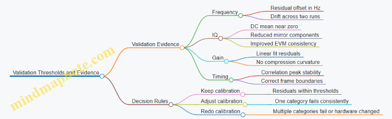
Practical Recordkeeping Checklist with Metadata
- Write down the reference identity: generator model or beacon ID, and its nominal frequency.
- Record hardware settings: SDR sample rate, RF gain, LO frequency, and any analog filters.
- Capture environmental context: temperature if available, and note when the measurement was taken.
- Save calibration outputs: coefficients, offsets, and correction factors with a clear naming convention.
- Confirm provenance: ensure the receiver uses the intended calibration file for the current band and gain range.
Example: A calibration file created for 2.4 GHz at RF gain 30 is accidentally applied at RF gain 40. The constellation looks “almost right” but EVM worsens. The fix is not another IQ tweak; it is using the correct gain-specific calibration set.
Troubleshooting Checklist When Reference Results Look Wrong
- If frequency is off but stable: correct LO programming or baseband frequency offset.
- If frequency jumps: check for retunes, buffer resets, or unstable generator settings.
- If IQ looks asymmetric: revisit DC removal order and confirm that the pilot is within the calibrated bandwidth.
- If gain is nonlinear: reduce RF gain, avoid compression, and redo the gain fit.
- If timing drifts: verify resampling settings and confirm the same burst length and correlation parameters.
A good calibration checklist ends with evidence you can point to: residual frequency error, constellation symmetry, linear gain behavior, and stable correlation peaks. When those four agree, the rest of the receiver chain usually behaves as designed.
6. Beam Tracking and Antenna Pointing Control Engineering
6.1 Coordinate Frames Az El and Earth Centered Inertial Transformations
A satellite ground station needs two coordinate views of the same pointing problem. The first is local to the antenna: azimuth and elevation (Az El). The second is global and inertial: Earth-Centered Inertial (ECI). Transformations between them let you compute where to point the antenna from an orbit solution, and then convert measured pointing back into a consistent reference.
What Each Frame Means
Az El is defined in the station’s local topocentric frame. Azimuth is measured in the horizontal plane from a reference direction (commonly true north, sometimes magnetic north depending on the system). Elevation is the angle above the local horizon. This frame is ideal for antenna control because servos naturally track angles.
ECI is a global Cartesian frame centered at Earth’s center. It is “inertial” in the sense that its axes do not rotate with Earth. Orbit propagators often output position and velocity in ECI (or a closely related inertial frame), making ECI a convenient starting point.
The key idea: you do not transform “the antenna.” You transform the satellite position vector from ECI into a local topocentric frame, then compute Az El from that local line-of-sight.
The Transformation Pipeline
A systematic pipeline avoids sign mistakes and unit confusion.
- Start with satellite state in ECI: position \(\mathbf{r}_{ECI}\) in meters.
- Convert ECI to Earth-fixed coordinates: ECI rotates with respect to Earth-fixed frames. Use Earth rotation angle (often via sidereal time) to compute \(\mathbf{r}_{ECEF}\).
- Compute the station position in Earth-fixed coordinates: from latitude, longitude, and altitude, obtain \(\mathbf{r}_{site,ECEF}\).
- Form the line-of-sight vector in Earth-fixed coordinates: \(\mathbf{\rho}*{ECEF}=\mathbf{r}*{ECI,to,ECEF}-\mathbf{r}_{site,ECEF}\).
- Rotate into the local topocentric frame: produce \(\mathbf{\rho}_{topo}=[x_{topo},y_{topo},z_{topo}]\) where axes align with east, north, and up.
- Compute elevation and azimuth: elevation comes from the up component; azimuth comes from the east and north components using \(\text{atan2}\).
This pipeline keeps the math grounded: Earth rotation is handled once, then local geometry is handled with a clear local rotation.
Mind Map: Frames and Transform Steps
Concrete Example: From ECI to Az El
Assume you have a propagated satellite position in ECI at a given epoch: \(\mathbf{r}_{ECI}=[X,Y,Z]\) meters. You also know the station geodetic coordinates: latitude \(\phi\), longitude \(\lambda\), altitude \(h\).
- Earth rotation: compute the rotation angle \(\theta\) that maps ECI to ECEF at that epoch. Apply a rotation about Earth’s spin axis to get \(\mathbf{r}_{ECEF}\).
- Station ECEF: compute \(\mathbf{r}_{site,ECEF}\) using the ellipsoid model so that the station sits on the correct surface.
- Line-of-sight: \(\mathbf{\rho}*{ECEF}=\mathbf{r}*{ECEF}-\mathbf{r}_{site,ECEF}\).
- Local rotation: rotate \(\mathbf{\rho}*{ECEF}\) into topocentric coordinates where \(z*{topo}\) is “up.”
- Elevation: \(\text{el}=\arcsin\left(\frac{z_{topo}}{|\mathbf{\rho}_{topo}|}\right)\).
- Azimuth: \(\text{az}=\text{atan2}(x_{topo},y_{topo})\) if \(x_{topo}\) is east and \(y_{topo}\) is north. The \(\text{atan2}\) argument order matters; swapping it mirrors azimuth.
If your system reports azimuth from north toward east, the above convention matches that behavior. If your system uses a different reference (for example, azimuth from south), you adjust the final azimuth by a fixed offset.
Practical Checks That Prevent “It Points Somewhere”
- Elevation sanity: if the satellite is below the horizon, elevation should be negative. If it is always positive, your “up” axis sign is likely flipped.
- Azimuth continuity: as the satellite passes through the sky, azimuth should change smoothly. Sudden jumps by ~180° usually indicate a wrong \(\text{atan2}\) argument order or a swapped north/east axis.
- Unit discipline: keep angles in radians inside trig functions and convert to degrees only at the interface to the antenna controller.
Advanced Detail: Why ECI to ECEF Matters
ECI is inertial, but the station is fixed to Earth. Without the ECI-to-ECEF step, you would effectively assume the station rotates with the inertial frame, which it does not. That mismatch produces systematic pointing errors that grow with time and with the satellite’s apparent motion.
A good engineering habit is to treat each rotation as a named, testable step. If you can verify intermediate vectors—like \(\mathbf{\rho}_{ECEF}\) magnitude staying consistent with geometry—you can isolate whether the error is in Earth rotation, station coordinate conversion, or the local topocentric rotation.
Example: Azimuth Reference Alignment
Suppose your computed azimuth \(\text{az}_{true}\) is measured from true north toward east. Your antenna controller expects azimuth from north toward east but uses a different internal convention for “north” (for example, it uses a local grid north approximation). In that case, you apply a small offset \(\Delta\text{az}\) derived from the difference between the controller’s reference and true north, then wrap the result into \([0,360)\). This keeps the transformation math intact while handling the local reference definition cleanly.
6.2 Tracking Algorithms for Continuous Pointing Under Motion
Continuous pointing means the antenna keeps a target in its beam while the spacecraft, Earth rotation, and mechanical motion all change the geometry. The core job of tracking algorithms is to turn time-varying geometry into smooth, accurate commands for azimuth and elevation (or other axes), while keeping the control loop stable and the RF link happy.
Foundational Model from Geometry to Commands
Start with a clear separation of responsibilities:
- Ephemeris and coordinate transforms produce the target line-of-sight direction in a chosen frame.
- Projection into antenna angles converts that direction into azimuth and elevation.
- Motion model and constraints account for servo limits, backlash, rate limits, and encoder wrap.
- Tracking filter and controller produce commands that are smooth enough for the mechanics but responsive enough for the link.
A practical workflow uses time-stamped inputs. For each control cycle at time \(t_k\), compute the desired pointing \((az_d, el_d)\) from the latest spacecraft state and site coordinates. Then compute the commanded motion \((az_c, el_c)\) after filtering and constraint handling.
Continuous-Time Tracking as a Discrete Loop
In a ground station, you typically run a loop at a fixed rate (for example, 50–200 Hz). The algorithm uses discrete updates:
- Predict target angles for the next cycle using the current angular rates (or by differencing recent angle estimates).
- Filter the desired angles to reduce jitter from ephemeris noise and measurement quantization.
- Command the servo with rate and acceleration limits.
- Correct using feedback from encoders and, if available, beacon-based pointing error.
A simple but effective prediction step is constant-rate extrapolation: \(az_{pred}=az_d + \dot{az}*d,\Delta t\), \(el*{pred}=el_d + \dot{el}_d,\Delta t\). If you don’t have \(\dot{az}_d\) and \(\dot{el}_d\), estimate them from the last two desired angle samples, then smooth the rates with a short moving average.
Angle Unwrapping and Frame Hygiene
Azimuth wrap is where many “it works on the bench” systems misbehave. Encoders often report angles modulo 360°, while control math needs continuity. Use unwrapping so the error \(e_{az}=az_{pred}-az_{meas}\) stays small even when crossing 0°/360°.
Also keep frames consistent. If your transforms output a direction vector, convert to angles once, near the end of the chain. Repeated conversions between frames can introduce small numerical noise that shows up as pointing jitter.
Filtering Desired Angles Without Lag Surprises
Filtering is not just “make it smooth.” It must preserve the true motion so the beam doesn’t lag behind the target. A common approach is a two-stage filter:
- Low-pass on angle increments: filter \(\Delta az\) and \(\Delta el\) rather than absolute angles.
- Rate limiting: enforce maximum command rates that match servo capability.
Example: Suppose the computed \(el_d\) has occasional 0.05° spikes from ephemeris quantization. If you low-pass absolute \(el_d\) too aggressively, the filter will smear those spikes into a slow drift. Filtering increments keeps the drift bounded because the command rate is constrained.
Constraint Handling for Real Mechanics
Servo constraints include:
- Maximum slew rate (deg/s)
- Maximum acceleration (deg/s²)
- Soft limits near mechanical stops
- Backlash and stiction
A robust command generator uses a “feasible trajectory” step. Compute the desired change \(\Delta az\) and \(\Delta el\), then clamp it so the implied rate and acceleration stay within limits. For backlash, a practical method is to apply a small deadband compensation: if the direction of motion reverses, add a short corrective bias until encoder feedback confirms motion.
Feedback Correction with Encoder and Beacon Error
Encoders provide measured angles \((az_{meas}, el_{meas})\). Use them to close the loop:
- Compute pointing error \(e_{az}=az_{cmd}-az_{meas}\), \(e_{el}=el_{cmd}-el_{meas}\).
- Apply a controller (often PID or PID with feedforward).
Feedforward matters because the target is moving even when the servo is perfect. Use predicted rates \(\dot{az}*{pred}\), \(\dot{el}*{pred}\) as feedforward terms, then let feedback correct residual errors.
If you have beacon-based pointing error (for example, from a received signal strength gradient or a dedicated tracking receiver), incorporate it as a slow correction layer. Keep it slower than the mechanical loop so you don’t fight the servo with noisy RF-derived estimates.
Mind Map: Continuous Pointing Under Motion
Example: Two-Axis Tracking with Rate Prediction and Clamping
Assume control cycle \(\Delta t=0.02\) s. At \(t_k\), you compute \(az_d=120.00°\), \(el_d=35.20°\). From recent samples, \(\dot{az}_d=0.80\) deg/s and \(\dot{el}_d=-0.30\) deg/s.
- Predict: \(az_{pred}=120.00 + 0.80\times0.02=120.016°\), \(el_{pred}=35.20-0.30\times0.02=35.194°\).
- Unwrap: ensure \(az_{pred}-az_{meas}\) is within ±180°.
- Filter increments: if \(el_d\) had a spike last cycle, filter \(\Delta el\) so the command changes smoothly.
- Clamp rates: if the servo max slew is 2 deg/s, the maximum angle change per cycle is \(2\times0.02=0.04°\). If the computed \(\Delta el\) would exceed that, clamp it.
- Command and feedback: set \(az_{cmd}, el_{cmd}\) to the clamped feasible values, then let the controller drive the error to near zero using encoder feedback.
Example: Handling Azimuth Wrap at 359° To 0°
Suppose \(az_{meas}=359.8°\) and the next predicted \(az_{pred}=0.2°\). Naively, the error is \(0.2-359.8=-359.6°\), which is nonsense for a small motion. After unwrapping, treat \(0.2°\) as \(360.2°\) for error computation, giving \(e_{az}=360.2-359.8=0.4°\). The servo then moves the short way, and the control loop stays well-behaved.
Practical Checklist for Stable Continuous Pointing
- Verify angle unwrapping on every update.
- Filter increments, not just absolute angles, to avoid lag drift.
- Enforce rate and acceleration limits before sending commands.
- Use feedforward from predicted rates and feedback from encoders.
- If beacon correction exists, apply it as a slow layer to avoid fighting the mechanical loop.
6.3 Servo Control Loop Tuning for Slew Rate and Settling Performance
A beam-tracking antenna behaves like a control system with a moving plant: motors, gears, bearings, and the antenna structure. Tuning is about choosing how aggressively the controller commands motion (slew rate) while keeping overshoot and oscillation low (settling). The key is to tune with the right measurement signals and to separate “fast motion” behavior from “final positioning” behavior.
Foundational Model of What You Are Tuning
Start by identifying the loop signals you can measure reliably:
- Commanded position from the tracking algorithm.
- Measured position from encoders or resolvers.
- Velocity estimate from differentiating position or using a tachometer.
- Motor drive feedback if available.
Then decide what you want the loop to do in two regimes:
- Slew regime: large position error, where you care about reaching the target quickly without hitting mechanical limits.
- Settle regime: small error near the target, where you care about minimizing overshoot and reducing residual jitter.
A practical mental model is a second-order system with damping. If damping is too low, you get ringing. If it’s too high, you get sluggish settling. Your tuning choices adjust that damping and the effective bandwidth.
Mind Map: Tuning Workflow and Design Choices
Step 1: Verify Scaling, Sign, and Units
Before touching gains, confirm that the loop is physically consistent. A common failure mode is a sign inversion between command and feedback, which turns a stabilizing loop into a self-excited one. Check that a positive command produces a positive measured motion in both axes. Also verify encoder counts to degrees or radians, and ensure velocity estimates have the correct units.
A simple test is to command a small step and observe the response with conservative drive limits. You should see motion in the expected direction and a smooth decay toward the target.
Step 2: Tune the Velocity Loop for Damping
If your system has a cascaded structure, tune the velocity loop first. Velocity feedback makes the system less sensitive to structural flex because it directly damps motion. Increase velocity-loop proportional gain until the response becomes quick but not oscillatory.
Use a step in position command that produces a moderate velocity demand. Watch for:
- Overshoot in position after the velocity settles.
- High-frequency oscillation that suggests noise amplification or resonance excitation.
If you add derivative action, keep it tied to measured velocity rather than raw differentiated position. Derivative on noisy signals can turn encoder quantization into a jitter generator.
Step 3: Tune the Position Loop for Settling
With the velocity loop stable, tune the position loop. Increase position proportional gain to reduce steady error and improve responsiveness, but stop before overshoot grows. A good practical target is a response that reaches the neighborhood of the setpoint quickly and then decays without sustained oscillation.
If you see ringing, reduce position proportional gain or increase damping via velocity feedback. If you see slow settling with minimal overshoot, you likely need more position gain or a carefully chosen integral term.
Step 4: Add Integral Only When You Need It
Integral action removes steady-state error caused by friction, gravity components, or small model mismatches. But integral can also reduce phase margin and cause slow oscillations.
A safe approach is to start with a very small integral gain and observe long-duration behavior during a tracking pass. If the antenna holds a constant offset under load, integral helps. If the system begins to “hunt” around the target, reduce integral or increase damping.
Step 5: Use Feedforward for Slew Rate Without Overdriving
Feedforward improves slew performance because it commands expected motion rather than waiting for the feedback loop to catch up. For tracking, feedforward can be based on predicted angular rate from the pointing solution.
A simple example: if the tracking algorithm predicts an angular velocity of 0.5 deg/s for a short interval, add a velocity feedforward term scaled to motor command units. Then let the feedback loop correct residual errors. This reduces the chance that the feedback loop saturates the drive during fast slews.
Example: Tuning a Two-Axis Antenna with Conservative Limits
Assume you have a cascaded controller with position PID and a velocity PI. You also have drive saturation limits.
- Set drive limits to 60% of normal and command a 1-degree step.
- Tune velocity loop: raise velocity proportional gain until the velocity reaches the demanded value quickly, then back off slightly to avoid oscillation.
- Tune position loop: increase position proportional gain until position overshoot is small and settling is acceptable.
- Add integral: increase integral gain until steady-state error is near zero, then stop before slow hunting appears.
- Validate slew: command a larger step that mimics real tracking rates and confirm the loop does not saturate for long.
If the larger step causes saturation, reduce position gain or add more feedforward so the controller does less work during the transient.
Performance Checks That Actually Matter
Measure these during tests:
- Settling time: time to remain within a small error band around the target.
- Overshoot: peak error beyond the target, which can translate into pointing loss.
- Residual oscillation: oscillation amplitude after settling, which can modulate received signal quality.
- Saturation duration: how long the drive stays at limits during slews.
When you tune, change one parameter at a time and record the response. That discipline prevents the classic “it got worse, but we changed five things” problem.
6.4 Antenna Model Effects Feed Horn Patterns and Polarization Alignment
Antenna models connect what you think the RF chain is doing to what the sky actually delivers. In practice, the feed horn pattern and polarization alignment determine the received power distribution across angle, the cross-polar leakage level, and the effective signal-to-noise ratio after beamforming and demodulation.
Feed Horn Patterns from Geometry to Field Strength
Start with the idea that a feed horn does not “illuminate” the reflector uniformly. Its radiation pattern is shaped by aperture size, flare angle, phase center location, and how the horn transitions to waveguide. In a ground station, you usually care about three pattern features:
- Main lobe width: sets how quickly gain drops as pointing error grows.
- Sidelobe levels: determine how much off-axis interference or Earth noise leaks into the receiver.
- Cross-polar discrimination: affects how much energy in the wrong polarization appears as usable signal.
A practical way to reason about the pattern is to treat it as a gain-versus-angle function, G(θ, φ), multiplied by a polarization response term. When you track a satellite, your pointing error changes with time, so the received carrier amplitude becomes time-varying even if the transmitter power is constant.
Polarization Alignment and Cross-Polar Leakage
Satellite signals arrive with a defined polarization basis, often linear or circular. Your receive chain has its own polarization basis set by the feed, orthomode transducer, and any polarization rotation in the mechanical or software pointing model.
If your receive polarization is rotated by an angle Δψ relative to the incoming polarization, the desired component scales roughly with cos²(Δψ), while the orthogonal component scales with sin²(Δψ). That orthogonal component is not just “lost”; it can also mix with the desired signal if the receiver processing assumes the wrong polarization.
Cross-polar leakage is commonly expressed as a ratio (often in dB). A useful engineering habit is to convert that ratio into an amplitude error estimate. For example, if cross-polar discrimination is 20 dB, the leaked orthogonal amplitude is about 10^(−20/20) = 0.1 of the desired amplitude, and the leaked power is about 1%.
Antenna Model Effects on Link Performance
An antenna model typically includes:
- Pointing geometry: where the beam points relative to the satellite line-of-sight.
- Pattern gain: G(θ, φ) from the feed and reflector combination.
- Polarization response: a mapping from incoming polarization to the receiver’s basis.
- Phase center and path length effects: which influence coherent processing and beam tracking.
Even if your SDR demodulator is perfect, a mismatch between the model and reality shows up as systematic SNR variation with elevation, azimuth, or polarization angle. That pattern is often repeatable, which is good news: it means you can measure it and correct your pointing and polarization calibration.
Mind Map: Feed Horn Patterns and Polarization Alignment
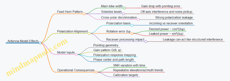
Example: Pointing Error Meets Pattern Gain
Assume the feed horn main lobe can be approximated near boresight by a Gaussian-like drop: G(Δθ) ≈ G0·exp(−(Δθ/σ)²). If σ corresponds to about 1.5° for a noticeable gain change, then a 0.75° pointing error reduces gain by exp(−(0.75/1.5)²) = exp(−0.25) ≈ 0.78, which is about −1.1 dB. That is large enough to matter for link margin, especially when tracking error grows near fast slews.
Example: Polarization Rotation Error in Linear Systems
Suppose the incoming signal is linearly polarized and your receive polarization is rotated by Δψ = 10°. Then the desired power factor is cos²(10°) ≈ 0.97 (about −0.13 dB), while the leaked orthogonal power is sin²(10°) ≈ 0.03 (about −15 dB relative to desired). If the orthogonal component contains interference or noise with different statistics, it can degrade demodulation even when the desired power loss looks small.
Example: Using Model Residuals to Tune Calibration
During a pass, record received carrier power versus time and compare it to the predicted power from your antenna model. If residuals correlate strongly with polarization angle but not with pointing error, the polarization alignment term is likely off. If residuals correlate with pointing error magnitude, the pattern gain or phase center model may need adjustment. The key is to separate geometry-driven effects from polarization-driven effects by checking which variable the residuals follow.
Practical Checklist for Engineering-Grade Modeling
- Verify the pattern gain is referenced to the same coordinate convention used by your tracking solution.
- Confirm polarization angle definitions match the feed’s physical orientation and any software sign conventions.
- Include cross-polar terms in the model when you expect significant polarization rotation or when the link is margin-sensitive.
- Treat phase center and path length consistently with your beam tracking timing and any coherent processing assumptions.
- Validate with measured beacon passes and look for repeatable residual structure rather than one-off anomalies.
6.5 Practical Pointing Verification Using Beacon Signals and Telemetry
Pointing verification is the step where you stop trusting the antenna model and start trusting what the sky (and your link) actually does. In practice, you combine beacon-based angle checks with telemetry-based sanity checks, then reconcile them into a single pointing error estimate.
Define What “Verified” Means
Start by choosing measurable outputs:
- Pointing error in angle: typically azimuth and elevation residuals in degrees or arcminutes.
- Polarization alignment indicator: cross-polar power ratio or demodulated quality metric.
- Time alignment: whether the antenna command time matches the RF observation time.
A simple acceptance rule helps. For example: “If the beacon-derived pointing residual stays within ±0.05° for 3 consecutive updates, the pointing loop is considered verified for that pass.” This prevents you from arguing about single noisy measurements.
Beacon Signal Strategy
Use beacons that are easy to detect and stable enough to measure angle. Common choices include:
- Continuous wave or narrowband carriers for robust carrier tracking.
- Known modulated beacons when you also need timing or demod quality.
Measure angle using one of these practical methods:
- Beam peak search around predicted pointing: step the antenna in small increments and find the maximum received power.
- Cross-track and in-track residual estimation: compare measured signal strength at two or more offsets to infer which direction the beam is missing.
- Polarization-based checks: if the beacon includes polarization information, use received polarization quality to confirm feed alignment.
A key detail: keep the step size consistent with your beamwidth. If your antenna 3 dB beamwidth is 1.0°, a step of 0.1° is usually small enough to map the peak without jumping past it.
Telemetry Sanity Checks Before You Trust the Beacon
Beacon measurements are only as good as the timestamps and coordinate frames. Before computing residuals, verify:
- Commanded vs measured antenna angles: compare commanded az/el to encoder-reported az/el.
- Servo mode and rate limits: confirm the antenna is in the expected tracking mode and not saturating.
- Time tags: ensure the beacon observation time corresponds to the encoder time, not the command issuance time.
A practical trick: compute residuals using the encoder angles at the moment your receiver reports the beacon metric. If you ignore this, you can “verify” pointing while actually verifying latency.
Compute Pointing Residuals from Beacon Metrics
Assume you have received power (or a demod quality metric) as a function of small az/el offsets. A systematic approach:
- Collect a small grid around predicted pointing, e.g., offsets of ±0.1° in az and el.
- Fit a local response surface. A simple quadratic fit around the peak is often enough.
- Extract the peak location and convert it to az/el residuals relative to predicted pointing.
If you only have one-dimensional scanning (say, elevation only), fit along that axis and treat az residual as “not verified” for that scan.
Integrated Mind Map
Mind Map: Practical Pointing Verification
Example Workflow with Concrete Numbers
Suppose predicted pointing is az=120.00°, el=35.00°. Your beacon metric is received carrier power after AGC settles.
- Telemetry pre-check: encoder reports az=120.02°, el=34.98° at the observation time, and servo mode is “track.” No saturation flags.
- Scan plan: step el by ±0.1° while holding az fixed. Use offsets: 34.90°, 35.00°, 35.10°.
- Measured metrics (relative power):
- el=34.90°: -18 dB
- el=35.00°: -6 dB
- el=35.10°: -10 dB
- Fit and peak: the peak lies near el=35.01°.
- Residual: elevation residual = 35.01° − 35.00° = +0.01°.
Now compare with telemetry residual between commanded and encoder. If commanded el was 35.00° but encoder at observation time was 34.98°, you have a 0.02° discrepancy that likely comes from latency or servo lag, not from the antenna model.
Diagnostic Reconciliation Rules
When beacon residual and telemetry residual disagree, you need a consistent interpretation:
- Beacon peak shifts but encoder matches command: likely coordinate transform or model error.
- Encoder lags behind command but beacon peak follows encoder: likely servo dynamics or control tuning.
- Beacon metric fluctuates without a clear peak: likely timing mismatch, AGC settling issues, or interference.
A good verification report includes the residual time series and a short diagnostic flag for the dominant error source, so the next pass starts with fewer guesses and more measurements.
7. Demodulation Signal Processing for Modulation Schemes
7.1 Carrier Recovery Techniques for Coherent and Noncoherent Modes
Carrier recovery estimates and removes the carrier’s frequency and phase so the demodulator sees a stable reference. In satellite links, the carrier is rarely perfect: Doppler shifts move the frequency, oscillators add phase noise, and mixers introduce offsets. The key split is whether the receiver preserves a known phase relationship to the transmitted carrier (coherent) or only needs energy and timing (noncoherent).
Coherent Mode Foundations
Coherent demodulation assumes the receiver can track the carrier phase well enough that constellation points rotate slowly. Practically, coherent receivers estimate a complex carrier term and rotate the incoming IQ samples by the negative of that estimate.
A simple mental model: if the received baseband is
- I/Q samples contain a term like
exp(j(2πΔf t + φ(t))) - where
Δfis residual frequency error andφ(t)is time-varying phase
Carrier recovery produces an estimate exp(-j(2π f̂ t + φ̂(t))) so the residual rotation becomes small.
Two common coherent strategies are frequency-then-phase tracking and joint tracking. Frequency-then-phase is often easier to debug: first remove most of the Doppler, then lock phase.
Noncoherent Mode Foundations
Noncoherent demodulation avoids needing an absolute carrier phase. Instead, it uses differential encoding, envelope detection, or energy-based metrics that are insensitive to unknown phase. This is useful when phase tracking is unreliable or when the modulation format does not require phase.
A useful rule of thumb: if the decision metric depends only on magnitude or on phase differences between consecutive symbols, then the receiver can tolerate larger phase uncertainty.
Mind Map: Carrier Recovery in Coherent and Noncoherent Modes
Coherent Acquisition Frequency Estimation
Coherent receivers typically start with a coarse frequency estimate. A practical approach uses a known preamble or pilot: correlate the received IQ with a locally generated reference over a grid of candidate frequencies. The grid step should be fine enough that the remaining frequency error does not smear symbols during the acquisition window.
Example: suppose your symbol duration is 1 ms and you can tolerate at most 10% of a cycle of residual rotation across one symbol. That implies a residual frequency error magnitude under about 100 Hz. If your Doppler uncertainty is ±20 kHz, you need a coarse search grid that can narrow the estimate to within that tolerance.
Coherent Phase Tracking with PLL or Costas Loop
After coarse frequency removal, phase tracking handles the remaining time-varying phase. A PLL (phase-locked loop) uses a phase detector and a loop filter to drive a numerically controlled oscillator (NCO). A Costas loop is a specialized PLL for suppressed-carrier signals, often used for BPSK/QPSK-like structures.
The loop bandwidth is the main design knob. Too narrow: the loop cannot follow phase noise and Doppler residuals, causing constellation rotation. Too wide: the loop chases noise, increasing decision errors.
A concrete tuning workflow:
- Start with a bandwidth that is small compared to the symbol rate so the loop does not react to symbol-to-symbol noise.
- Increase bandwidth if you see systematic rotation drift across the preamble.
- Decrease bandwidth if the constellation looks jittery even when frequency is correct.
Coherent IQ Rotation and Decision Feedback
Once you have an estimated carrier term, you rotate the IQ samples: I' + jQ' = (I + jQ) * exp(-jθ̂). For QPSK, this stabilizes the constellation so symbol decisions map cleanly to Gray-coded points.
If you still see errors clustered around specific constellation regions, check for IQ imbalance and DC offset. Carrier recovery can only correct phase and frequency; it cannot fix amplitude mismatch between I and Q.
Noncoherent Detection Strategies
Noncoherent receivers avoid absolute phase by changing the decision metric.
Differential detection works by encoding information in phase changes between consecutive symbols. If the transmitted symbol sequence is differentially encoded, the receiver estimates the phase difference rather than the absolute phase. This makes the receiver insensitive to constant phase offsets.
Example: with differential BPSK, the decision compares the sign of the real part of the product of the current and previous demodulated symbols. If the previous symbol is rotated by an unknown phase, that phase cancels in the product.
Envelope detection uses magnitude information. For amplitude-based modulations, the receiver tracks the envelope and compares it to thresholds. This can be robust to phase noise but is sensitive to amplitude fading and AGC behavior.
Noncoherent FSK metrics compare energy in frequency bins corresponding to candidate tones. Since the metric depends on power, unknown phase does not directly harm detection.
Shared Practical Example: Choosing Coherent or Noncoherent
Imagine two receivers processing the same downlink IQ recording.
- Receiver A uses coherent QPSK demodulation with a Costas loop. It performs well when SNR is moderate and the loop bandwidth is tuned so the constellation stops rotating.
- Receiver B uses differential detection. It tolerates larger phase uncertainty, but errors can increase when timing is off because the phase difference estimate becomes inconsistent.
Both approaches can be correct; the difference is whether you spend effort on phase tracking or on choosing a phase-insensitive decision rule.
Summary of the Integrated Workflow
Coherent mode typically follows: coarse frequency acquisition → phase tracking with a loop → IQ rotation → symbol decisions, with calibration checks for IQ imbalance. Noncoherent mode typically follows: timing alignment → compute a phase-insensitive metric (differential, envelope, or energy) → decide symbols without requiring absolute carrier phase. In both cases, the receiver’s success hinges on matching the carrier recovery method to the modulation structure and the quality of the IQ stream.
7.2 Symbol Timing Recovery Matched Filtering And Resampling
Symbol timing recovery answers a simple question: where, exactly, should you sample the received waveform so each symbol’s energy lands in the right place? In practice, you combine three ideas: matched filtering to maximize signal-to-noise ratio, timing estimation to learn the sampling phase, and resampling to produce a steady stream of symbol-spaced samples.
Matched Filtering for the Best Sampling Instants
Matched filtering uses a filter shaped like the expected transmitted pulse. If the transmitted baseband pulse is \(p(t)\), the matched filter is proportional to \(p^*(-t)\). The output peaks when the sampling time aligns with the symbol center, and the peak-to-noise ratio is maximized under standard assumptions.
A concrete example: suppose your modulation uses root-raised cosine (RRC) pulses with roll-off \(\beta=0.25\) and a symbol rate \(R_s\). You implement an RRC matched filter at the receiver. If you sample at the correct timing, the filter output for a single isolated symbol resembles a main lobe with controlled sidelobes; if you sample early or late, the main lobe energy spreads into adjacent symbol decisions.
Matched filtering also sets up a useful reality: after the matched filter, the overall impulse response is approximately the raised-cosine (for ideal transmit/receive pulse pairing). That means timing errors show up clearly as inter-symbol interference (ISI) patterns.
Timing Error Signals from Filtered Waveforms
Once you have the matched-filtered signal, you estimate the timing offset \(\tau\) between the receiver’s sampling grid and the true symbol centers. A common approach uses a timing error detector that compares early and late samples.
A practical early-late gate method:
- Pick a fractional timing offset \(\Delta\) (often a small fraction of the symbol period).
- Compute two samples around the current estimate: \(y(t+\Delta)\) and \(y(t-\Delta)\).
- Form an error proportional to the difference in their magnitudes or energies.
Intuition: when you are early, the “late” sample tends to be closer to the peak, so the error pushes the estimate toward later sampling. When you are late, the opposite happens. The error detector output drives a loop that updates \(\tau\).
Resampling to Produce Symbol Spaced Samples
After timing recovery, you still need to convert the continuous-time (or high-rate discrete-time) matched-filter output into symbol-spaced samples. Resampling performs interpolation at the estimated fractional delay.
A straightforward method uses a fractional delay filter. If your matched-filter output is sampled at \(F_s\) and you want one sample per symbol, the resampler maps input indices to output indices using \(\tau\). The key is that interpolation must preserve the pulse shape enough that the decision device sees near-ideal symbol timing.
Example workflow:
- Matched filter the IQ stream.
- Run a timing loop to estimate \(\tau\) each update.
- Use \(\tau\) to interpolate the next symbol sample from the surrounding matched-filter samples.
- Feed the resulting symbol stream to the demodulator.
Mind Map: Symbol Timing Recovery with Matched Filtering and Resampling
Example: Early-Late Gate with a Simple Loop
Consider a receiver where the matched-filter output is available at \(F_s\) samples per second, and the symbol period is \(T_s\). Maintain a timing estimate \(\tau_k\) and update it each symbol.
- For the current estimate, compute early and late samples:
- \(e_k = y(n_k - \Delta_n)\)
- \(l_k = y(n_k + \Delta_n)\) where \(n_k\) is the nearest integer index to the desired sampling instant and \(\Delta_n\) corresponds to \(\Delta\) in samples.
- Form an error:
- \(\epsilon_k = |l_k|^2 - |e_k|^2\)
- Update the timing estimate:
- \(\tau_{k+1} = \tau_k + \mu,\epsilon_k\)
The step size \(\mu\) controls loop speed and stability. If \(\mu\) is too large, the estimate jitters and the resampler produces wandering sample phases. If \(\mu\) is too small, lock takes longer and the demodulator sees extra ISI during acquisition.
Example: What You See When Timing Is Wrong
If you skip timing recovery and sample on a fixed grid, the matched-filter output will not align with the pulse peaks. For RRC-shaped signals, this misalignment turns the intended near-zero ISI into significant adjacent-symbol contributions. In a constellation plot, you may still see a recognizable pattern, but decision boundaries become unreliable because the symbol stream is effectively “smeared” by timing error.
With timing recovery enabled, the resampler places samples at the peak of the matched-filter response, and the ISI terms shrink. The constellation tightens because the demodulator receives samples that correspond more closely to the intended symbol instants.
Practical Implementation Notes That Prevent Common Bugs
- Use the matched filter before timing estimation; estimating timing on unfiltered noise makes the error detector erratic.
- Keep the early-late spacing small enough to approximate a local slope, but large enough to produce a measurable error.
- Ensure the resampler uses the same timing estimate that the loop updates; mismatched timing paths create a “double error.”
- Validate by checking that the symbol-spaced stream shows reduced ISI compared to a fixed-grid sampler.
When these pieces work together, timing recovery becomes less of a mystery and more of a disciplined pipeline: filter for a clean peak, estimate the fractional offset from local comparisons, and resample so the demodulator gets what it expects.
7.3 QPSK BPSK and OQPSK Demodulation With SDR Implementations
Demodulation turns received IQ samples into bits, but the “how” depends on the modulation’s geometry and timing. With SDR, you typically run a pipeline: front-end conditioning, carrier recovery, timing recovery, symbol decisions, and finally bit mapping. The key is to keep each stage’s assumptions consistent with the modulation format, or you’ll get confident-looking wrong answers.
Foundational Signal Model and Decision Targets
For BPSK, each symbol carries one bit and maps to a phase of either 0 or π relative to the recovered carrier. For QPSK, two bits share one symbol, mapped to four phases (often Gray-coded). For OQPSK, the I and Q components are offset by half a symbol period to reduce abrupt phase changes.
In practice, after carrier and timing are aligned, you want one complex sample per symbol. Then:
- BPSK decision is based on the sign of the real component after rotation.
- QPSK decision is based on the signs of real and imaginary components.
- OQPSK decision is based on staggered I and Q decisions, then interleaving bits.
SDR Pipeline for Coherent Demodulation
A coherent receiver assumes you can estimate and remove the carrier’s frequency and phase. That means you rotate the incoming IQ by the negative of the estimated carrier phase, so constellation points land where your decision logic expects them.
A systematic SDR pipeline looks like this:
- Resample and filter to match the symbol rate and reduce out-of-band noise.
- Carrier recovery to estimate frequency offset and phase.
- Timing recovery to choose the correct sampling instant per symbol.
- Matched filtering or equivalent pulse shaping compensation.
- Symbol-to-bit mapping using the modulation’s constellation rules.
A practical example: if your symbol rate is 1 Msps and your SDR provides 10 Msps, you resample to 2 Msps or 1 Msps depending on your processing budget, then use a root-raised-cosine matched filter so the eye diagram behaves.
BPSK Demodulation with SDR
After carrier rotation, BPSK symbols cluster around +1 and −1 on the real axis. A simple decision rule is:
- If Re{z} ≥ 0 → bit 1 (or 0, depending on your mapping)
- Else → the opposite bit
Example practice: Suppose your transmitter maps bit 0 to phase 0 and bit 1 to phase π. After rotation, you expect bit 0 near +1 and bit 1 near −1. If your bit error rate is high but the constellation looks rotated, the issue is usually carrier phase ambiguity, not the decision rule.
QPSK Demodulation with SDR
QPSK uses four phases, so you need both I and Q decisions. After rotation, a common Gray mapping uses:
- Re{z} sign gives one bit
- Im{z} sign gives the other bit
Example practice: If you use Gray mapping where (I,Q) = (+,+) → 00, (+,−) → 01, (−,+) → 11, (−,−) → 10, then your bit extraction is just sign checks plus a lookup table.
Timing matters: if you sample half a symbol late, the constellation smears and the sign decisions become noisy. That’s why timing recovery should happen before hard decisions.
OQPSK Demodulation with SDR
OQPSK offsets Q relative to I by half a symbol period. That means you cannot treat I and Q as arriving at the same instant. A clean approach is:
- Recover carrier phase and rotate IQ.
- Perform timing recovery to establish the symbol grid.
- Sample I at symbol boundaries and Q at half-boundaries.
- Decide I bits from I samples and Q bits from Q samples.
- Interleave bits to reconstruct the original stream.
Example practice: If your symbol period is T, then I samples occur at t = nT and Q samples at t = nT + T/2. In an SDR implementation, you can realize this by using two fractional-delay sampling points or by maintaining two timing offsets in your resampler.
Mind Map: Demodulation Pipeline and Modulation-Specific Decisions
Example: Minimal Decision Stage Pseudocode
The following pseudocode assumes you already have one complex symbol sample per decision time (and for OQPSK, you have separate I and Q sampling instants).
# Inputs: ZI, ZQ Are Complex Samples After Carrier Rotation
# For BPSK: z is complex symbol sample
# For QPSK: Z Is Complex Symbol Sample
# For OQPSK: zI and zQ correspond to staggered sampling times

# BPSK
bit_bpsk = (real(z) >= 0) ? 1 : 0

# QPSK with Gray-Style Sign Mapping
bI = (real(z) >= 0) ? 1 : 0
bQ = (imag(z) >= 0) ? 1 : 0
bits_qpsk = gray_lookup(bI, bQ)

# OQPSK
bitI = (real(zI) >= 0) ? 1 : 0
bitQ = (real(zQ) >= 0) ? 1 : 0
bits_oqpsk = interleave(bitI, bitQ)
Integrated Debugging Practices That Actually Help
When results are wrong, start with geometry: plot the constellation after carrier rotation and matched filtering. If BPSK points sit on the imaginary axis, your phase rotation is off by about 90 degrees. If QPSK points form a cross instead of four clusters, timing recovery is likely sampling between symbol centers. For OQPSK, if I and Q bits look like they belong to different symbol indices, your half-symbol offset is misapplied.
The demodulator is only as good as the assumptions you enforce: one sample per symbol for BPSK/QPSK, and staggered sampling for OQPSK. Once those are correct, the decision rules are straightforward—and that’s the point where SDR becomes pleasantly boring.
7.4 FSK and PSK Variants for Narrowband Receivers
Narrowband receivers often care more about frequency and phase stability than about wideband flexibility. That bias shapes everything: how you choose the modulation variant, how you build the demodulator, and how you set receiver parameters like bandwidth, loop bandwidth, and decision thresholds.
Core Idea: What Narrowband Receivers Optimize
Start with the signal model. In narrowband links, the occupied bandwidth is small compared to the RF carrier, so the receiver can treat the channel as mostly “one tone plus controlled variation.”
- FSK varies the instantaneous frequency between discrete values. The demodulator’s job is to measure frequency changes over short windows.
- PSK varies the carrier phase among discrete states. The demodulator’s job is to measure phase relative to a reference.
A practical rule: if your receiver can maintain a clean carrier reference, PSK variants usually give better spectral efficiency. If your reference is shaky but frequency measurement is reliable, FSK variants can be easier to make robust.
FSK Variants and Their Receiver Implications
FSK family members differ mainly in how many frequency states exist and how transitions are shaped.
2-FSK and Binary FSK
Binary FSK uses two frequencies, often written as f0 and f1. The receiver typically uses a frequency discriminator approach or a coherent frequency demodulator.
Example: Suppose the symbol rate is 1 ksym/s and the frequency separation is 200 Hz. A simple discriminator can integrate the phase slope over each symbol period. If your integration window is too short, noise dominates; too long, inter-symbol transitions smear.
Key parameter relationships:
- Frequency deviation controls how separated the discriminator outputs are.
- Symbol duration controls how much averaging you can do.
- Receiver front-end bandwidth must be wide enough to pass both tones but narrow enough to reject out-of-band interference.
M-FSK and Tone Bank Demodulation
For M-FSK, there are M possible tones. A common narrowband technique is a tone bank: mix down, then correlate or filter against each expected tone.
Example: With M=4, you can implement four narrow correlators centered at the expected offsets. The correlator with the largest magnitude wins. This is computationally heavier than 2-FSK, but it can be very stable when the channel is mostly stationary over a packet.
Tradeoff: tone spacing must exceed the effective noise bandwidth of each correlator, or decisions become ambiguous.
Gaussian Shaped FSK and Bandwidth Control
Some systems use shaped frequency transitions to reduce spectral splatter. The receiver still measures frequency, but the discriminator output becomes smoother.
Example: If you use a discriminator that assumes abrupt transitions, shaped transitions can bias the decision near symbol boundaries. The fix is to align the decision timing with the expected transition shape, or to use a matched filter style approach.
PSK Variants and Their Receiver Implications
PSK family members differ in how many phase states exist and how the receiver handles phase ambiguity.
BPSK and Coherent Detection
BPSK uses two phases separated by 180 degrees. Coherent detection multiplies the received signal by a synchronized carrier reference, then integrates over the symbol.
Example: If your local oscillator has a small phase error that drifts slowly, the integrated decision statistic remains mostly correct. If the phase error jumps within a symbol, the decision can flip.
So the receiver needs:
- A carrier recovery loop with enough bandwidth to track drift.
- A symbol timing strategy that avoids integrating across transitions.
QPSK and Quadrature Decision
QPSK uses four phases. After carrier recovery, you can separate decisions into two quadrature components.
Example: If the constellation rotates due to residual phase error, both I and Q decision boundaries shift together. A practical mitigation is to use a decision-directed phase correction step after initial acquisition.
Differential PSK for Noncoherent Convenience
Differential PSK encodes information in the phase change between consecutive symbols rather than absolute phase.
Example: If the receiver cannot maintain a stable carrier reference, differential detection compares the current symbol’s phase to the previous one. This avoids needing perfect phase synchronization, at the cost of extra sensitivity to noise because each decision depends on two symbols.
A simple way to see it: coherent PSK compares to a reference; differential PSK compares to yesterday’s decision. If yesterday was wrong, today inherits the error.
Mind Map: Narrowband FSK and PSK Receiver Design
Example Walkthrough: Choosing Between FSK and PSK
Assume you have a narrowband receiver with limited ability to lock a clean carrier reference. You also expect moderate frequency offsets.
- If frequency offsets dominate and phase tracking is unreliable, start with 2-FSK or a shaped FSK variant. Use a discriminator with an integration window matched to the symbol duration.
- If phase tracking is stable and you can maintain a reference, use BPSK or QPSK with coherent integration. Tune loop bandwidth so the phase error stays small within a symbol.
- If you cannot guarantee either, use differential PSK. Expect a performance hit, but gain operational simplicity.
Practical Decision Rules That Prevent Common Failure Modes
- Bandwidth mismatch: if the RF/IF bandwidth is too narrow, tones or phase trajectories get distorted; if too wide, noise and interferers raise decision errors.
- Integration window mismatch: too short wastes SNR; too long smears transitions.
- Loop bandwidth mismatch: a loop that is too slow lags drift; too fast chases noise.
When these rules are followed, FSK and PSK variants become predictable tools rather than mysterious black boxes.
7.5 Practical Demodulation Pipelines With Example Parameter Sets
A practical demodulation pipeline is less about one magic algorithm and more about a sequence of checks: frequency alignment, timing alignment, channel conditioning, then symbol decisions. Below is a systematic receive-to-bits flow that you can implement in an SDR chain, with example parameter sets that match common space-link realities like Doppler drift, residual IQ imbalance, and imperfect front-end filtering.
Mind Map: Demodulation Pipeline with Parameter Touchpoints
Step 1: Input IQ Conditioning
Start by making the IQ stream behave like a clean mathematical model. Remove DC offsets, correct IQ gain/phase imbalance if you have calibration, and apply AGC carefully so it doesn’t fight the signal dynamics.
Example parameter set (front-end conditioning):
- DC removal: enabled, update rate 1–5 kHz
- IQ imbalance correction: enabled if you have a calibration sweep
- AGC: target RMS 0.1–0.3 of full-scale, attack 1–5 ms, release 20–100 ms
- Optional: low-pass or band-pass to narrow the processing bandwidth to the expected occupied spectrum
Concrete check: after conditioning, the constellation should stop “breathing” in radius when the signal strength changes slowly.
Step 2: Frequency Alignment
Space links rarely sit still. Use a two-stage approach: coarse frequency search to land near the carrier, then fine tracking to follow residual offset and Doppler rate.
Example parameter set (coarse + fine):
- Coarse search range: ±50 kHz around predicted carrier
- Coarse step: 500 Hz to 2 kHz
- Coarse metric: peak of correlation with a known preamble or maximum of spectral energy in the expected subband
- Fine tracking loop bandwidth: 10–200 Hz for stable tracking
- Fine loop update rate: 1–10 kHz
Concrete check: if fine tracking repeatedly loses lock, reduce loop bandwidth or widen the coarse search range.
Step 3: Timing Alignment
Timing recovery is where many “it almost works” systems fail. Use matched filtering first, then estimate symbol timing, then apply fractional delay.
Example parameter set (timing recovery):
- Matched filter: root-raised cosine (RRC)
- RRC roll-off: 0.2–0.35
- Symbol timing estimator: Gardner or Mueller and Müller
- Timing loop bandwidth: 0.01–0.1 of symbol rate
- Fractional delay method: polyphase filter with 32–64 taps
Concrete check: after timing correction, the eye opening should be stable across multiple frames, not just one.
Step 4: Channel Conditioning
Even with good RF hardware, you’ll see residual phase noise, amplitude ripple, and multipath-like effects from reflections or polarization mismatch. Keep the equalizer simple and bounded.
Example parameter set (equalization and phase):
- Equalizer type: complex LMS or decision-directed LMS
- Tap count: 11–31 taps
- Step size (LMS): 1e-4 to 5e-3 depending on SNR
- Decision delay: 1–3 symbols
- Optional phase smoothing: 2nd-order PLL or moving average on phase error
Concrete check: equalizer taps should converge quickly during preamble, then stop thrashing during payload.
Step 5: Symbol Decisions and Soft Metrics
For coded links, soft decisions usually beat hard decisions. Produce log-likelihood ratios (LLRs) when you can, or at least soft symbol metrics.
Example parameter set (QPSK soft decisions):
- Constellation: Gray-coded QPSK
- Soft metric: LLR computed from Euclidean distance to nearest constellation points
- LLR scaling: normalize by estimated noise variance
- Noise variance estimate: from preamble residual error or from a sliding window of decision error
Concrete check: LLR magnitudes should be consistent across frames; if they collapse to near zero, your noise estimate is off or tracking is unstable.
Step 6: Frame Synchronization and Output Validation
Frame sync prevents you from “decoding noise politely.” Use a preamble correlator, then verify with CRC.
Example parameter set (frame sync):
- Correlator: complex correlation over preamble length
- Threshold: start at 6–10 dB above median correlation floor
- Peak-to-sidelobe requirement: enforce a minimum ratio to avoid false peaks
- CRC: enable and treat CRC failures as a diagnostic signal, not just a statistic
Concrete check: when CRC fails, inspect whether the failure correlates with frequency tracking loss, timing drift, or equalizer divergence.
Example End-to-End Parameter Set Summary
Use these as starting points, then tune based on observed lock behavior.
- Sample rate: 4× to 8× symbol rate
- RRC roll-off: 0.25
- Coarse frequency search: ±50 kHz, 1 kHz step
- Fine carrier loop bandwidth: 50 Hz
- Timing loop bandwidth: 0.03× symbol rate
- Equalizer taps: 21, LMS step 1e-3
- Soft decisions: LLR from distance metrics with noise variance from preamble
- Frame sync: preamble correlator with threshold and CRC gating
A good pipeline is one where each stage has a measurable “pass” condition: frequency lock metric peaks, timing error variance drops, equalizer error stabilizes, and CRC passes. When one stage fails, you know exactly where to look—no guessing, no mystery meat.
8. Channel Impairment Modeling and Receiver Robustness
8.1 Additive Noise Phase Noise and Nonlinear Distortion Effects
A satellite receiver is a chain of imperfect parts, and three effects often dominate what you see in baseband: additive noise, phase noise, and nonlinear distortion. Additive noise sets the floor. Phase noise smears the carrier and makes demodulation harder even when SNR looks decent. Nonlinear distortion creates new spectral components that can land right where your signal lives. The trick is to understand how each effect enters the chain and how it shows up in measurements.
Additive Noise Foundations and Where It Comes From
Additive noise in an RF receiver is usually modeled as a noise source added at some reference point, then carried through the rest of the chain. In practice, you can think of it as thermal noise from resistive elements plus excess noise from active devices.
Start with the simplest mental model: the receiver input sees a signal plus noise. After amplification, both signal and noise scale, but the noise figure tells you how much extra noise the receiver adds compared to an ideal amplifier. If you have a low-noise amplifier (LNA) early, you protect the later stages from having to amplify their own noise contributions.
A concrete example: suppose your antenna delivers a weak carrier at -120 dBm. If your LNA has a noise figure of 1 dB, the effective noise at the LNA output in a 1 Hz bandwidth is only about 1.26× the ideal thermal noise. If instead you place a higher-noise stage before the LNA, the same -120 dBm signal gets buried by the amplified noise from that first stage.
In SDR receivers, additive noise also includes quantization noise from the ADC. Quantization noise behaves like noise added after the analog chain, shaped by sampling rate and effective number of bits. If you set gain too low, quantization noise rises relative to the signal; if you set gain too high, nonlinear distortion rises and can be worse than quantization.
Phase Noise Mechanisms and Demodulation Impact
Phase noise is random fluctuation in the oscillator phase, which turns a pure tone into a carrier plus a skirt of noise around it. In a downconversion receiver, phase noise on the local oscillator (LO) becomes phase noise on the demodulated signal.
A useful way to reason is to separate two roles:
- Carrier smearing: the demodulator expects a stable phase relationship. Phase noise breaks that assumption.
- Interference within the signal band: the phase-noise skirt can overlap the modulation spectrum, effectively raising the noise floor in a frequency-dependent way.
Example: consider a BPSK or QPSK signal. If the LO has significant phase noise, the recovered carrier will jitter, and the constellation points will rotate and blur. Even if the measured wideband SNR looks acceptable, the bit error rate can worsen because the decision boundaries become less reliable.
In frequency planning, phase noise matters most when the LO offset places the phase-noise skirt near the signal’s occupied bandwidth. In direct sampling, LO phase noise still appears, but the mapping between offset frequency and demodulation impact changes with architecture.
Nonlinear Distortion Sources and Spectral Artifacts
Nonlinear distortion occurs when a device’s gain depends on input amplitude or when its transfer curve is not perfectly linear. The result is harmonic generation and intermodulation products. In satellite links, you often have a strong carrier plus weaker adjacent signals or spurs, so intermodulation can be the villain.
A practical model uses two ideas:
- Compression: as input power approaches the device’s 1 dB compression point, gain drops and distortion rises.
- Intermodulation: for two tones, the third-order intermodulation products often dominate near the carrier.
Example: imagine two signals at frequencies f1 and f2 entering a receiver. If the front-end is nonlinear, you can get components at 2f1−f2 and 2f2−f1. If one of those lands inside your desired signal band, it behaves like an interferer, not like random noise.
Nonlinear distortion also interacts with phase noise. A distorted waveform can produce additional phase modulation components, which can make the constellation look worse than expected from phase noise alone.
Integrated View of Effects in an SDR Receiver
To connect the three effects, track where they enter:
- Additive noise enters early and sets the baseline. It is mostly independent of signal amplitude.
- Phase noise enters through the LO and shows up as frequency-dependent degradation around the carrier.
- Nonlinear distortion enters when signal amplitude is high enough to push devices out of linear operation.
This is why gain staging is not just about maximizing SNR. It is about balancing noise floor, phase-noise visibility, and distortion products.
Mind Map: Noise, Phase Noise, and Nonlinear Distortion
Example Workflow for Diagnosing Which Effect Dominates
- Check gain and headroom: reduce RF gain until spurs and constellation “fuzz” decrease. If improvement is strong, nonlinear distortion was likely dominating.
- Inspect spectrum around the carrier: if the noise rises close to the carrier but not far away, phase noise is a prime suspect.
- Compare measured noise floor to expected: if the floor is higher than predicted from noise figure and bandwidth, additive noise sources or ADC quantization may be limiting.
A small, concrete scenario: you observe a constellation that looks worse when you increase input power by 10 dB. If the spectrum shows growing spurs and the noise floor rises unevenly, nonlinear distortion is likely. If the constellation worsens even at low input power and the spectrum shows a carrier skirt, phase noise is likely. If both remain stable with power but BER is still poor, additive noise is likely the limiter.
Practical Takeaways for Engineering Decisions
- Place the lowest-noise amplification as early as possible to minimize additive noise growth.
- Ensure LO quality and offset planning so the phase-noise skirt does not flood the modulation bandwidth.
- Keep the RF chain and ADC out of compression; treat intermodulation products as potential in-band interferers.
When you apply these rules together, you stop treating “noise” as one thing. You start treating it as a set of distinct mechanisms, each with its own signature and engineering lever.
8.2 Doppler Dynamics and Their Compensation in Baseband
What Doppler Does to Your Signal
Doppler shift is the frequency change caused by relative motion between satellite and ground station. In baseband processing, it shows up as a time-varying carrier offset that drifts across your receiver’s demodulator bandwidth. If you treat it as a constant, you may get away with it for short passes or narrow symbol rates, but longer passes and higher carrier frequencies usually punish that shortcut.
A useful starting point is the received carrier model:
- The instantaneous received frequency equals the transmitted carrier plus a Doppler term.
- The Doppler term changes with time because range rate changes with geometry.
In practice, you rarely know the exact Doppler curve, so you estimate it from the signal (or from ephemeris plus a correction loop) and then remove it in baseband.
From Geometry to Doppler Rate
Doppler is tied to line-of-sight velocity. As the satellite moves, the line-of-sight component of velocity changes, producing both a shift and a drift. The drift matters because demodulators often assume the carrier is stable over a symbol or frame.
A systematic way to reason about it:
- Compute or estimate line-of-sight velocity versus time.
- Convert it to Doppler frequency shift.
- Differentiate to get Doppler rate, which predicts how fast the offset moves.
For an engineering check, compare the expected Doppler rate to your receiver’s acquisition and tracking capabilities. If the offset moves faster than your loop can follow, you’ll see rising bit errors even when the average SNR looks fine.
Baseband Compensation Strategies
Baseband compensation usually combines three layers: coarse correction, tracking, and residual cleanup.
Coarse correction uses a predicted Doppler from ephemeris or a frequency estimate from a preamble. You mix the IQ samples by a complex exponential at the estimated offset.
Tracking refines the estimate continuously. Common approaches include:
- Frequency-locked loops that update a numerically controlled oscillator.
- Decision-directed carrier recovery for coherent modulations.
- Non-data-aided estimators for robustness when decisions are unreliable.
Residual cleanup handles the fact that Doppler is not perfectly modeled. You may apply a final frequency correction after frame sync, or let the carrier recovery loop absorb the remaining error.
Mind Map: Doppler Dynamics and Compensation
Example: Estimating and Removing Doppler in IQ Samples
Assume you have complex IQ samples centered near baseband but with a Doppler-induced carrier offset. You estimate a coarse carrier frequency offset (CFO) from a known preamble, then mix it out.
import numpy as np

fs = 2.0e6                 # sample rate in Hz
f_cfo = 1200.0             # estimated CFO in Hz
N = 4096

n = np.arange(N)
# Iq Is Complex64/complex128 Array of Length N
# iq[n] = I[n] + 1j*Q[n]

rot = np.exp(-1j * 2*np.pi * f_cfo * n / fs)
iq_corr = iq[:N] * rot
After coarse mixing, you still expect drift. That drift is what the tracking loop should handle. A good sanity check is to compute the residual frequency estimate over successive windows; if it trends smoothly, your loop bandwidth is likely appropriate.
Example: Choosing Tracking Loop Bandwidth with Doppler Rate
Suppose your Doppler rate is about 50 Hz per second during a pass segment. If your tracking loop bandwidth is too narrow, it will lag and leave a growing residual CFO.
A practical rule of thumb is to set the loop bandwidth so it can follow the drift within the loop’s effective time constant. For instance, if your loop time constant is 0.1 s, then the expected CFO change over that time is roughly 5 Hz. That’s small enough that the residual error stays within the demodulator’s tolerance.
If instead the time constant is 1 s, the CFO change is about 50 Hz, which often forces the demodulator to work harder than it should.
Practical Diagnostics That Prevent “Mystery” Failures
When Doppler compensation is wrong, symptoms are usually consistent:
- The constellation rotates steadily during a frame.
- Carrier recovery error does not settle.
- Frame sync works intermittently, then fails as the pass geometry changes.
To diagnose efficiently:
- Verify coarse CFO estimate quality using a short preamble window.
- Measure residual CFO trend across time windows.
- Confirm tracking loop bandwidth relative to estimated Doppler rate.
A receiver that “almost works” is often a loop tuning mismatch, not a mysterious RF problem. Doppler dynamics are predictable; your job is to make the baseband processing keep up.
8.3 Automatic Frequency and Timing Search Strategies
Automatic frequency and timing search is what lets a receiver start from “no idea” and still lock onto a real satellite signal. In practice, you’re searching for two things: the carrier frequency offset (CFO) and the symbol timing offset (STO). The receiver can’t demodulate until both are close enough for its tracking loops to behave.
Foundational Model of Offsets
Assume the received complex baseband signal is
- A carrier term with frequency error: \(e^{j2\pi \Delta f t}\)
- A timing shift: \(x(t-\tau)\)
- Plus noise and channel effects
CFO mainly rotates the constellation over time. Timing error mainly smears symbols and reduces the peak of correlation-based detectors. That separation is useful: frequency search can often be done on blocks where timing is roughly handled, and timing search can be done after a coarse CFO is removed.
Search Strategy Overview
A robust receiver typically uses a staged approach:
- Coarse frequency search using a method that tolerates unknown timing.
- Fine frequency refinement using a metric that improves when timing is closer.
- Coarse timing search using correlation or energy metrics.
- Fine timing refinement using decision-directed or pilot-assisted methods.
This order is common because frequency error causes rapid phase rotation that can confuse timing metrics. If you can reduce CFO first, timing search becomes cleaner.
Coarse Frequency Search Methods
FFT-Based Spectral Scan
If you have a block of IQ samples, you can estimate CFO by looking for where energy concentrates after mixing with candidate frequencies. A practical implementation uses an FFT of a windowed segment and finds the strongest bin near the expected center.
Example: Suppose your receiver expects a downconverted signal near 10.000 MHz, but the true CFO could be ±50 kHz due to oscillator drift and Doppler. You choose an FFT span of 200 kHz and compute the magnitude spectrum. The peak bin gives a coarse CFO estimate. You then mix the signal by the negative of that estimate.
Key practice: use a window (like Hann) to reduce sidelobes, and ensure the FFT bin spacing is fine enough that the peak is not “jumping” between bins due to noise.
Cyclic Prefix and Periodicity Metrics
For waveforms with known periodic structure, you can use metrics that peak when the frequency offset aligns with the periodicity. This can be more reliable than raw energy when interference is present.
Example: If your signal has a repeating preamble pattern, compute a correlation between the received block and delayed versions of itself. CFO changes the phase relationship between repeats, so the correlation magnitude peaks near the correct CFO.
Fine Frequency Refinement
After coarse CFO removal, you can refine using a phase-based estimator.
- Pilot-aided phase slope: If pilots are known, estimate the phase difference between consecutive pilot symbols and convert the slope to CFO.
- Cost function maximization: For preambles, evaluate a likelihood or correlation metric across a small CFO grid.
Example: After coarse search, you’re within ±200 Hz. You test CFO candidates spaced at 20 Hz over a 400 Hz range. For each candidate, you remove CFO, run a short correlation with the preamble, and pick the candidate that maximizes the correlation peak.
Coarse Timing Search Methods
Timing search aims to find the sample offset that maximizes symbol alignment. Two common approaches are correlation with a known preamble and energy-based metrics.
Preamble Correlation
If you know the preamble sequence, you can correlate the received samples with the expected waveform after CFO correction. The correlation peak indicates the timing offset.
Example: You have a preamble of length 64 symbols. You try timing offsets across one symbol period worth of samples (e.g., 0 to 1 symbol at your sampling rate). For each offset, you correlate and record the peak magnitude. The offset with the highest peak is your coarse STO.
Practice: correlate on a downsampled grid first to reduce computation, then refine around the best offset using full-rate samples.
Matched Filter Energy Peak
If you don’t want to rely on exact preamble decoding, you can use a matched filter to the expected pulse shape. The correct timing maximizes the output energy at symbol sampling instants.
Example: With a raised-cosine pulse shape, you filter the signal and compute energy at candidate sampling points. The correct STO yields a sharper energy peak.
Fine Timing Refinement
Fine timing typically uses:
- Gardner or Mueller and Müller timing error detectors for symbol-rate recovery
- Decision-directed refinement once demodulation is stable enough
Example: After coarse timing, you run a timing recovery loop that updates the sampling phase each symbol. If the loop uses Gardner, it benefits from having a reasonable CFO correction so that the error detector doesn’t interpret phase rotation as timing error.
Practical Mind Map
Mind Map: Automatic Frequency and Timing Search
Integrated Example Workflow
- Capture a block of IQ samples long enough to contain at least one preamble instance.
- Run an FFT-based coarse CFO scan over the plausible CFO range and pick the peak.
- Mix the signal to remove the coarse CFO.
- Correlate with the preamble across timing offsets covering one symbol period.
- Choose the timing offset with the highest correlation peak.
- Run a fine timing recovery loop while keeping CFO fixed or allowing small CFO adjustments only if pilots are available.
- Validate lock by checking that the correlation peak remains strong when you slightly perturb CFO and timing within small tolerances.
This workflow is systematic because each stage reduces the uncertainty that would otherwise break the next stage’s assumptions. When the peaks stop being peaks, you know which assumption has failed: too much CFO, too little coherent integration time, or a timing grid that’s too coarse.
8.4 Interference Handling Filtering Notch and Blanking Approaches
Interference handling in a satellite receiver is mostly about choosing where to spend your effort: suppress it early in the RF chain, reduce it in baseband with filters, or avoid it with blanking. The best approach depends on whether the interference is narrowband, impulsive, or wideband, and whether it overlaps the signal of interest in frequency or time.
Interference Taxonomy That Drives Design Choices
Start by classifying the interferer by its “shape” in frequency and time.
- Narrowband continuous interference appears as a spike or a few lines in the spectrum. It often comes from an LO spur, a nearby carrier, or a harmonic.
- Wideband interference raises the noise floor across a band, such as broadband emissions or receiver self-noise artifacts.
- Impulsive interference shows up as bursts or spikes in time, such as switching transients, digital bursts, or intermittent emitters.
A practical rule: if the interference is narrow in frequency, frequency-domain suppression is usually efficient; if it is impulsive, time-domain blanking can be more effective than aggressive filtering.
Filtering Foundations for Interference Suppression
Filtering works by shaping the receiver’s effective passband. In a typical SDR chain, you have three filter “places” you can use:
- RF preselection before downconversion or digitization.
- Digital channel filtering after downconversion and decimation.
- Notch or adaptive suppression targeted at specific interferers.
The key trade-off is that every filter has a transition region. If the notch is too wide, it removes useful signal energy; if it is too narrow, it leaves residual interference that still harms demodulation.
Notch Filtering for Narrowband Interference
A notch filter creates a deep attenuation at a chosen center frequency. In SDR, you typically implement it digitally after IQ demodulation, where the interferer is near a known offset.
Example: notch after coarse frequency correction
- Perform coarse carrier acquisition and frequency correction so the desired signal sits near DC (or a known IF offset).
- Inspect the spectrum of the complex baseband to find the interferer line frequency.
- Apply a notch at that offset with a bandwidth that covers the line width but not the signal’s occupied bandwidth.
How to choose notch bandwidth
- Estimate the interferer linewidth from the observed spectral spike width.
- Compare it to the signal’s symbol rate or occupied bandwidth.
- Set the notch bandwidth to cover the interferer plus a small margin, then verify that the demodulated constellation or soft metrics do not degrade.
Practical caution: notches can introduce ringing and group delay. If your system uses tight timing recovery, keep the notch narrow and apply it after timing-sensitive operations when possible.
Blanking for Impulsive Interference
Blanking reduces the impact of short-duration interference by replacing affected samples with neutral values or by down-weighting them in the processing chain.
There are two common blanking strategies:
- Hard blanking: set samples to zero or to an interpolated estimate.
- Soft blanking: reduce the weight of samples during metric computation, such as in correlation, equalization, or decoding.
Example: amplitude-threshold blanking
- Compute an interference indicator such as instantaneous magnitude \(I[n] = |x[n]|\) or a short-term energy estimate.
- Choose a threshold based on the expected noise distribution during interference-free periods.
- When \(I[n]\) exceeds the threshold, blank those samples.
- Resume normal processing immediately after the burst ends.
Why soft blanking often behaves better: hard blanking creates discontinuities that can spread energy in time, which may confuse timing recovery. Soft blanking preserves continuity while still preventing the burst from dominating decisions.
Combining Notch and Blanking Without Making Things Worse
Using both approaches is common: notch handles the steady line, blanking handles bursts. The order matters.
- If the interference is mostly frequency-stable, apply the notch first so the residual line does not inflate your blanking threshold.
- If the interference is mostly time-localized, apply blanking first so the notch does not waste effort suppressing energy that will be removed anyway.
A robust workflow is to run a short “diagnostic pass” on recorded IQ:
- Measure how much the interferer contributes to the spectrum.
- Measure how often it appears in time.
- Decide whether notch, blanking, or both are justified.
Mind Map: Interference Handling with Notch and Blanking
Worked Example: A Practical Decision Flow
Suppose you see a strong narrow spike at a fixed baseband offset and occasional bursts.
- Coarse correction brings the desired carrier near DC.
- Spectrum inspection confirms the spike stays at the same offset.
- Apply a narrow notch around the spike, keeping its bandwidth smaller than the signal’s occupied bandwidth.
- Recompute the burst indicator; the notch should reduce baseline inflation.
- Apply soft blanking when the burst indicator exceeds threshold.
- Validate by checking that soft metrics remain stable during interference-free segments and that burst segments no longer dominate decoding errors.
This approach keeps the receiver honest: notch targets steady spectral contamination, blanking targets time-localized disruptions, and the validation step ensures you didn’t remove the signal while trying to remove the interference.
8.5 Practical Robustness Testing With Recorded IQ Data Sets
Robustness testing answers a simple question: if the receiver sees “real life” instead of a perfect lab signal, does it still produce correct bits and useful metrics? Recorded IQ data sets let you test that question repeatedly without re-running expensive RF experiments.
Build a Reproducible IQ Data Set
Start by defining what “reproducible” means for your test. Use the same SDR settings, LO plan, and capture length for every run in a set. Record metadata alongside the IQ samples: center frequency, sample rate, gain mode, any digital downconversion settings, and the exact time window. A practical rule: if you cannot recreate the capture configuration from your logs, you cannot trust comparisons.
Capture at least three categories of data:
- Clean reference: a known signal with stable power and minimal interference.
- Impairment set: the same signal under controlled degradations such as lower SNR, frequency offset, or added interference.
- Receiver stress: conditions that trigger edge cases like AGC pumping, near-saturation, or strong adjacent-channel energy.
Example: For a QPSK downlink, record 10 seconds of IQ at two gain settings (one conservative, one near the ADC limit). Then record 10 seconds more with an intentional frequency offset and a second tone near the band edge. You now have power, frequency, and spectral stress in one package.
Define Robustness Metrics That Match Your Receiver Chain
Pick metrics that map to the chain you actually run.
- Physical layer: carrier lock success rate, estimated frequency offset error, and demodulation confidence (e.g., soft symbol distributions).
- Link layer: frame sync success rate, decoded frame error rate, and bit error rate if you have ground truth.
- Operational: time-to-first-decode, number of retries, and how often the pipeline falls back to a search mode.
Keep metrics consistent across data sets. If you change thresholds between tests, you measure threshold tuning, not robustness.
Mind Map: Robustness Testing Workflow
Run Systematic Experiments Without Mixing Variables
Robustness improves when you isolate causes. Use a factorial mindset: change one impairment at a time when possible.
A practical experiment grid for a coherent receiver:
- SNR levels: e.g., -5 dB, -2 dB, 0 dB relative to your reference.
- Frequency offset: e.g., 0 Hz, +200 Hz, -500 Hz.
- Interference: none, one tone at a known offset, and one tone closer to the signal.
For each combination, run the same pipeline and record metrics. If you see decode failures only when both SNR is low and interference is close, you’ve learned something specific: your front-end selectivity or acquisition tolerance is the limiting factor.
Classify Failures by Pipeline Stage
When decoding fails, do not just log “no frame.” Classify the failure.
- No acquisition: carrier or timing never locks.
- Acquisition but no sync: lock exists, but preamble or frame detection fails.
- Sync but FEC fails: frame sync works, but soft metrics do not support correction.
- Decode success but wrong content: rare, but detect using CRC or known header fields.
Example: Suppose your QPSK receiver locks frequency but fails FEC at high interference. That pattern often points to residual IQ imbalance, insufficient filtering, or soft-metric scaling issues rather than a total acquisition problem.
Example: A Minimal Robustness Test Script Logic
Use a repeatable procedure: load IQ, apply the same conditioning, run acquisition, demodulate, decode, then compute metrics.
For each capture in data_set:
  Load IQ and metadata
  Apply fixed IQ conditioning
  Run acquisition with defined search bounds
  If lock fails: label failure as acquisition
  Else:
    Run timing recovery and demodulation
    Attempt frame sync
    If sync fails: label failure as sync
    Else:
      Run FEC decode
      If CRC passes: label success
      Else: label failure as FEC
  Log metrics and stage labels
Compare metrics across impairment categories
Use Recorded Data to Validate Fixes Without Re-Capturing
After you adjust a parameter—say, filter bandwidth or acquisition search range—re-run the entire data set, not just the one capture that failed. A good fix improves success rates across the impairment set while keeping false positives low.
A simple sanity check: if a change increases “success” but also increases “wrong content” or CRC-passing rate on noise-only captures, you likely tuned thresholds to accept garbage. Robustness means correct acceptance, not just more acceptance.
Practical Checklist for Robustness Testing
- Metadata captured with every IQ file.
- Same pipeline settings for comparisons.
- Metrics include both success and failure stage.
- Experiments isolate impairments.
- Fixes are validated across the full data set.
When you follow this structure, robustness testing becomes a measurement process rather than a guessing game. The receiver either survives the impairments you measured, or it doesn’t—and now you know where it breaks.
9. Forward Error Correction and Link Layer Processing
9.1 Coding Concepts for Space Links Convolutional and Block Codes
Space links need more than “good modulation.” Even with careful RF and tracking, the channel adds noise, fading, and occasional bursty errors. Coding is the part that turns raw bit errors into something the receiver can correct reliably. In this section, you’ll see how convolutional and block codes work, what their parameters mean, and how to choose between them using concrete examples.
The Job of Channel Coding in a Space Receiver
Channel coding sits between the framing layer and the modulator. The transmitter maps information bits into coded bits with redundancy. The receiver uses that redundancy to estimate the most likely transmitted sequence.
A useful mental model: uncoded transmission is like guessing the message from noisy observations. Coding makes the guess constrained by structure, so the receiver can correct mistakes instead of merely detecting them.
Block Codes Foundations
Block codes split the bitstream into fixed-size blocks of k information bits. Each block becomes n coded bits, where n ≥ k. The code rate is R = k/n.
- Higher rate means less redundancy and lower coding gain.
- Lower rate means more redundancy and better error correction, at the cost of throughput.
A classic example is a (n, k) parity-check code. If you add one parity bit to every k bits, you get n = k + 1 and R = k/(k+1). That parity can detect many single-bit errors, but it cannot correct them without extra structure.
Convolutional Codes Foundations
Convolutional codes generate coded bits by passing the input through shift registers and combining them with generator polynomials. Instead of fixed blocks, the encoder produces output continuously.
Key parameters:
- Constraint length K: how many previous input bits influence the current output.
- Rate R = k_out/k_in: how many output bits per input bit.
- Trellis: a state diagram where each state represents the encoder memory.
The receiver typically uses the Viterbi algorithm to find the most likely path through the trellis given the received soft information.
Mind Map: How Coding Concepts Connect
Soft Versus Hard Decisions
Decoding quality depends heavily on what the receiver feeds into the decoder.
- Hard decision: each received symbol becomes a bit (0 or 1). This throws away amplitude information.
- Soft decision: the receiver provides metrics such as log-likelihood ratios (LLRs) or distances to constellation points.
Convolutional codes usually benefit a lot from soft decisions because Viterbi’s path metrics become more informative.
Example: A Simple Block Code with Syndrome Decoding
Suppose you use a block code with a parity-check matrix H. The receiver computes the syndrome s = H·r^T (mod 2), where r is the received block.
- If s = 0, the block likely has no errors.
- If s ≠ 0, the syndrome points to an error pattern (according to a precomputed table or algorithm).
Concrete intuition: the syndrome is like a fingerprint of which parity checks failed. Different error patterns produce different fingerprints, so the decoder can correct by matching the fingerprint.
Example: Convolutional Encoding and Trellis Intuition
Consider a rate 1/2 convolutional encoder with constraint length K = 3. Each input bit affects two output bits over time because of the memory.
- The encoder has 2^(K-1) = 4 states.
- Each received symbol pair corresponds to a transition between states.
Viterbi decoding computes a metric for each possible path and keeps only the best partial paths. The “best” path is the one whose predicted coded bits match the received soft metrics most closely.
Practical Parameter Choices Without Hand-Waving
When selecting a code, you balance:
- Coding gain needs: how much improvement you require in terms of bit error rate.
- Available throughput: coding reduces effective payload rate.
- Decoder complexity: Viterbi complexity grows with constraint length and implementation details.
- Channel behavior: burst errors often motivate block codes with stronger burst handling, while convolutional codes with interleaving can also manage bursts.
A common engineering pattern is to pair convolutional coding with interleaving so that bursty errors become scattered errors, which Viterbi can correct more effectively.
Decoding Outcomes and What “Corrected” Really Means
A decoder outputs corrected bits, but it may also fail when errors exceed what the code can handle. For block codes, you can sometimes detect uncorrectable patterns by checking whether the corrected block satisfies parity checks. For convolutional codes, you rely on the path metric and, in many systems, additional framing checks to confirm correctness.
Summary: The Core Differences in One Page
Block codes operate on fixed-size blocks using parity-check structure and syndrome decoding. Convolutional codes operate on continuous sequences using a trellis and typically Viterbi decoding. Soft decisions improve both, but convolutional codes gain especially from soft metrics. The right choice depends on rate needs, channel error patterns, and decoder complexity—then you validate with end-to-end performance on representative received data.
9.2 Viterbi Decoding Soft Decisions and Metric Scaling
Soft-decision Viterbi decoding uses more than “which symbol was most likely.” It uses how much more likely it was, turning each received sample into a graded preference. The core idea is simple: the decoder searches for the path whose accumulated score best matches the received data.
Soft Inputs from Demodulation
Start with demodulation outputs that relate to likelihood. For many SDR pipelines, you already have I and Q samples, then you estimate symbol probabilities or log-likelihood ratios (LLRs). Two common forms are:
- LLR form: one value per bit, where sign indicates the more likely bit and magnitude indicates confidence.
- Metric form: a distance-like quantity per candidate symbol, such as squared error between received samples and the expected constellation point.
Example: Suppose a BPSK demodulator produces an LLR for a bit: L = +2.3. That means the decoder should strongly prefer bit 1 (depending on your bit mapping), and it should be more confident than if L = +0.2.
Branch Metrics from Likelihoods
Viterbi adds branch metrics along trellis paths. To use soft decisions, define a branch metric that increases when the path is unlikely and decreases when it is likely.
A practical choice is to convert LLRs into bitwise costs. For a given hypothesized bit b̂ (0 or 1), define a cost:
- If b̂ matches the LLR sign, the cost is small.
- If b̂ contradicts the LLR sign, the cost is large.
One convenient mapping uses:
- Cost = 0.5 × |LLR| when the hypothesis matches the more likely bit
- Cost = 0.5 × |LLR| with opposite sign effect when it mismatches
In practice, you can implement this as a signed metric and then ensure the overall path metric is minimized (or maximized) consistently.
Metric Scaling Why It Matters
Soft metrics are only useful if their scale matches the trellis math. If your branch metrics are too small, the decoder behaves almost like hard-decision decoding. If they are too large, quantization and overflow can distort comparisons between paths.
Metric scaling is the process of choosing a numeric scale so that:
- Relative ordering of path scores reflects true likelihood.
- Quantization does not collapse distinct paths into ties.
- Dynamic range stays within your implementation limits.
A common workflow is to measure the typical magnitude of your branch metric at a known SNR point, then scale so that the most common branch costs occupy a good fraction of the available integer range.
Quantization and Fixed-Point Considerations
Many ground-station implementations run Viterbi in fixed point. Quantization turns real-valued metrics into integers, so you must avoid losing too much resolution.
- Use enough fractional bits so that small differences in confidence still change the integer metric.
- Prevent overflow by periodically normalizing path metrics, such as subtracting the minimum metric at each trellis step.
Normalization does not change the winning path; it just keeps numbers manageable. Think of it as keeping your score sheet from growing so large it becomes unreadable.
Systematic Path Metric Accumulation
For a rate-1/2 convolutional code, each trellis transition outputs two coded bits. If you have two LLRs per transition, you combine them into one branch metric by summing the bitwise costs.
Example: If the transition hypothesizes bits (b̂1, b̂2) and your LLRs are (L1, L2), then the branch metric is the sum of the two corresponding bit costs. This matches the assumption that bit likelihoods factor given the received samples.
Mind Map: Soft Decisions to Scaled Metrics
Worked Example with Simple Numbers
Assume a trellis transition outputs two bits. You receive LLRs:
- L1 = +1.6
- L2 = -0.4
Suppose the hypothesized bits are (b̂1=1, b̂2=1). If your mapping treats positive L as favoring bit 1, then:
- b̂1 matches L1 → low cost
- b̂2 mismatches L2 because L2 is negative → high cost
If you use a cost proportional to |LLR|, the branch metric becomes dominated by the mismatched bit. That’s exactly what you want: one confident contradiction should hurt more than a weak contradiction.
Common Pitfalls and How Scaling Fixes Them
- Inconsistent sign conventions: if you accidentally maximize when you should minimize, the decoder will confidently pick the wrong path. Scaling won’t save a sign error.
- LLR computed from uncalibrated IQ: if your demodulator’s confidence is off by a constant factor, the decoder still works but may behave like it has the wrong SNR. Metric scaling compensates for that constant factor.
- Quantization ties: if many branch metrics quantize to the same integer, the decoder loses soft information. Increase fractional precision or adjust scaling.
Practical Metric Scaling Procedure
- Run a short capture at a representative operating point.
- Compute branch metric magnitudes for a few thousand trellis steps.
- Choose a scale so that typical nonzero branch costs span a useful integer range.
- Enable per-step normalization to prevent overflow.
- Validate by checking that decoded frame error rate improves when you increase soft precision compared to hard decisions.
When done carefully, soft-decision Viterbi becomes a disciplined comparison of path likelihoods, with metric scaling ensuring the math stays faithful from floating-point confidence down to integer arithmetic.
9.3 Reed Solomon Decoding Interleaving and Burst Error Handling
Reed Solomon (RS) codes are built to correct symbol errors, not bit errors directly. That distinction matters when your channel produces bursts: a burst can flip many bits in a row, which often turns into multiple wrong symbols. Interleaving is the practical trick that spreads those burst-caused symbol errors across different RS codewords so the decoder can fix them.
Foundational View of Symbol Errors
An RS code over GF(2^m) treats each symbol as m bits. If your demodulator outputs hard decisions, each symbol is either correct or wrong. If it outputs erasures or soft metrics, you can still map decisions to symbol indices, but the RS stage typically consumes symbol-level error patterns.
For an RS(n, k) code, the decoder can correct up to t = (n − k)/2 symbol errors (with the usual assumptions). If a burst causes more than t wrong symbols within one codeword, that codeword fails. Interleaving aims to ensure that each codeword sees at most t wrong symbols even when the channel produces long bursts.
Interleaving Strategy That Matches Burst Length
A common approach is block interleaving: you write symbols into a matrix row by row, then read them out column by column (or vice versa). Suppose the channel burst length is B symbols. If you choose an interleaver depth D such that D is at least the burst length in symbols divided by the number of symbols you can afford to lose per RS codeword, then the burst’s impact is “smeared” across multiple codewords.
A concrete example: assume your RS decoder can correct t = 8 symbol errors per codeword. If you expect bursts that flip about 40 symbols in a row, you want roughly 40/8 = 5 codewords to share the damage. An interleaver depth around 5 (or slightly larger, depending on how bursts align) is a reasonable starting point.
Mind Map: Interleaving and Burst Error Handling
Decoder Workflow with Interleaving
- Deinterleave first, then decode. The RS decoder expects the same symbol ordering used during encoding. If you decode before deinterleaving, the burst pattern stays clustered and you lose the benefit.
- Reconstruct RS codewords. Use the agreed framing: interleaver depth, row/column mapping, and how symbols map to RS blocks.
- Compute syndromes and locate errors. The RS algorithm uses syndromes to infer an error locator polynomial. If the number of errors exceeds the correction capability, the locator step can still produce a result, but verification will fail.
- Verify and flag. A robust receiver checks whether the corrected codeword re-encodes to the same symbols. If not, mark the block as uncorrectable.
Example: Interleaving Turns One Big Failure into Several Small Ones
Assume each RS codeword has n symbols and can correct t = 8 errors. Your channel produces a burst that flips 32 consecutive symbols.
- No interleaving: those 32 wrong symbols likely land mostly inside one RS codeword, exceeding t, so that codeword fails.
- With interleaving depth D = 4: the burst symbols are distributed so that each RS codeword receives about 32/4 = 8 wrong symbols. Now each codeword is right at the correction limit. Verification becomes your friend: blocks that land slightly above the limit will fail, but many will succeed.
This is why interleaver depth is chosen with margin. Bursts rarely align perfectly with your matrix boundaries.
Burst Error Handling with Erasures
If your receiver can produce erasure flags (for example, from unreliable symbol decisions), RS decoding can use them. In many RS formulations, knowing erasure positions increases correction capability because the decoder searches a smaller space: it treats erasures as “unknown but located” rather than “unknown and anywhere.”
A practical rule: if you can reliably identify which symbols are suspect, you can often correct cases where hard-decision decoding would fail. The tradeoff is that erasures must be accurate; marking too many symbols as erasures can reduce effective correction power.
Practical Mapping Checks That Prevent Silent Failures
- Confirm symbol size and ordering. RS operates on GF(2^m) symbols; if your m-bit packing differs between encoder and decoder, interleaving will faithfully scramble the wrong units.
- Validate interleaver read/write directions. Row-major vs column-major mistakes produce consistent but incorrect deinterleaving.
- Use a known test pattern. Send a frame with a controlled error pattern (like a synthetic burst in recorded symbol streams). You should see the burst spread across multiple RS blocks after deinterleaving.
Example: Minimal Verification Logic
After RS correction, re-encode the corrected message symbols and compare the resulting codeword symbols to the corrected received symbols. If they differ, treat the block as uncorrectable and pass the failure status to the higher layer so it can decide whether to discard, request retransmission, or rely on other redundancy.
Interleaving doesn’t change the channel; it changes how the decoder experiences the channel. When the burst is long and the RS correction budget is limited, that change is the difference between “one big mess” and “several manageable problems.”
9.4 Frame Synchronization Preamble Detection and Deinterleaving
Frame synchronization answers one question: where does the useful frame start, and how do we remove the preamble without breaking the payload? In space links, this matters because Doppler, oscillator drift, and fading can smear boundaries that look obvious in a lab recording.
Foundational Concepts for Preamble Detection
A preamble is a known sequence inserted before each frame. The receiver uses it to estimate timing offset and, often, residual carrier effects already corrected by earlier steps. Deinterleaving comes after decoding the frame structure; it reverses the transmitter’s interleaver so that errors spread across time or frequency are regrouped into patterns the FEC decoder can handle.
A practical receiver pipeline for this section is:
1) correlate IQ samples with the expected preamble pattern, 2) pick the best correlation peak under constraints, 3) align the sampling grid to the detected boundary, 4) extract the payload symbols, 5) deinterleave to restore the original symbol order.
Correlation Based Timing Detection
For symbol-rate timing, a common method is matched filtering followed by correlation. If the preamble is BPSK or QPSK, you can correlate the received complex baseband with the conjugate of the known sequence.
Example: Suppose the preamble is 64 symbols long and you suspect a timing offset within ±8 samples around the nominal symbol boundary. You compute correlation for each candidate offset and choose the offset that maximizes the magnitude of the correlation sum. The peak should be sharp if the preamble has good autocorrelation properties.
Two details make this robust:
- Normalization: divide by the local energy of the received window to reduce false peaks when the signal fades.
- Peak constraints: enforce a minimum separation between peaks equal to the frame length, so a strong sidelobe doesn’t masquerade as a new frame.
Thresholding and False Alarm Control
Correlation peaks occur even when the signal is absent, especially with noise spikes. Instead of a single global threshold, use a two-stage rule:
- Coarse gate: accept only peaks above a conservative threshold.
- Fine verification: check that the peak neighborhood matches the expected preamble length and that the estimated timing offset is consistent across a short window of frames.
Example: If you process 10 ms of IQ data and expect frames every 2 ms, you can require that detected peaks appear near those intervals. This doesn’t assume perfect periodicity; it just rejects isolated peaks that don’t fit the frame cadence.
Timing Alignment and Payload Extraction
Once the best offset is selected, you align the receiver’s symbol clock so that the first payload symbol begins at a known index. If the preamble length is \( N_p \) symbols and the detected offset points to the first preamble symbol, then payload extraction starts at sample index corresponding to \( N_p \).
A common pitfall is off-by-one errors when using resampled data. To avoid this, define your index convention explicitly:
- treat the correlation window as starting at candidate sample (k)
- define the preamble symbol boundaries relative to (k)
- compute payload start as \(k + N_p , \times , sps\) where (sps) is samples per symbol.
Deinterleaving Fundamentals
Interleaving rearranges symbols so that burst errors become spread out. A typical interleaver writes symbols into a matrix row-wise and reads them out column-wise (or vice versa). Deinterleaving reverses that mapping.
Example: If the transmitter uses a block interleaver with \(R\) rows and \(C\) columns, where \(R \times C = N\) symbols per FEC block:
- Interleaving: write symbol (i) into matrix position \((row=i,/,C, col=i,\%,C)\), then read out in column order.
- Deinterleaving: take the received sequence in the column-read order and place each symbol back into its original ((row,col)), then read row-wise.
This is easiest to implement when you keep the same (R) and (C) used by the transmitter and ensure the frame parser extracts exactly (N) symbols for each FEC block.
Integrated Mind Map
Mind Map: Frame Synchronization Preamble Detection and Deinterleaving
Worked Example: From IQ to Deinterleaved Symbols
Assume:
- samples per symbol (sps = 4)
- preamble length (N_p = 64) symbols
- FEC block size (N = 256) symbols
- interleaver uses (R=16), (C=16)
Steps:
- Correlate received IQ against the known preamble for offsets (k) in a window of ±8 samples.
- Select the offset \(k^*\) with the highest normalized correlation peak that passes the coarse gate and fine verification.
- Compute payload start sample: \(k^* + N_p \times sps\).
- Extract the next (N) symbols worth of payload for the first FEC block.
- Deinterleave by reversing the matrix permutation: map the received sequence into a 16×16 matrix using the column-read order, then read out row-wise to produce the ordered symbols for the FEC decoder.
If the extracted symbol count is off by even one, the deinterleaver will permute the wrong indices, and the decoder will see a scrambled codeword. That’s why frame synchronization and deinterleaving must be treated as one tightly coupled unit, not two separate chores.
9.5 Practical End-to-End Decode Workflows from IQ to Packets
A practical decode workflow starts with a simple promise: every transformation from RF to bits must be traceable, measurable, and reversible enough to debug. The goal is not to “get a decode” once, but to produce packets reliably across changing SNR, Doppler, and front-end quirks.
Inputs, Assumptions, and What “Done” Means
Begin by writing down what you have and what you expect. Typical inputs are complex IQ samples (interleaved I/Q), a sample rate, a center frequency, and either a known modulation/coding configuration or a configuration you can test against. Define success criteria in operational terms: packet CRC passes, frame sync locks within a bounded search window, and decoded fields match expected ranges (for example, telemetry counters increment monotonically).
A useful mental model is a chain of checkpoints:
- RF chain sanity: IQ looks like a real signal, not clipped or DC-dominated.
- Carrier and timing sanity: frequency and timing estimates converge.
- Bit sanity: soft metrics show separation between likely 0 and 1.
- Packet sanity: CRC passes and framing is consistent.
Mind Map of the End-to-End Pipeline
End-to-End Decode Workflow Mind Map
Step-by-Step Workflow with Concrete Examples
Step A: Inspect IQ before touching algorithms. Plot a short segment’s spectrum and time waveform. If you see a strong DC spike, remove DC. If the constellation looks mirrored or rotated even after basic correction, suspect IQ swap or gain imbalance. Example: if your demodulated BPSK shows two clusters that are symmetric around the wrong axis, apply an IQ swap test and re-check the cluster orientation.
Step B: Choose a bandwidth and decimate intentionally. If your modulation occupies 50 kHz but you captured 10 MHz, decimate after filtering to reduce compute and improve numerical stability. Example: apply a low-pass filter to 200 kHz, then decimate by 40. Log the effective sample rate so later timing recovery uses the correct units.
Step C: Frequency search with a bounded plan. Start with a coarse search around the expected Doppler. If you have a predicted Doppler from tracking, search a window around it; if not, use a wider search but keep it bounded to avoid false locks. Example: for a 1 kHz symbol rate, a coarse frequency error of several hundred Hz can smear correlation peaks. Use a search step size that ensures the residual error stays within a fraction of the symbol rate.
Step D: Fine frequency and carrier phase handling. After coarse acquisition, refine frequency using a decision-directed or pilot-assisted method depending on the modulation. For coherent demodulation, phase matters: a stable phase estimate improves soft metrics and reduces decoding failures. Example: if CRC fails frequently but frame sync appears correct, try improving phase tracking parameters before changing coding settings.
Step E: Timing recovery and resampling. Timing recovery should produce samples aligned to symbol centers. A common failure mode is correct frequency but wrong timing, which yields soft metrics that look “flat.” Example: if your matched filter output has multiple peaks per symbol, adjust the timing loop bandwidth or resampling ratio so the peak-to-peak spacing matches the symbol period.
Step F: Frame synchronization and packet boundary detection. Use a preamble correlator or known sync word detector. Keep track of the correlation peak value and the peak-to-second-peak ratio. Example: if the best correlation peak is only slightly above the next candidate, widen the search window or improve preprocessing (DC removal, gain normalization) rather than immediately blaming the decoder.
Step G: Demodulation to soft metrics. Soft metrics are what make modern decoders behave well under marginal SNR. Example: for BPSK, compute log-likelihood ratios from the matched-filter output and noise estimate. If you only produce hard bits, you’ll often see a sharp threshold where packets stop decoding abruptly.
Step H: Deinterleaving and soft-decision decoding. Apply deinterleaving exactly as specified by the coding scheme. Then run the soft-decision decoder and check CRC at the end. Example: if decoding returns many candidate codewords but only a few pass CRC, record the CRC pass rate versus SNR to confirm the decoder is functioning and not misconfigured.
Step I: Packet assembly and field validation. After CRC passes, parse headers and validate invariants: packet length matches, sequence counters are plausible, and reserved fields are consistent. Example: if a header claims a payload length larger than the available bits, treat it as a framing error even if CRC passed—this can happen if the sync word detector locked to a similar pattern.
Debugging Loop That Doesn’t Waste Time
When something fails, change one lever at a time and compare checkpoint metrics:
- If frame sync fails: revisit preprocessing and frequency search bounds.
- If frame sync succeeds but CRC fails: inspect soft metric quality and coding configuration.
- If CRC passes but fields look wrong: re-check framing alignment and endianness in bit-to-byte conversion.
A practical habit is to save intermediate artifacts for the same IQ segment: coarse frequency estimate, fine frequency trace, timing offset history, correlation peak list, and decoder confidence. That way, the next run is a targeted correction, not a guessing game.
Minimal Example Workflow Summary
- Capture IQ and log sample rate and center frequency.
- Remove DC and apply a band-limiting filter, then decimate.
- Coarse frequency search within a Doppler window, then fine tracking.
- Recover timing and resample to symbol-aligned samples.
- Detect frame sync via correlation and select the best candidate.
- Demodulate to soft metrics, then run soft-decision decoding.
- Verify CRC, parse packets, and validate header invariants.
- If any checkpoint fails, adjust the nearest upstream stage and re-run.
10. Telemetry Data Handling and Ground Station Software Integration
10.1 Packet Framing TM TC and Service Specific Encapsulation
Packet framing is the part of the ground station that turns a stream of bits into something your software can reason about. It defines where a packet starts, how long it is, what fields it contains, and how the receiver decides whether the packet is valid. In a satellite link, framing also carries the practical burden of surviving imperfect reception: missing bits, wrong alignment, and occasional corruption.
Core Concepts That Make Framing Work
Start with three layers that often get mixed together in casual discussions.
- Transport framing answers: “Where does this packet begin and end?” It includes sync words, length fields, and sometimes sequence numbers.
- Service encapsulation answers: “What does this packet mean for a specific service?” It maps payload bytes into a service format such as telemetry, command, or a particular application payload.
- Link integrity answers: “Was this packet received correctly?” It uses CRCs and may include error detection at multiple points.
A good framing design makes it easy to recover from loss of alignment. That means the receiver can search for a sync pattern, verify plausibility using length and header fields, and only then accept the packet for CRC checking.
Telemetry Packet Framing
Telemetry packets carry measurements from the spacecraft to the ground. A typical telemetry frame includes:
- Primary header with a packet type identifier and a sequence counter.
- Secondary header with time tags, instrument IDs, and sometimes sampling metadata.
- Payload containing measurement fields.
- CRC computed over header and payload.
A concrete example helps. Suppose you receive a bitstream and your sync detector finds a candidate header. You parse the packet type and length, then compute the expected total size. If the length implies a payload larger than your maximum buffer, you reject it immediately. If it fits, you compute CRC. Only after CRC passes do you interpret payload fields.
This order matters: parsing before CRC is fine as long as you use header plausibility checks to avoid wasting time or allocating huge buffers.
Command Packet Framing
Commands travel from ground to spacecraft. Command framing must be strict because a misinterpreted command can be harmful.
A common structure includes:
- Command header with command ID and target subsystem.
- Execution parameters such as mode selectors and numeric arguments.
- Time or validity window fields when supported.
- CRC for integrity.
Example: you want to set a power mode. Your command payload might include a mode code and a ramp duration. The receiver validates that the command ID is recognized, that the payload length matches the expected parameter layout for that command, and that the CRC matches. If any check fails, the command is discarded before it reaches the command dispatcher.
Service Specific Encapsulation
Encapsulation is where you keep the framing stable while allowing payload formats to vary by service. The key idea is to separate “packet identity and integrity” from “service interpretation.”
A practical approach is to use a service type field in the header. The receiver uses it to select a decoder for the payload. For instance:
- Service type 1: telemetry measurement payload decoder
- Service type 2: housekeeping telemetry decoder
- Service type 3: command payload decoder
This keeps your framing logic uniform and your service logic modular. It also makes it easier to test: you can feed known-good payloads into the service decoder without reworking sync and CRC logic.
Mind Map: Packet Framing Responsibilities
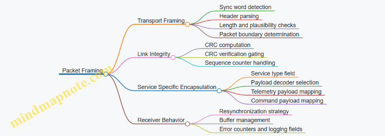
Receiver Flow with Integrated Checks
A systematic receiver flow prevents subtle bugs. The receiver should:
- Search for sync patterns in the incoming bit or byte stream.
- Parse the header and extract packet type, service type, and length.
- Apply plausibility rules: length within bounds, header fields within allowed ranges.
- Compute CRC over the exact header and payload bytes implied by length.
- If CRC passes, dispatch to the service decoder.
- If CRC fails, record the failure and continue searching from the next plausible boundary.
This approach avoids a common failure mode: accepting a packet because the sync detector was lucky, then crashing when the length field points outside your buffer.
Example: Minimal Field Layout and Validation Rules
Consider a simplified layout:
- 2 bytes: sync
- 1 byte: packet type (telemetry or command)
- 1 byte: service type
- 2 bytes: payload length
- N bytes: payload
- 2 bytes: CRC
Validation rules:
- Payload length must be between 0 and a configured maximum.
- Packet type must match the service type expectations.
- The total frame size must fit in the receive buffer.
- CRC must match before dispatch.
If you implement these checks in order, your framing layer becomes predictable, and your service decoders can assume they only see valid payloads.
Practical Notes for Ground Station Integration
In a ground station pipeline, framing sits between the demodulated bitstream and the higher-level telemetry/command handlers. That means it should produce structured outputs such as “packet accepted with metadata” or “packet rejected with reason.” Sequence counters and time tags should be carried alongside payloads so downstream logic can correlate measurements with tracking and scheduling data.
A small but useful habit is to keep framing decisions deterministic. Given the same input bytes, the framing layer should always produce the same accept/reject outcome and the same parsed header fields. That makes debugging far less mysterious, even when the RF chain is doing its best to be unpredictable.
10.2 Time Stamping Time Tags and Correlation with Tracking Data
Time stamping is the glue between what the receiver measures and what the antenna did. In a ground station, you typically have three clocks to reconcile: the RF/SDR sample time, the tracking system time, and the station computer time that labels packets for storage and analysis. If you treat time as an afterthought, you’ll still get data—just not the right data at the right moment.
Foundational Concepts for Time Alignment
Start with the idea that every measurement needs a time reference and a mapping from “hardware time” to “system time.” For SDR IQ samples, the timestamp usually marks either the first sample in a buffer or the center of a processing window. For tracking, timestamps often represent the moment the pointing command was issued or when the sensor reported position. Those are not the same event, so you must define which event each timestamp represents.
A practical rule: choose one “analysis timeline” (often the station computer time) and convert everything into it using recorded offsets and latencies. Latency is not a nuisance detail; it’s the reason correlation fails.
Time Tagging Models for SDR and Tracking
Use a consistent model for each data stream:
- SDR IQ time tags: store the sample index and the sample rate, then compute the absolute time for any sample as
t = t0 + n / Fs. Keept0andFswith the data. - Demodulation and decoding time tags: if you process in blocks, tag the block with the time of the block center or the first symbol boundary you can justify. Record the chosen convention.
- Tracking time tags: tag either the sensor measurement time or the command issuance time. If you have both, keep both; correlation improves when you can choose the correct one.
When you correlate, you’re matching events, not just timestamps. A good correlation uses the event definition that best matches the physical path: RF propagation delay plus internal processing delay plus any buffering delay.
Correlation Workflow from Raw Streams to Aligned Events
A systematic workflow prevents “mystery offsets”:
- Collect synchronization metadata: clock source identity, time offset estimates, and buffer sizes for SDR and tracking.
- Normalize timestamps: convert SDR and tracking times into the analysis timeline using the recorded conversions.
- Apply known fixed delays: for example, a known pipeline delay between IQ acquisition and demodulated symbol output.
- Estimate residual offset: compute the offset that maximizes a correlation metric, such as peak alignment between predicted and observed carrier phase rate or between beacon power bursts and pointing changes.
- Validate with sanity checks: confirm that the aligned events fall within expected physical bounds, like plausible Doppler rates and reasonable pointing error magnitudes.
A small example helps. Suppose your tracking system updates pointing every 20 ms, but your demodulator outputs frames every 10 ms. If you correlate frame timestamps directly to the latest tracking update, you’ll see a sawtooth pattern in pointing error. The fix is to interpolate tracking position to each frame time, using the two nearest tracking samples.
Mind Map: Time Tagging and Correlation
Concrete Example with Interpolation and Residual Offset
Assume tracking reports azimuth and elevation at times T0, T0+20ms, T0+40ms.... Your demodulator produces a frame at t = T0 + 13ms and t = T0 + 23ms. Nearest-neighbor mapping would assign the first frame to T0 and the second to T0+20ms, creating a discontinuity at 20 ms.
Instead, linearly interpolate pointing for each frame time using the two surrounding tracking samples. Then compute predicted line-of-sight geometry and compare it to observed metrics like received power or phase rate. If you still see a consistent offset—say, all predicted peaks occur 6 ms early—apply a residual time correction and re-check that the offset is stable across multiple passes or multiple beacons.
Data Quality Checks That Prevent Silent Errors
Before trusting correlation results, verify:
- Monotonicity: timestamps should increase within each stream.
- Buffer consistency: SDR metadata should match actual sample counts.
- Event definition consistency: the same convention must be used across the entire dataset.
- Residual offset behavior: if the estimated offset jumps wildly between segments, you likely have a missing metadata record or a stream restart.
A dataset labeled with correct times but inconsistent conventions is worse than a dataset with obvious gaps, because it produces confident-looking but wrong correlations. Treat time tags as first-class data, not labels you can casually regenerate.
10.3 Logging Monitoring and Alarm Threshold Design
A ground station produces more than packets and plots; it produces evidence. Logging and monitoring turn that evidence into quick answers: what happened, where it happened, and whether it matters right now. Threshold design is the bridge between raw measurements and operator action.
Foundational Logging Principles
Start by deciding what you must reconstruct after the fact. For each processing stage—RF capture, synchronization, demodulation, decoding, and telemetry framing—log three categories of information:
- State: configuration and mode changes (sample rate, LO plan, tracking state, coding mode).
- Measurements: numeric indicators (SNR estimate, carrier frequency offset, AGC gain, lock status).
- Events: discrete occurrences (sync acquired, frame lost, FEC decode failure rate crossed a limit).
A practical rule: every log line should answer one question without requiring another log line. For example, a “frame lost” event should include the frame index or timestamp window, the last known sync status, and the current frequency offset estimate.
Monitoring Signals That Matter
Monitoring should focus on indicators that correlate with link health and operational risk. Typical signals include:
- RF chain health: AGC gain level, front-end overload flags, IQ clipping indicators.
- Carrier and timing: frequency offset estimate, phase lock status, symbol timing error magnitude.
- Demodulation quality: soft-decision metrics summary, constellation sanity checks, demodulator confidence.
- FEC and framing: decode success rate over a sliding window, parity check statistics, frame sync acquisition rate.
- System performance: processing latency, buffer underruns, dropped IQ blocks.
Use sliding windows for anything that can fluctuate quickly. A single bad frame is usually noise; a sustained pattern is a problem.
Alarm Threshold Design Method
Design thresholds in layers: warning first, then critical. Each alarm should have a clear operator meaning.
- Define the window: e.g., 10 seconds for RF overload, 1 minute for decode success degradation.
- Choose the baseline: use a “known good” pass or a calibration period to establish typical ranges.
- Separate transient from persistent: require N consecutive windows before escalating.
- Account for operating mode: thresholds differ between acquisition and tracking, or between coding rates.
- Tie alarms to actions: each alarm should map to a short checklist (check LO stability, verify antenna pointing, reduce gain, restart sync).
A useful mental model is “sensitivity vs. usefulness.” If alarms trigger too often, operators stop trusting them. If they trigger too rarely, you learn about problems after the damage.
Example Threshold Set with Reasoning
Assume a coherent receiver with SDR baseband and FEC decoding.
-
Warning: IQ clipping
- Condition: clipping flag active for more than 1% of IQ blocks in a 10-second window.
- Reasoning: clipping often precedes decode degradation; catching it early helps adjust gain.
- Action: reduce RF gain or adjust AGC target; verify front-end headroom.
-
Critical: Loss of carrier lock
- Condition: carrier lock status false for 3 consecutive 10-second windows.
- Reasoning: short lock blips can happen during Doppler dynamics; three windows indicates a real failure.
- Action: verify LO control, check frequency plan, confirm antenna pointing stability.
-
Warning: Decode success rate drop
- Condition: FEC decode success below baseline minus 10 percentage points over 1 minute.
- Reasoning: success rate is a downstream indicator; using a relative drop avoids hardcoding for different links.
- Action: check SNR trend, confirm tracking quality, inspect interference flags.
-
Critical: Frame sync unavailable
- Condition: no valid frame sync detected for 2 consecutive 30-second windows.
- Reasoning: framing failure blocks telemetry; it is operationally urgent.
- Action: restart sync acquisition, verify preamble detection parameters, confirm time alignment.
Mind Map: Logging Monitoring and Alarm Threshold Design
Operational Checklist for Threshold Validation
Before deploying thresholds, validate them with recorded IQ and representative passes. Confirm that:
- Warnings trigger during controlled gain changes and recover after adjustment.
- Critical alarms trigger only when the system truly cannot maintain lock or framing.
- Alarms include enough context to act without opening a dozen dashboards.
A good threshold is one that makes the next step obvious. If the alarm fires but the operator still needs to guess what to check first, the threshold logic is incomplete.
10.4 Data Quality Metrics SNR BER PER and Link State Indicators
Why Metrics Need a Shared Meaning
Data quality metrics only help if everyone interprets them the same way. In a ground station, SNR is a physical-layer quantity, BER and PER are decoding outcomes, and link state indicators summarize whether the system is currently usable. The trick is to compute each metric from consistent time windows and to attach it to the same packet or frame boundaries used by the demodulator and decoder.
Mind Map: Metrics and Their Relationships
SNR: From Estimated Power to Actionable Numbers
SNR in practice is an estimate derived from IQ samples. A common approach is to compute signal power in a band around the expected carrier and noise power in adjacent bins that exclude the signal. For example, if your demodulator uses a 1 kHz symbol-rate channel and you process 10 ms frames, you can estimate SNR per 10 ms frame by:
- Apply the same frequency correction used for demodulation.
- Measure power in the expected occupied bandwidth.
- Measure noise power in guard bins and subtract any known leakage.
- Convert to SNR in dB.
Example: If signal-bin average power is 1.0 mW and noise-bin average power is 0.1 mW, SNR is 10 dB. If the next frame drops to 6 dB while tracking remains locked, the likely cause is fading or interference rather than a loss of lock.
BER: Counting Bits Without Fooling Yourself
BER requires bit-level decisions. If you have a known training sequence or pilot bits, you can count bit mismatches directly. If you only have payload bits, you can still estimate BER using CRC outcomes, but that estimate is indirect because CRC detects blocks, not individual bits.
Example with known bits: Suppose a frame contains 10,000 known bits and you observe 20 bit errors after FEC bypass or before FEC. BER is 20 / 10,000 = 2e-3. If you only have 200 known bits, the same 2 errors would yield BER 1e-2, but with much higher uncertainty. Reporting should include the number of evaluated bits so operators can judge whether a change is meaningful.
PER: The Packet-Level Metric That Matches Operations
PER is usually the most operationally relevant metric because ground software cares about whether packets are usable. Define PER as the fraction of packets failing CRC after the full demodulation and decoding pipeline. Use consistent packet boundaries: if frame sync slips by even a small amount, you can get a burst of PER without any real RF degradation.
Example: Over a 1-second window with 100 packets, 92 pass CRC and 8 fail. PER is 8%. If SNR is stable but PER spikes, suspect timing alignment, deinterleaving boundary issues, or a mismatch between expected coding parameters and received configuration.
Link State Indicators: Turning Metrics into a Coherent Status
Link state indicators combine lock status, decoding success, and quality thresholds into a small set of states. A practical scheme uses three layers:
- Acquisition state: carrier lock and timing lock status.
- Tracking state: residual frequency error and timing error within bounds.
- Decoding state: FEC success rate and CRC pass rate.
Example state logic for a 10 ms reporting cadence:
- Good: carrier lock true, timing lock true, CRC pass rate above 95%, and SNR above a configured minimum.
- Degraded: locks true but CRC pass rate between 80% and 95% or SNR near threshold.
- Lost: either lock false or CRC pass rate below 80% for a sustained window.
The “sustained window” matters. A single bad packet is normal; a run of failures indicates a real problem. Use the same window length for SNR, BER, and PER reporting so the state indicator doesn’t contradict the underlying metrics.
Example Reporting Bundle for One Time Block
A clean telemetry record for one time block should include:
- Start and end timestamps for the IQ window.
- SNR estimate in dB and the method identifier.
- BER estimate with evaluated-bit count or an explicit “not available” marker.
- PER with packet count and CRC failure count.
- Link state plus the lock flags used to compute it.
Example: “10:15:42.000–10:15:42.010, SNR 7.2 dB, BER not available, PER 3/50, state Degraded, carrier lock true, timing lock true.” This single line tells you the system is still synchronized but decoding is struggling, which is exactly the kind of information that prevents guesswork.
10.5 Practical Software Integration With SDR Processing and Storage
A ground station pipeline usually has three jobs: move IQ samples reliably, process them deterministically, and store results in a way that later you can actually find them. The easiest way to keep this sane is to treat the SDR as a streaming source with strict timing metadata, then build processing stages that consume and produce well-defined data products.
Start with a minimal data contract. Each buffer of IQ samples should carry: capture start time (or sample index), center frequency, sample rate, gain settings, and a unique run identifier. If you later correlate tracking telemetry with demodulation results, you will be grateful that you recorded the time base at the moment of capture, not after the fact.
Mind Map: SDR Processing and Storage Integration
Systematic Pipeline Layout
Use a producer–consumer pattern with bounded queues. The capture stage should never block on disk I/O. Instead, it pushes IQ buffers into a ring buffer; processing threads pop from the ring buffer, compute results, and forward only what you need to storage.
A practical split is:
- Capture: reads IQ from the SDR driver and timestamps buffers.
- Process: applies calibration (IQ imbalance and DC offset), runs frequency/timing estimation, demodulates, and performs FEC.
- Store: writes raw IQ only when needed (for debugging or commissioning), while always storing derived products like spectra snapshots, frequency offset traces, and decoded frames.
This keeps storage volume under control while still preserving enough evidence to troubleshoot.
Example: Chunking Strategy That Doesn’t Paint You into a Corner
Suppose you capture at 10 MS/s complex with 16-bit I and 16-bit Q. That’s 40 MB/s raw. If you store raw IQ continuously, you will fill disks quickly. A common approach is to store raw IQ in short windows around events.
Example policy:
- Always store derived outputs for the full pass.
- Store raw IQ only for 5-second windows when SNR drops below a threshold or when lock is lost.
To implement this cleanly, your processing stage emits an “event” message with the sample index range to store. The storage stage then requests the corresponding IQ chunks from the ring buffer.
Example: Metadata That Makes Post-Processing Possible
When you write a decoded frame, include:
- frame sequence number
- estimated carrier frequency offset and uncertainty
- symbol timing estimate
- FEC decoder mode and metric thresholds
- the exact configuration hash (SDR settings, filter taps, demod parameters)
This lets you re-run processing on the same raw IQ later without guessing which settings were used.
Storage Integrity and Verification
Add integrity checks at two levels:
- File-level: store a checksum per chunk and record chunk boundaries in an index file.
- Run-level: record counts such as number of IQ buffers captured, number processed, number dropped, and number of frames decoded.
During commissioning, verify that the number of processed samples matches the number of stored derived products. If they diverge, you likely have a queue overflow or a timestamp mapping bug.
Minimal Implementation Sketch
Below is a compact structure showing how capture, processing, and storage can communicate without blocking capture on disk.
RunController
  - config
  - run_id
  - start_time

CaptureThread
  - read IQ buffers
  - attach metadata
  - push to ring buffer

ProcessThread
  - pop IQ buffers
  - apply calibration
  - estimate freq/timing
  - demodulate and decode
  - emit DerivedProducts
  - emit StoreEvent when needed

StorageThread
  - write DerivedProducts
  - on StoreEvent, pull IQ chunks from ring
  - write RawIQ chunks with checksums
  - update run index
Practical Operational Workflow
A reliable run starts with configuration capture: write the SDR settings, filter parameters, and processing thresholds into a run manifest before the first buffer arrives. Then, log a small “heartbeat” record every few seconds containing current estimates (frequency offset, lock status, and throughput). When the run ends, close files with a final index update so the dataset is self-describing.
If you follow these rules—bounded queues, explicit metadata, event-driven raw storage, and chunk integrity checks—you get a pipeline that behaves predictably under real RF conditions, not just in ideal lab demos.
11. End-to-End Test Plans and Commissioning Procedures
11.1 Commissioning Stages From RF Bench Tests to Over The Air Tests
Commissioning is easiest when you treat it like a ladder: each rung proves one specific behavior, and the next rung builds on that proof. The goal is not to “get a signal,” but to confirm that the RF chain, timing, and baseband processing agree with the link plan.
Mind Map: Commissioning Stages
Stage 0: Preparation
Start by freezing the “known good” configuration: SDR sample rate, center frequency strategy, gain mode, filter bandwidth, and any calibration files. Define acceptance metrics before you measure, such as minimum carrier-to-noise ratio for lock, maximum frequency error after correction, and packet error rate thresholds for a short test window. This prevents the classic problem where everything “looks fine” until you need a pass/fail decision.
Stage 1: RF Bench Characterization
Use a signal generator and attenuators to emulate realistic power levels. First verify frequency behavior: tune across the expected band and confirm that the measured IF or baseband tone follows the plan without unexpected jumps. Next verify amplitude behavior: step input power in known increments and record the resulting ADC power and estimated SNR. If SNR improves linearly with input power over a useful range, your gain staging and noise figure assumptions are likely aligned.
Then check IQ health. Inject a single tone and measure DC offsets and I/Q gain/phase imbalance using your SDR’s calibration tools or a simple offline estimator. If imbalance is large, demodulated constellations will show systematic rotation or mirrored points even when SNR is high. Finally, verify filtering: sweep the tone frequency across the receiver bandwidth and confirm that gain roll-off and group delay do not break your demod assumptions.
Example: If your receiver uses a 20 MHz baseband bandwidth but the signal generator tone is placed 9 MHz off center, you should expect reduced amplitude due to filter shape. Record that reduction so later over-the-air comparisons aren’t confused with a “missing link.”
Stage 2: Controlled RF Loopback
A loopback proves end-to-end behavior without the uncertainty of propagation. Connect a transmit path to a receive path through a controlled attenuator and isolator so the receiver doesn’t saturate. Run a short burst test that includes acquisition, demod, and FEC decode. Acceptance here is not just “a decode happened,” but that acquisition time stays within your operational window and that the decoder output matches expected error statistics.
Stress the receiver dynamic range by varying loopback attenuation. Watch how AGC behaves: it should converge quickly and avoid hunting. If AGC oscillates, you’ll see unstable carrier recovery or fluctuating constellation quality. Also verify timing alignment if your processing uses symbol timing recovery; a consistent timing estimate across repeated bursts indicates your resampling and clock assumptions are coherent.
Example: For a QPSK test, run the same burst at three input levels. You should see constellation rotation remain stable after calibration, while the spread increases at lower SNR. If rotation changes with power, you likely have gain-dependent IQ imbalance.
Stage 3: Antenna and Feed Integration
Move from cables and benches to the antenna system. Measure and document RF losses from the feed to the receiver, including connector repeatability. Confirm polarization alignment by injecting a known tone and rotating polarization (or using a polarization switch) while monitoring received amplitude and demod quality. If the system supports beam steering, verify that the tracking interface updates pointing commands with the expected timing and that the antenna controller does not lag behind the baseband processing.
Example: If a polarization mismatch reduces received power by 6 dB, your link budget must reflect that loss. Don’t “fix it later” with higher transmit power unless you can also confirm the receiver won’t saturate during acquisition.
Stage 4: Over the Air Commissioning
Over-the-air tests use the real propagation environment, so you focus on acquisition and robustness. Begin with a beacon or test transmitter at a predictable schedule. Confirm that your frequency plan and Doppler correction converge: the carrier should lock, and the residual frequency error should remain within the demod’s tolerance.
Next validate packet integrity. Run repeated short transmissions and record packet error rate, not just raw constellation plots. If you see intermittent failures, correlate them with tracking telemetry such as pointing error and predicted Doppler rate. This often reveals whether failures are caused by beam mispointing, timing drift, or RF front-end saturation.
Example: During a pass, if packet errors spike when pointing error exceeds a threshold, you can treat that threshold as an operational constraint. If errors spike when received power is highest, suspect front-end compression or ADC clipping.
Stage 5: Operational Handover
Once acceptance criteria are met, freeze configurations and archive calibration artifacts used during commissioning. Create a short operator checklist that maps symptoms to likely causes: “no lock” points to frequency plan or LO stability, “lock but no decode” points to demod/FEC parameters, and “decode drops at high power” points to gain staging or compression. Record the final settings so the next test run starts from the same ground truth.
11.2 Verification Using Loopback Beacons and Known Reference Signals
Verification is easiest when you can separate “the RF chain works” from “the baseband and decoding work.” Loopback beacons and known reference signals let you do exactly that by injecting a controlled signal at a known point, then measuring expected outcomes at multiple checkpoints.
Foundational Concepts for Repeatable Verification
Start with three anchors: injection point, expected signal transformation, and acceptance criteria. The injection point is where the reference enters the system, such as an RF coupler feeding the receive chain or a baseband test tone feeding the SDR. The expected transformation describes what should happen between injection and measurement, including frequency translation, gain, filtering, and timing alignment. Acceptance criteria are numeric and specific, like “carrier frequency error within 1 kHz” or “EVM better than a chosen threshold.”
A practical mindset is to treat each checkpoint as a question:
- Does the signal arrive at the RF output with the right level and spectrum?
- Does the SDR produce the right center frequency and IQ balance?
- Does the demodulator recover the carrier and decode frames?
Loopback Beacon Verification Workflow
Use a loopback beacon when you want to test end-to-end without relying on a satellite link. The beacon can be a local transmitter that mimics the received waveform, or a controlled path that routes a transmitted signal back into the receiver.
-
Define the loopback mode Choose whether the loopback is RF-only, baseband-only, or full chain. RF-only isolates the front end; baseband-only isolates SDR processing; full chain checks everything together.
-
Set a reference operating point Pick one frequency, one modulation configuration, and one nominal receive level. Keep these fixed during the verification run so changes in results map to changes in the system, not to changing conditions.
-
Measure at the RF checkpoint Confirm the expected center frequency, bandwidth, and power level at the receiver output or an intermediate test port. If the spectrum shows unexpected spurs or a shifted carrier, stop before touching baseband settings.
-
Measure at the SDR checkpoint Verify that the SDR reports the same center frequency you expect after any mixing or direct sampling. Then check IQ imbalance indicators using a known tone or pilot, because IQ errors can look like “mysterious decoding failures.”
-
Measure at the baseband and decoder checkpoint Run the demodulator and record carrier lock metrics, frequency offset estimates, and frame synchronization success rate.
-
Compare results to acceptance criteria If any checkpoint fails, use the checkpoint hierarchy to localize the fault. For example, if RF power is correct but carrier lock fails, the issue is likely in LO stability, frequency planning, or IQ calibration.
Known Reference Signals That Map Cleanly to Symptoms
Known reference signals should be chosen so their failure modes are obvious.
- Single-tone references reveal LO offset, frequency plan errors, and gross IQ imbalance. If the tone appears mirrored or the image is strong, you likely have mixing or IQ sign issues.
- Modulated pilot references reveal demodulator and timing recovery behavior. If carrier lock succeeds but symbol timing fails, the waveform timing assumptions or resampling configuration may be wrong.
- Recorded IQ replays isolate software changes from RF hardware changes. If the same IQ file decodes correctly on one machine but not another, the difference is in processing configuration, not the RF chain.
Mind Map: Verification Using Loopback Beacons and Known Reference Signals
Example: A Systematic Pass-Fail Run
Assume you are verifying a full chain using a loopback beacon that transmits a QPSK pilot.
- RF checkpoint: You measure the carrier at the expected frequency and within the expected bandwidth. Power is within ±2 dB of the planned level.
- SDR checkpoint: The SDR center frequency matches the expected value after mixing. IQ imbalance indicators show no severe mirror component.
- Baseband checkpoint: Carrier lock occurs quickly, and the estimated frequency offset stays within your bound. Frame synchronization succeeds for a defined number of consecutive frames.
If frame sync fails but RF and SDR checkpoints pass, focus on demodulator configuration: symbol rate, filter bandwidth, and any resampling ratio. If carrier lock fails, revisit frequency planning and LO stability before changing FEC settings.
Example: Using a Single-Tone Reference to Catch IQ Sign Errors
Inject a single tone at a known offset from the expected center frequency. After processing, the tone should appear at the correct bin location in the spectrum. If the strongest component appears mirrored around the center frequency, the IQ sign or mixing polarity is wrong. Fixing this early prevents wasted time chasing “decoder problems” that are actually front-end math problems.
Practical Acceptance Checklist for Commissioning
Use a short checklist so results are comparable across runs:
- Injection point documented and consistent
- Frequency plan recorded with expected offsets
- RF power level within tolerance
- SDR center frequency aligned
- IQ imbalance within tolerance for the chosen reference
- Carrier lock achieved
- Timing recovery stable
- Frame sync and decode success meet the defined threshold
A commissioning run dated 2026-03-11 can be treated as a baseline: repeat the same procedure and compare checkpoint metrics rather than relying on a single “it works” outcome.
11.3 Performance Acceptance Criteria for Sensitivity and Throughput
Acceptance criteria for sensitivity and throughput should be written so a test engineer can answer two questions: “Will we detect the signal we care about?” and “Will we deliver the payload at the required rate?” The trick is to define the criteria in terms of measurable quantities that connect cleanly from RF chain behavior to decoded data.
Sensitivity Criteria That Survive Reality
Start with a link budget target expressed as required Eb/N0 or C/N0 at the demodulator input. Convert that into a testable receiver metric using your actual processing chain.
Define the sensitivity threshold as the minimum received signal level that achieves a specified packet success rate under stated conditions. Use a packet-based metric because it matches operational behavior and avoids arguing about “BER at infinity.” A common structure is:
- Test condition set: modulation, coding rate, symbol rate, bandwidth, Doppler scenario, and receiver mode (coherent/noncoherent).
- Success metric: packet success rate (PSR) over a fixed number of packets.
- Confidence: number of packets large enough that a single lucky burst does not decide the outcome.
- Margin: additional dB beyond the calculated threshold to cover measurement uncertainty and calibration residuals.
Example: Suppose the system requires PSR ≥ 0.99 for 1000 packets at a specified coding scheme. If your measured PSR at -124 dBm is 0.98 and at -123 dBm is 0.995, then -123 dBm is the sensitivity acceptance point for that configuration. If you also require 1.5 dB implementation margin, you would accept the design only if the sensitivity point shifts to at least -121.5 dBm after accounting for calibration and uncertainty.
Throughput Criteria That Match the Data Path
Throughput acceptance should be tied to end-to-end payload delivery, not just demodulated symbols. Define throughput as the effective payload rate after framing, error correction, and any required retransmission policy.
A practical throughput criterion includes:
- Target payload rate: e.g., 50 kbps net payload.
- Operating SNR region: specify the minimum and typical received levels for which the rate must hold.
- Latency bound: maximum time from first symbol detection to packet delivery, if your ground software expects timely processing.
- Processing headroom: ensure SDR compute load stays below a chosen utilization limit so bursts do not cause buffer overruns.
Example: If the demodulator can output frames at 200 frames per second but the FEC decoder and packetizer can only sustain 120 frames per second without backlog, then the throughput acceptance should be based on the sustained end-to-end rate. During testing, run a continuous stream for long enough to reach steady state, then verify that the delivered payload rate stays above the target while PSR remains within the sensitivity-defined region.
Measurement Setup and Uncertainty Budget
Sensitivity and throughput tests are only as good as the uncertainty accounting. Build an uncertainty budget that includes:
- RF level accuracy: signal generator power accuracy and any attenuator tolerance.
- Cable and connector effects: repeatability of insertion loss and return loss.
- SDR calibration residuals: IQ imbalance, DC offset, and gain flatness errors.
- Noise figure of the measurement chain: especially when using external noise sources or preamps.
Then apply a conservative rule: acceptance thresholds should include the combined uncertainty so you do not “pass” due to measurement optimism.
Mind Map: Acceptance Criteria Structure
Pass Fail Logic That Engineers Can Execute
Write the acceptance logic as explicit rules. For example:
- Sensitivity pass: PSR ≥ 0.99 for 1000 packets at the required configuration, with the tested received level meeting the threshold after subtracting combined uncertainty and adding required margin.
- Throughput pass: sustained net payload rate ≥ target for a continuous run of N seconds at the minimum required received level, with PSR not dropping below the sensitivity-defined requirement.
Example: If combined uncertainty is 0.8 dB and required margin is 1.5 dB, and the calculated sensitivity threshold is -124 dBm, then the tested acceptance level should be at least -124 dBm + 1.5 dB + 0.8 dB = -121.7 dBm (rounded to your test resolution). This turns a vague “it seems good” into a checkable statement.
Practical Test Matrix Without the Explosion
To avoid an unmanageable test matrix, group configurations by the parameters that most affect sensitivity and throughput: modulation/coding, bandwidth, and receiver mode. Keep Doppler scenarios limited to representative cases that stress acquisition and tracking behavior, and reuse the same compute and buffering settings across tests so throughput comparisons remain meaningful.
Example: If you have three modulations and two coding rates, test each modulation at the lowest and highest coding rate that changes decoder complexity, then run throughput at the sensitivity acceptance point for each modulation. This covers the main risk areas without multiplying tests by every possible combination.
Finally, record the acceptance criteria in a single place with the exact test conditions and the pass/fail rules. When the criteria are precise, the tests become repeatable, and the receiver stops being a mystery box that only works on good days.
11.4 Troubleshooting Signal Loss Causes from Antenna to Decode
When a satellite signal “disappears,” the fastest path to truth is to treat the receiver like a chain of measurable transformations. Start at the antenna and move downstream, verifying each stage with a specific observable: power, frequency, timing, constellation, or decoded frames. If you can’t measure it, you can’t fix it—so the goal is to reduce the problem to one link in the chain.
Mind Map: Signal Loss Triage from Antenna to Decode
Step 1: Verify Geometry and RF Capture
Begin with the antenna because it sets the ceiling for everything else. Confirm pointing using the same ephemeris and coordinate frames used for normal operations, then check polarization alignment if your system supports it. A common “it was fine yesterday” failure is an RF switch left in the wrong state, which can look like a total loss even when the rest of the chain is healthy.
Next, verify the LNA bias and its control path. If the LNA is off, you may still see noise, but your carrier-to-noise ratio will collapse. Measure received power at the earliest practical point (before major gain stages) and note whether the carrier appears at all.
Step 2: Confirm RF Chain Health with Measurable Signals
Move to the RF front end and treat each block as a hypothesis with an observable.
- Gain staging: If you see a carrier but decoding fails, check whether the receiver is saturating. Saturation often produces a “strong but wrong” spectrum: the carrier looks present, yet demodulation collapses due to nonlinear distortion.
- Filter mismatch: If the signal is present but shifted or broadened, verify the selected bandwidth and center frequency. A too-narrow filter can clip sidebands needed for acquisition.
- LO correctness: Verify LO frequency with a frequency counter or a reliable measurement path. A small LO error can move the signal out of the expected IF bin, causing acquisition to fail even though the spectrum still shows something.
- Imbalance and DC offset: If IQ imbalance is severe, you may see a carrier but the constellation rotates or collapses. DC offset can mask weak carriers during acquisition.
Step 3: Validate SDR Configuration and Data Integrity
If the RF spectrum looks right but baseband processing can’t find the carrier, check SDR settings.
Confirm sampling rate and decimation match the expected bandwidth. Then verify IQ ordering and data format. A classic failure mode is swapping I and Q or using the wrong endianness, which can produce a stable-looking spectrum but break phase-sensitive demodulation.
Also check for dropped samples or buffer underruns. These can create intermittent acquisition failures that look like “random” loss. If you log timestamps, compare them against expected sample counts to spot gaps.
Step 4: Prove Acquisition Parameters Match the Signal
At this stage, you should be able to see a carrier peak in the SDR spectrum. If acquisition still fails, focus on frequency and timing search.
- Frequency offset search range: Ensure the search covers expected Doppler and oscillator drift. If the true offset is outside the search window, the receiver will never lock.
- Doppler tracking settings: If tracking is enabled, confirm the model inputs and update rate. A mismatch can keep the signal just outside the tracking loop.
- Timing recovery: If you can detect carrier but not frames, timing recovery parameters may be off. Adjust symbol timing search ranges and loop bandwidth so the loop can settle within the observation window.
Step 5: Confirm Demodulation and FEC Mode Selection
If you reach demodulation but decoding fails consistently, treat configuration mismatch as the top suspect.
Verify modulation type, symbol rate, coding rate, interleaving mode, and frame structure. A wrong coding rate can yield plausible-looking soft metrics while still producing zero valid frames. Frame sync issues can also mimic “no signal,” because the decoder may reject everything before FEC even runs.
Soft decision scaling matters too. If the demodulator outputs hard bits but the decoder expects soft metrics, or if metrics are clipped too aggressively, FEC performance drops sharply.
Example: Carrier Present, No Frames
You observe a clear carrier peak in the SDR spectrum, but the decoder reports no valid frames.
- Check saturation: Reduce RF gain by a known step and re-run. If the constellation improves and frames start appearing, the original gain was too high.
- Check IQ integrity: Swap I/Q in software (or verify hardware cabling) and re-run acquisition. If lock improves immediately, the IQ path was inverted or misconfigured.
- Check mode mismatch: Confirm modulation and coding parameters against the mission configuration. If you accidentally selected a different coding rate, the decoder will never pass CRC.
- Check frame sync: Verify preamble detection thresholds and correlation settings. If the carrier is strong but correlation never peaks, the timing or symbol rate is wrong.
Example: No Carrier Peak
If you see only noise in the SDR spectrum, work upstream.
- Verify antenna pointing and polarization.
- Confirm LNA bias voltage and RF switch state.
- Check LO frequency and ensure the expected downconversion places the carrier inside the SDR capture band.
- Verify SDR center frequency and decimation so the capture window actually includes the expected IF.
Practical Troubleshooting Checklist
Use this order to minimize wasted time:
- Antenna pointing and polarization alignment.
- LNA bias and RF switch/T-R module state.
- RF gain staging for saturation avoidance.
- LO frequency correctness and filter bandwidth selection.
- SDR sampling rate, IQ ordering, and data integrity.
- Acquisition search ranges for frequency and timing.
- Demodulation mode and FEC parameters.
- Frame sync thresholds and soft metric scaling.
If you follow the chain and record what you observe at each step, the “mystery” usually turns into a single misconfiguration or a single hardware state. The receiver is rarely haunted; it’s usually just doing exactly what it was told.
11.5 Practical Test Scripts for Repeatable Measurements
Repeatable measurements come from controlling three things: the stimulus, the receiver state, and the measurement method. A good test script is basically a recipe with strict ingredient weights—except the ingredients are RF settings, timing, and calibration steps.
Define Success Metrics Before Touching Hardware
Start by writing down what you will measure and how you will judge it. For example:
- Sensitivity: minimum input level that achieves a target BER or packet error rate.
- Frequency accuracy: residual carrier offset after correction.
- Demodulation stability: how often lock is lost during a fixed-duration run.
- RF chain behavior: gain compression or phase drift under controlled input power.
Then choose pass/fail thresholds that match the mission’s operational needs. If you cannot state thresholds, you cannot tell whether a change helped or just moved the numbers around.
Build a Repeatable Test Environment
Before any RF stimulus:
- Fix the SDR configuration: sample rate, center frequency, gain mode, and buffer sizes.
- Fix the LO plan: record LO source type, tuning method, and any frequency correction mode.
- Lock the time base: ensure consistent timestamping and avoid mixing runs with different clock states.
- Standardize the RF path: use the same cables, attenuators, and connectors; note their serial numbers.
A practical habit: create a “run header” text block you paste into your log for every run. It should include every setting that affects the signal path.
Use a Scripted Measurement Flow
A repeatable flow has the same stages every time.
Stage A: Baseline capture
- With the RF input terminated or attenuated to a known low level, capture IQ for a fixed duration.
- Confirm noise floor stability and verify that DC offset and IQ imbalance are within expected bounds.
Stage B: Calibration stimulus
- Inject a known reference tone or modulated test signal at a mid-range power.
- Measure gain and phase response in the receiver chain.
Stage C: Sweep and verify
- Sweep input power across your region of interest using fixed step sizes.
- For each step, capture IQ and compute the same metrics.
- Re-check the mid-range point every N steps to detect drift.
Stage D: Decode validation
- Run the same demodulation and decoding pipeline settings for every step.
- Record lock acquisition time, number of lost frames, and final error metrics.
Mind Map of a Repeatable Script
Mind Map: Repeatable Measurement Script
Example Script Template for a Power Sweep
Use this structure for a sensitivity sweep with periodic drift checks.
Example plan
- Duration per step: 10 seconds IQ capture.
- Power sweep: from -120 dBm to -90 dBm in 2 dB steps.
- Mid-point re-check: repeat the -105 dBm step after every 5 steps.
- Metrics: packet error rate, residual carrier offset, and lock loss count.
Example run header fields
- SDR model and firmware version
- sample rate and center frequency
- gain mode and gain value
- LO source and any correction mode
- RF path identifiers and attenuator settings
- processing pipeline version and parameters
Outlier Rules and Rerun Criteria
Repeatability fails quietly when you accept bad runs. Define rules such as:
- If baseline noise floor shifts by more than a chosen margin, rerun baseline and abort the sweep.
- If lock is lost more than a set number of times at a given power, mark the step as “unstable” and rerun it once.
- If the mid-point re-check deviates beyond a threshold, stop and investigate drift before continuing.
A simple rerun policy prevents “chasing” results by adjusting settings midstream.
Practical Logging That Makes Results Auditable
Store results with consistent naming and include the run header in the same folder as the data. For each step, log:
- input power setting and measured reference level if available
- computed metrics with units
- processing configuration hash or parameter list
- any anomalies such as saturation indicators or unexpected frequency offsets
If you can’t reconstruct what happened from the log alone, the measurement is not repeatable—it’s just a story you told once.
Minimal Pseudocode for Script Control
for each step in sweep_plan:
  set_rf_power(step.power_dbm)
  wait_settle_time()
  capture_iq(duration_s)
  run_processing_pipeline()
  compute_metrics()
  save_step_results(step_id)

  if step.is_midpoint_recheck:
    compare_midpoint_to_baseline()
    if deviation_exceeds_threshold:
      abort_and_flag_run()
This structure keeps the receiver state consistent and ensures every step is measured the same way, which is the whole point of repeatable scripts.
12. Safety Grounding Compliance and Operational Reliability Engineering
12.1 RF Safety Practices Power Levels and Exposure Control
RF safety is mostly about controlling what reaches people: the field strength, the time it’s present, and the frequency-dependent way the body absorbs energy. In a satellite ground station, this means treating every RF path—amplifiers, waveguides, coax, antennas, and even “temporary” test setups—as potentially hazardous until proven otherwise.
Foundational Concepts for Exposure Control
Start with three practical ideas.
- Exposure depends on frequency and field distribution. At higher frequencies, energy couples differently into tissue, so the same power can produce different exposure levels. That’s why safety limits are frequency-specific.
- Exposure depends on time. A brief burst at a high level may be less risky than a longer transmission at a moderate level, assuming the same duty cycle and operating mode.
- Exposure depends on geometry. Distance, shielding, and antenna orientation matter. A “safe” power level at one distance can be unsafe at another.
A useful mental model is: power sets the potential, but distance, shielding, and operating mode decide what people actually receive.
Power Level Management That Actually Works
Power control should be layered, not single-point.
- Administrative controls: Define operating modes with maximum allowed transmit power and duration. For example, create a “commissioning mode” that caps output during alignment and a “service mode” that allows full power only when the antenna is in the correct configuration.
- Engineering controls: Use interlocks and RF shielding so the system cannot radiate at full power when doors are open or access panels are removed.
- Operational controls: Require a transmit authorization step that includes a quick check of antenna status, routing, and interlock state.
A concrete example: during antenna alignment, you might run at a reduced power and keep a person behind a barrier. If the interlock fails or the barrier is bypassed, the system should prevent full-power transmission rather than relying on someone remembering to “be careful.”
Exposure Control Workflow for Ground Station Operations
Use a repeatable sequence every time you change configuration.
- Identify the transmit path. Confirm whether RF is going to the antenna, a dummy load, a coupler, or a spectrum analyzer port. A coupler output can still leak RF if poorly terminated.
- Confirm termination quality. A dummy load must be rated for the frequency and power level, and it must be correctly connected. Loose connectors and mismatched loads are common sources of unexpected radiation.
- Check interlocks and indicators. Verify that door switches, access panel sensors, and “transmit inhibit” states are functional.
- Set the allowed power for the current mode. Apply the maximum transmit level for that specific task and duty cycle.
- Establish a controlled area. Define where people are allowed during transmit. Use signage and physical barriers so the boundary is not “whatever feels safe today.”
- Log the operating parameters. Record frequency, power setting, duty cycle, and the reason for transmit. This helps when troubleshooting also reveals safety-relevant faults.
Measuring and Verifying Safety Boundaries
Safety boundaries are not guesses. They are derived from measurements or conservative calculations, then verified.
- Survey approach: Use an RF field meter or appropriate measurement method at the boundary distance, at the relevant frequencies, and with the system in the intended transmit mode.
- Worst-case thinking: Treat the highest power mode and the most radiating configuration as the basis for the boundary. If the antenna pattern changes with polarization or pointing, verify the boundary for the configuration that produces the strongest exposure in the accessible area.
- Connector and leakage checks: Inspect and test transitions such as waveguide flanges, coax connectors, and enclosure seams. A small leak can matter when you’re near a boundary.
A practical example: if you run a high-power test into a directional coupler for monitoring, the coupler’s isolation and the termination on the monitor port determine whether the “monitoring setup” becomes the radiation source.
Interlocks and Fail-Safe Design
Interlocks should be designed so that faults reduce risk.
- Fail-safe behavior: If an interlock signal is lost, the system should inhibit transmit rather than defaulting to transmit.
- Independent verification: Where possible, use separate signals for “door closed” and “transmit enabled,” so a wiring fault doesn’t accidentally allow full-power output.
- Clear operator feedback: Indicators should state whether transmit is inhibited and why, so the operator doesn’t have to infer the system state.
Mind Map: RF Safety Practices Power Levels and Exposure Control
Example: Commissioning a New Transmit Chain Safely
- Start with a commissioning mode that caps transmit power and limits duty cycle.
- Route RF to a properly rated dummy load while verifying that interlocks inhibit transmit when access panels are open.
- Perform a boundary survey at the highest commissioning frequency and power.
- Only after the survey confirms the controlled area, switch to antenna routing for alignment, keeping the reduced power cap until alignment is complete.
- Increase to full service power only when the system is in the defined service mode and the interlock state is confirmed.
This sequence keeps the “unknowns” in the early steps, when you can still reduce power and control exposure with minimal operational complexity.
12.2 Grounding Bonding Lightning Protection and Surge Considerations
Grounding, bonding, and surge control are the quiet parts of a ground station that decide whether your RF chain behaves like a lab instrument or like a mystery novel. The goal is simple: keep all equipment at the same reference potential during normal operation, and control how currents flow during faults, lightning transients, and switching events.
Foundational Concepts That Drive the Design
Start with the difference between grounding and bonding. Grounding provides a path to earth; bonding ties conductive parts together so they share a common potential. In practice, you bond everything that can carry fault or transient current—rack rails, equipment chassis, cable shields, waveguide flanges, and antenna structure—so the transient current has a predictable route.
Next, treat surge behavior as a current-and-impedance problem, not a voltage problem. A surge current creates voltage across any impedance in the path, including cable shields, braid resistance, and connector contact resistance. Lower impedance and shorter paths reduce the voltage stress on sensitive front ends.
Finally, remember that lightning is not just “a big voltage.” It is a fast current pulse with energy that couples into conductors by direct strike, induced fields, and conducted paths through power and signal cables. Your job is to prevent that energy from turning into differential voltage across RF inputs.
Bonding Strategy for a Ground Station Rack
Use a single-point or multi-point bonding approach only if you understand the current paths. For most ground stations, a low-impedance bonding network is preferred over relying on one “special” connection.
A practical method:
- Create a main bonding bar near the entry points for power, RF coax, and control cables.
- Bond the antenna structure to this bar using wide conductors or multiple parallel straps.
- Bond each equipment rack to the bar with short, thick straps.
- Bond cable shields at the enclosure entry using 360-degree termination where possible.
Example: If your LNA module is mounted on a small bracket inside a rack, do not assume the coax shield alone provides bonding. Add a short bonding strap from the module enclosure to the rack bonding point so the shield current does not force the module chassis to float.
Lightning Protection System Interfaces
Lightning protection is typically implemented as a system: air terminals, down conductors, bonding to the building structure, and surge protective devices (SPDs). The key integration point is where the lightning current leaves the structure and where it enters your equipment.
Keep these rules:
- Down conductors should be straight and low-inductance, with minimal bends.
- Bond the down conductor to the main bonding bar so the current does not seek alternative paths through coax shields.
- Route RF coax and control cables away from down conductors when feasible.
Example: If a down conductor runs near the coax feed, the changing magnetic field can induce current in the coax shield. Even with good SPDs, that induced current can create a transient voltage across the receiver input reference.
Surge Considerations for Power and Control Lines
Power and control lines are common surge entry points. Use layered protection: SPDs at the service entrance, then at distribution panels, then at equipment power supplies. For control lines, protect at the I/O interface enclosure so the transient energy is handled before it reaches the SDR.
A systematic approach:
- Identify surge entry points: AC mains, DC supplies, Ethernet, serial/USB control, and any external sensors.
- Apply SPDs appropriate to each interface type.
- Ensure bonding continuity so the SPD discharge current returns to the bonding network without forcing equipment chassis to rise in potential.
Example: A network switch connected to the SDR via Ethernet can couple surge energy through the shield. Bond the Ethernet shield termination to the same bonding bar used for the rack, and use an appropriate Ethernet surge protector at the enclosure entry.
Cable Shield Termination and RF Chain Protection
For RF coax, shield termination quality determines whether surge current stays on the shield or leaks into the signal conductor. Use:
- 360-degree shield termination at the enclosure entry.
- Proper connector torque and clean mating surfaces.
- Short shield runs from the entry point to the bonding reference.
Example: If you terminate a coax shield with a pigtail, the inductance of that pigtail can produce a large transient voltage. Replace the pigtail with a clamp or bulkhead termination that maintains full circumference contact.
Verification Through Measurement and Documentation
You cannot “inspect your way” out of surge risk. Verify bonding continuity and transient path integrity.
- Perform continuity checks between chassis, rack, bonding bar, and shield terminations.
- Measure resistance of bonding straps and confirm they are not relying on paint or anodized surfaces.
- Document routing: where cables cross bonding conductors, where SPDs are installed, and which points are bonded.
Example: During commissioning, a continuity test reveals that one rack rail is isolated by a powder-coated fastener. Cleaning the contact surfaces and adding a dedicated bonding strap prevents that rail from becoming the return path during a transient.
Mind Map: Grounding Bonding Lightning Protection and Surge Considerations
Case Example: Preventing a Receiver Reset During a Nearby Discharge
A ground station experienced intermittent SDR resets during electrical storms. The RF chain still showed signal, but the control computer rebooted.
Systematic fix:
- Continuity testing found a control enclosure bonded through a painted mounting surface.
- The Ethernet shield was terminated with a partial clamp, leaving a gap.
- An SPD was installed, but the return path to the bonding bar was routed through a rack rail with high resistance.
Resolution:
- Cleaned and re-bonded the enclosure to the main bonding bar with a short strap.
- Replaced the Ethernet shield termination with a 360-degree enclosure entry termination.
- Re-routed the SPD return path to the bonding bar using a low-impedance conductor.
After changes, the SDR remained stable because surge current had a controlled path instead of creating a transient differential voltage across the control interface.
12.3 Environmental Protection Weatherproofing and Cable Management
Satellite ground stations live outdoors, indoors, and in the awkward middle where “mostly sheltered” is still exposed to wind-driven rain, condensation, and temperature swings. Weatherproofing and cable management are the practical disciplines that keep RF paths stable and prevent intermittent failures that show up only when the weather decides to cooperate.
Foundational Principles for Weatherproofing
Start with three rules: keep water out, keep moisture from migrating inside, and manage condensation when it inevitably forms. Water exclusion is about seals and correct installation; moisture migration is about preventing capillary paths along cable jackets and connectors; condensation control is about allowing trapped air to equalize pressure and temperature.
A common failure pattern is “it passed the bench test.” On the bench, connectors are dry and temperature is stable. In the field, a cable run can act like a straw: small gaps at a connector interface or an unsealed jacket edge can pull moisture inward. Once inside, the damage is often slow—corrosion at braid terminations, oxidation at contacts, and gradual degradation of shielding effectiveness.
Cable Routing and Mechanical Strain Control
Cable management begins before sealing. Route cables with gentle bends that respect the cable’s minimum bend radius, and avoid tight loops near moving antenna structures. Provide strain relief so connector loads never transfer to the RF interface.
Use separation between RF and power/control runs where practical. If they must share a tray, keep RF cables on the side with better physical shielding and maintain consistent spacing. This reduces coupling that can masquerade as “mysterious RF noise.”
Label both ends of every cable and record the mapping between antenna ports, RF chain inputs, and SDR capture channels. When a connector is replaced after a storm, you want to restore the exact path without guessing.
Weatherproofing Interfaces and Seal Strategy
Treat every interface as a potential leak point: connector backshells, gland entries, enclosure doors, and any penetration through a wall or radome support. The goal is not just to cover the outside; it is to stop water from reaching the first vulnerable boundary.
A practical seal strategy is layered:
- Primary barrier: a properly mated connector with correct torque and gasket condition.
- Secondary barrier: a weatherproofing boot or heat-shrink system that covers the full transition from connector to cable jacket.
- Tertiary barrier: enclosure sealing and drip loops so any water that reaches the outside cannot run along the cable toward the connector.
Drip loops matter because gravity is reliable. If a cable enters an enclosure from above, form a loop so water runs off the lowest point rather than continuing into the entry.
Condensation and Pressure Equalization
Temperature changes can pull moist air into enclosures through tiny pressure differences. If an enclosure is sealed too tightly without any equalization, it can “breathe” through the weakest seal during thermal cycling.
Use desiccant where appropriate and ensure any venting method is compatible with the environment. For cable runs that enter equipment housings, confirm that the entry method prevents moisture migration while still allowing safe thermal behavior.
Inside the RF chain, condensation is especially harmful because it can alter dielectric properties and promote corrosion at solder joints and connector contacts.
Shielding Continuity and Grounding at the Right Places
Weatherproofing must not break shielding continuity. When you seal a connector, ensure the braid termination remains intact and the shield path remains low impedance. A common mistake is to rely on the outer jacket for shielding after rework; the jacket is not a substitute for a proper shield termination.
Grounding should be intentional: bond shields to the designated reference points and avoid creating multiple uncontrolled ground loops. If you must bridge grounds for mechanical reasons, do it with a defined method rather than by letting water-resistant tape “decide.”
Example: Weatherproofing an Outdoor RF Cable Entry
Imagine an L-band coax run from an outdoor feed to an indoor enclosure. The cable enters via a gland.
- Route the cable so it forms a drip loop before the gland.
- Inspect the connector: confirm the gasket is present and undamaged.
- Apply a weatherproofing boot or heat-shrink over the connector-to-jacket transition, ensuring full coverage with no exposed jacket edge.
- Tighten the gland to compress the cable jacket without crushing it.
- Verify shielding continuity with a continuity check from braid to the enclosure’s reference point.
After installation, perform a simple functional check: monitor received signal strength during a controlled temperature change or after a light condensation event. If the link behaves differently, the issue is often a seal boundary or a grounding discontinuity.
Mind Map: Weatherproofing and Cable Management
Example: Troubleshooting After a Rain Event
If a receiver suddenly shows intermittent dropouts after heavy rain, follow the physical logic. First, check whether the issue correlates with enclosure openings, connector areas, or cable entry points. Then inspect for signs of jacket damage, loose glands, or missing boots. Finally, verify shielding continuity and connector seating.
Intermittent failures often come from water reaching a boundary and changing contact resistance. The fix is usually mechanical and sealing-related, not a software adjustment—because the RF chain is doing exactly what physics allows it to do when moisture gets involved.
12.4 Reliability Engineering for Fans Power Supplies and Cooling Paths
Reliability for a ground station is often decided by the boring parts: fans, power supplies, and the air path that moves heat away from RF hardware. Treat cooling as a system with failure modes, not as a background service.
Foundational Concepts for Cooling Reliability
Start with three quantities: heat load, airflow, and electrical stress. Heat load comes from RF amplifiers, mixers, SDR compute, and power conversion losses. Airflow is limited by filters, duct geometry, and fan aging. Electrical stress includes supply ripple, undervoltage events, and thermal cycling that loosens connectors.
A useful mental model is to separate “thermal capacity” from “thermal transport.” Thermal capacity is how much temperature rise the components can tolerate before performance or lifetime degrades. Thermal transport is how effectively the cooling path removes that heat. If either is weak, the system becomes sensitive to small changes like a clogged filter or a slightly slower fan.
Power Supply Reliability for Cooling Hardware
Cooling fans and their controllers usually run on DC rails that feed from a power supply. Reliability improves when you design for both steady-state and transient behavior.
-
Voltage regulation under load steps: Fans draw more current at startup and when bearings warm up. Choose supplies with stable regulation during load transients so the fan controller does not brown out.
-
Ripple and noise control: Fan drivers can inject noise into nearby analog front ends. Route fan power separately, add local bulk capacitance near the fan controller, and ensure the supply’s ripple stays within the controller’s tolerance.
-
Protection behavior: Overcurrent protection should fail safe. If the supply latches off, the cooling path stops and temperatures rise quickly. Prefer foldback or current limiting that allows the system to keep running while logging the event.
-
Thermal derating: Power supplies are rated at specific ambient temperatures. If the supply sits in the same airflow as the RF racks, use measured ambient values from commissioning and apply derating so the supply does not operate near its thermal limits.
Cooling Path Reliability Engineering
Cooling paths fail through airflow restriction, poor distribution, and heat recirculation.
-
Airflow restriction: Filters clog, intake screens collect dust, and cable bundles block flow. Design for serviceability: place filters where they can be replaced without disturbing RF alignment.
-
Airflow distribution: A fan can move air, but it may not deliver it to the hottest components. Use baffles or ducting so the flow reaches heat sinks and power modules.
-
Heat recirculation: Exhaust can be pulled back into intakes, especially in compact enclosures. Maintain separation between intake and exhaust zones and verify with smoke or airflow visualization during commissioning.
-
Thermal sensor placement: Sensors should represent the component temperatures that matter. A sensor mounted near a fan housing can look fine while the RF module overheats.
Systematic Failure Mode Coverage
Map failures to detection and response. For each failure mode, decide what the system should do and how you will know it happened.
- Fan failure: detect via tachometer feedback or airflow differential; respond by raising alarm thresholds and reducing compute or RF duty if your system supports it.
- Fan speed drift: detect by comparing tach speed to commanded PWM; respond by logging and scheduling maintenance.
- Supply undervoltage: detect via rail voltage monitoring; respond by holding critical modes until voltage recovers.
- Filter clogging: detect via rising temperature at multiple points plus stable fan speed; respond by alerting for filter replacement.
A good rule: detection should be based on independent signals. Temperature alone can be misleading if heat load changes; fan speed alone can be misleading if airflow is blocked.
Mind Map: Reliability Engineering for Fans Power Supplies and Cooling Paths
Example: Commissioning a Fan and Supply Setup
During commissioning, run a baseline thermal map at a defined operating mode. Record fan commanded speed, tachometer readings, supply rail voltage, and temperatures at the RF module heatsink, power supply intake, and the hottest compute area. Then simulate a clogged filter by partially restricting the intake while keeping fan speed control active.
You should see temperatures rise first at the component that depends most on that airflow branch. If instead all temperatures rise together, your airflow distribution is likely poor or sensors are not representative. Finally, verify alarm logic by forcing a fan speed mismatch and confirming the system logs the event and triggers the correct response.
Example: Designing for a Fan Controller Brownout
If the fan controller resets when the supply dips during fan startup, you get a loop: fan starts late, temperatures rise, and the controller may keep resetting. Fix it by adding local bulk capacitance at the controller input and selecting a supply with better transient response. Confirm the fix by measuring rail voltage during fan startup and verifying that the controller never resets under the same load step.
Practical Reliability Checklist for Cooling Paths
- Use measured ambient temperatures for derating power supplies.
- Place sensors on critical components, not just near airflow equipment.
- Verify airflow distribution with physical checks, not assumptions.
- Ensure protection behavior supports safe operation during faults.
- Correlate tachometer, rail voltage, and multi-point temperatures for detection.
- Log events with enough context to distinguish heat load changes from cooling degradation.
12.5 Practical Maintenance Schedules and Configuration Management
A reliable ground station is less about heroic fixes and more about predictable upkeep. The goal of maintenance scheduling is to keep RF performance stable, prevent avoidable downtime, and ensure that when something changes, you can explain why.
Maintenance Schedule Foundations
Start with a simple inventory: RF hardware, SDR platforms, timing and reference sources, antenna control electronics, and the software stack that ties them together. For each item, record failure modes you have actually seen or can reasonably anticipate: connector wear, fan failure, reference clock drift, SD card corruption, and misconfigured gain tables.
Use three maintenance tiers:
- Daily checks focus on “is it behaving right now.” Examples include verifying reference lock status, confirming that the receive chain gain settings match the current operating mode, and checking that the antenna controller reports expected position and limit switch states.
- Monthly checks focus on “is it drifting.” Examples include reviewing calibration logs for IQ imbalance and DC offset trends, inspecting cable strain relief and connector torque marks, and running a short RF loopback test at a known frequency.
- Quarterly checks focus on “is it degrading.” Examples include replacing aging fans, verifying power supply ripple under load, and confirming that the SDR host storage still sustains the required throughput without dropped buffers.
A practical cadence example: if you operate 5 days per week, do daily checks at the start of the first pass, monthly checks on the first non-operational day, and quarterly checks during a scheduled maintenance window.
Configuration Management That Prevents “It Worked Yesterday”
Configuration management is the discipline of making system state reproducible. Treat configuration as a first-class artifact, not a side effect of who last touched the system.
Define a configuration baseline for each operating mode, such as “Uplink Receive Mode” and “Downlink Transmit Mode.” Each baseline should include:
- SDR settings: sample rate, center frequency, front-end gain, decimation/interpolation, and any digital filters.
- RF chain settings: attenuator states, switch matrix positions, filter selections, and any calibration coefficients used.
- Timing settings: reference source selection, synchronization method, and expected lock indicators.
- Software versions: SDR application version, signal processing pipeline version, and any configuration files that define demodulation and decoding parameters.
Then enforce change control:
- Propose the change with a short reason and expected impact.
- Record the exact before-and-after values.
- Validate using a fixed test procedure that produces measurable outputs.
- Promote the new configuration to the baseline only after passing validation.
A simple rule: if a change affects RF gain, frequency plan, timing, or decoding parameters, it must be recorded as a new configuration revision.
Mind Map: Maintenance and Configuration
Concrete Examples That Make It Work
Example: Monthly calibration check with a decision rule. Run the same known reference signal test each month. Record the measured IQ imbalance and DC offset. If the change exceeds a defined threshold (for instance, a 20% increase in a specific coefficient compared to the last stable baseline), schedule an RF chain inspection before the next high-priority pass.
Example: Configuration revision for a gain table update. Suppose you adjust an SDR gain table to improve sensitivity at a specific elevation range. Create a new revision that includes the exact gain mapping, the RF attenuator states it assumes, and the decoding parameters used. Validate by running the same recorded IQ dataset through the pipeline and confirming that BER or packet error rate improves without increasing false lock events.
Evidence, Traceability, and Human-Readable Records
Maintenance is only as good as its records. Keep a single “system health” log that captures:
- What was checked.
- The measured results.
- Pass/fail outcomes.
- Any corrective actions taken.
For configuration, store revision IDs alongside the operational logs so that a later investigation can reconstruct the exact state. A good record answers three questions quickly: what changed, when it changed, and what test proved it was acceptable.
Finally, schedule maintenance tasks using a calendar that matches your operational reality. If you have a typical maintenance window on 2026-03-15, plan quarterly checks around that date so the team can reuse the same procedure, the same test signals, and the same acceptance criteria each time.