Engineering Vector Databases at Scale
1. Foundations of Vector Search and Retrieval Workflows
1.1 Vector Representations and Similarity Metrics
A vector database starts with a simple promise: if two items are “close” in meaning, their vector representations should be close in a chosen geometric space. The engineering work is choosing (1) how to represent items as vectors and (2) which notion of closeness to use.
Vector Representations
What a Vector Means
A vector is a fixed-length list of numbers. In practice, those numbers come from an embedding model that maps an input (text, image, audio, or structured fields) into a point in ℝ^d. The dimension d is fixed per model, so the system must keep that contract stable across ingestion and querying.
A useful mental model is that each dimension captures some latent factor, but you rarely interpret dimensions directly. Instead, you rely on the model’s training objective and on evaluation metrics to confirm that “nearby” points correspond to relevant items.
Common Representation Choices
- Dense embeddings: Every dimension has a value. This is the default for modern embedding models.
- Normalized embeddings: The vector is scaled to unit length, which makes cosine similarity behave like dot product.
- Multi-vector representations: Some systems store multiple vectors per item (for example, one per passage). This improves recall but complicates aggregation.
Practical Example
Suppose you embed product descriptions into 768-dimensional vectors. A query like “waterproof hiking boots” is embedded into the same 768-dimensional space. The system then compares the query vector to stored vectors and returns the nearest items.
Similarity Metrics
Similarity metrics define how to compare two vectors. The metric choice affects both retrieval quality and how you should preprocess vectors.
Cosine Similarity
Cosine similarity measures the angle between vectors:
- If vectors are unit-normalized, cosine similarity equals the dot product.
- Cosine similarity is often robust when vector magnitudes vary due to model behavior.
Example: If two descriptions point in similar directions in embedding space, cosine similarity will be high even if one vector has a larger norm.
Inner Product Similarity
Inner product is the raw dot product:
- It rewards both direction and magnitude.
- If you normalize vectors, inner product becomes equivalent to cosine similarity.
Example: If your model produces larger norms for certain categories, inner product may bias results toward those categories unless you normalize.
Euclidean Distance
Euclidean distance measures straight-line distance in \( ℝ^d \):
- It is sensitive to magnitude differences.
- If vectors are normalized, Euclidean distance is closely related to cosine similarity.
Example: Two items might be semantically similar but one embedding has a larger norm; Euclidean distance will treat them as farther apart.
Metric and Preprocessing Alignment
The most common engineering mistake is using a metric that doesn’t match your preprocessing.
- If you plan to use cosine similarity, normalize vectors during ingestion and query.
- If you plan to use inner product, decide whether magnitude should matter; if not, normalize.
- If you use Euclidean distance, ensure your vectors are in the scale you expect.
A quick sanity check is to run an offline evaluation: compare retrieval quality under each metric with the same embedding model and preprocessing. The best metric is the one that matches your relevance judgments, not the one that sounds mathematically elegant.
Mind Map: Vector Representations and Similarity Metrics
Worked Micro-Example
Imagine three stored vectors A, B, and C and one query Q. Suppose:
- A and B have similar directions to Q.
- C points in a different direction but has a larger norm.
With cosine similarity, A and B score higher because direction dominates. With inner product, C may score higher because magnitude contributes. With Euclidean distance, whichever vector is closer in straight-line distance wins, which often correlates with cosine only when vectors are normalized.
The takeaway is straightforward: metric choice is not a detail; it defines what “similar” means in your system. Once you lock in the metric, preprocess vectors accordingly and verify behavior with a small offline test before scaling up.
1.2 Retrieval Pipelines from Query Embeddings to Ranked Results
A vector retrieval system turns a user query into an embedding, searches an index, and returns a ranked list with enough context to be useful. The pipeline is easiest to reason about when you treat it as a sequence of transformations, each with clear inputs, outputs, and failure modes.
Step 1: Query Embedding Generation
The query text (or image, or structured input) is converted into a fixed-length vector using the same embedding model family used for documents. The practical detail that matters most is consistency: the embedding dimension, normalization behavior, and tokenization rules must match the document ingestion path. A common sanity check is to embed a known query and confirm that its nearest neighbors resemble what you expect from a small offline baseline.
Step 2: Candidate Generation via Vector Search
Candidate generation is where you trade accuracy for speed. You ask the index for the top k approximate nearest neighbors under a chosen similarity metric (often cosine similarity or inner product). The index returns IDs plus scores that are only meaningful relative to the candidate set.
A useful mental model: exact search gives you the true global top k, while approximate search gives you a “good enough” top k with bounded error. Engineers typically validate this by comparing recall at k against an exact baseline on a labeled set.
Step 3: Metadata Filtering and Hybrid Constraints
Real systems rarely retrieve purely by vector similarity. Filters such as tenant ID, language, document type, or time range reduce the search space. There are two main approaches:
- Filter-first: restrict the candidate pool using an inverted index or metadata store, then vector-search within the remaining IDs.
- Vector-first: retrieve candidates by vector similarity, then apply filters and possibly fetch more candidates if too many are filtered out.
Filter-first is often more predictable for strict constraints; vector-first can be faster when filters are loose. Either way, the pipeline must define what happens when fewer than k items survive filtering.
Step 4: Score Normalization and Rank Assembly
Scores from different shards, index variants, or distance conventions may not be directly comparable. If one component returns distances where “smaller is better” and another returns similarities where “larger is better,” you must unify the direction and scale.
A common approach is to convert to a consistent ordering key, then assemble results into a single ranked list. If you use cosine similarity, ensure embeddings are normalized the same way at both ingestion and query time; otherwise, the ranking can shift in surprising ways.
Step 5: Optional Reranking for Better Ordering
Candidate generation is optimized for speed, not perfect ordering. Reranking uses a second scoring function over the top n candidates (with n larger than k). This reranker can be a cross-encoder style scorer, a lightweight feature model, or a rules-based adjustment.
The key engineering detail is budget: reranking cost grows with n. A typical pattern is retrieve k or 2k candidates, rerank the top n (often close to k), then return the final top k.
Step 6: Fetching Payloads and Producing the Response
The index usually stores only vector-related metadata (IDs, maybe some lightweight fields). The pipeline then fetches the full payload—text snippets, titles, URLs, or structured fields—using the returned IDs. This step is where latency can quietly creep in, so batching and caching matter.
Finally, the response should include enough provenance to be debuggable: the final score, the candidate score, and which filters were applied. That makes it easier to explain why a result made the cut.
Mind Map: End to End Retrieval Pipeline
Example: A Concrete Pipeline with Numbers
Suppose you want the top k = 10 passages for a query.
- Embed the query into a 768-d vector.
- Ask the index for k’ = 50 candidates using cosine similarity.
- Apply a tenant filter that removes about 30% of candidates.
- If fewer than 10 remain, fetch an additional 20 candidates and repeat filtering.
- Normalize scores so higher means better.
- Rerank the top n = 20 candidates using a second scorer.
- Return the best 10 with payloads fetched in one batch by ID.
This example highlights why the pipeline needs explicit “what if” rules: filtering can reduce results, and reranking can change ordering even when candidate scores look close.
Example: Score Direction Mismatch Bug
Imagine one component returns distances where smaller is better, but the merge logic assumes larger is better. The system will still return k items, but they will be the worst matches. A quick prevention is to enforce a single internal convention: convert everything to a unified ordering key immediately after each scoring stage, then only merge using that key.
Step 7: Practical Validation Checklist
To keep the pipeline correct as it evolves, validate these invariants:
- Query embedding settings match document ingestion settings.
- Candidate generation returns enough items to survive expected filtering.
- Score direction is consistent across shards and rerankers.
- Payload fetching uses the same IDs returned by the ranking stage.
- Latency is measured per stage, not just end-to-end.
When these are in place, the pipeline becomes predictable: you can change one component and know exactly what should and should not move.
1.3 Indexing Versus Brute Force Search Tradeoffs
Brute force search compares a query vector against every stored vector, then sorts or partially selects the best matches. Indexing tries to avoid most comparisons by using structure: partitions, graphs, trees, or compressed representations. The tradeoff is simple to state and subtle to implement: brute force is predictable but expensive; indexing is fast but needs careful engineering to keep results accurate and stable.
Mind Map: Indexing Versus Brute Force Search
What Brute Force Gets Right
Brute force is the reference point because it is exact: if you compute the true distance for every vector, the top-k results are correct for that metric. That makes it ideal for debugging embeddings, verifying normalization, and building ground truth for evaluation.
It also has a clean performance model. If you store N vectors of dimension D, a single query performs O(N·D) arithmetic operations. On modern CPUs, the constant factors matter, but the linear dependence on N dominates as datasets grow.
Example: Suppose you have 10 million vectors, each with 768 dimensions. Even if each dimension comparison is cheap, you still do about 7.68 billion multiply-adds per query. If you need 100 queries per second, the arithmetic budget becomes the bottleneck long before you reach any clever ranking logic.
Why Indexing Exists
Indexing reduces the number of vectors you compare to the query. Most index types follow a pattern: use the query to find a small set of candidate vectors, then compute exact distances only for that candidate set (or compute approximate distances using compressed codes).
This changes the cost from O(N·D) to roughly O(C·D) where C is the number of candidates examined. The win is real when C is much smaller than N.
But indexing introduces two new sources of error and complexity:
- Candidate miss: the true nearest neighbor might not be in the candidate set.
- Distance approximation: the computed distance might be biased due to quantization or early stopping.
The Core Tradeoff Matrix
| Dimension | Brute Force | Indexing |
|---|---|---|
| Result correctness | Exact | Often approximate |
| Latency scaling | Linear in N | Depends on index and parameters |
| Memory | Store vectors only | Store extra structures and/or codes |
| Build time | None | Requires index construction |
| Updates | Simple but costly at query time | Often needs maintenance or rebuild strategy |
| Debugging | Straightforward | Needs evaluation and monitoring |
A Practical Example with Candidate Sets
Imagine two systems over the same dataset and metric.
- Brute force examines all N vectors and returns the exact top-k.
- Indexed search examines C candidates and returns the best among them.
If C is 50,000 for N = 10,000,000, you cut comparisons by 200×. The price is that recall depends on whether the index consistently routes the query to regions containing the true neighbors.
A useful engineering habit is to measure recall at multiple k values. A system might retrieve the correct top-1 rarely, but still retrieve the correct top-10 often enough for downstream reranking.
When Brute Force Still Makes Sense
Brute force is not “wrong”; it’s just expensive. It can be the best choice when:
- The dataset is small enough that linear scans fit your latency budget.
- You need an exact baseline to validate embeddings and normalization.
- You run offline evaluation where throughput matters less than correctness.
A common workflow is to start with brute force for correctness and metrics, then introduce indexing once you can quantify the gap between exact and approximate results.
Operational Implications You Can’t Ignore
Indexing is not just a faster query function. It adds lifecycle work: index build, parameter tuning, and maintenance under data changes. Even if the index is read-only, you still need to validate that the index version matches the embedding model version.
Brute force avoids these pitfalls because it depends only on the stored vectors and the distance function. That simplicity is why it remains a reliable tool for regression checks.
Mindful Decision Rule
Pick brute force when you need certainty and the dataset size allows it. Pick indexing when you need to meet latency and throughput targets and you can afford to engineer and measure recall. In practice, the best systems use both: brute force for ground truth and indexing for production retrieval.
1.4 Evaluation Metrics for Retrieval Quality and System Performance
A retrieval system has two jobs: return the right items and do it fast enough that the user experience stays steady. Evaluation metrics should therefore be split into quality metrics (did we find what matters) and performance metrics (how much it cost to get those results). The trick is to measure both with the same experimental discipline: fixed dataset splits, consistent query sets, and repeatable runs.
Quality Metrics for Ranking
Quality metrics start with a simple idea: each query has a set of relevant items, and the system produces a ranked list. If the relevant items appear early, the user usually benefits more than if they appear late.
Precision at k answers: “Of the top k results, how many are relevant?” Example: if k=10 and 7 of the top 10 are relevant, Precision@10 = 0.7.
Recall at k answers: “Of all relevant items, how many did we retrieve within the top k?” Example: if there are 20 relevant items total and 8 appear in the top 10, Recall@10 = 0.4.
Mean Average Precision (MAP) averages precision values computed at each position where a relevant item occurs. It rewards systems that not only find relevant items, but also interleave them well.
nDCG at k (normalized discounted cumulative gain) handles graded relevance. If you label items as {0,1,2} relevance levels, nDCG gives higher weight to correctly ranking the most relevant items near the top. Example: two systems might both retrieve the same number of relevant items, but the one that places the highest-grade items earlier gets a better nDCG.
MRR (mean reciprocal rank) is useful when there is typically one “best” item. Example: if the best relevant item is at rank 1, reciprocal rank is 1; at rank 5, it is 0.2.
A practical rule: if your application is “find the best answer quickly,” use MRR and nDCG. If it’s “collect useful candidates,” use Recall@k and Precision@k.
Quality Metrics for Filtering and Hybrid Retrieval
Vector search often includes metadata filters and reranking. Quality must reflect those constraints.
Filtered Precision and Recall compute metrics after applying filters. Example: if a query is restricted to a tenant and the system returns 10 items, Precision@10 should be computed only within that tenant’s relevant set.
Candidate Generation Recall measures how well the first stage (vector index) covers items that the reranker would like. Example: if the reranker’s top 20 includes 12 items that were present in the candidate set, then Candidate Generation Recall@20 is 12/20.
Reranking Lift compares quality before and after reranking on the same candidate lists. Example: if nDCG@10 improves from 0.42 to 0.48, the lift is +0.06.
System Performance Metrics
Performance metrics should be measured end-to-end, not just inside the index.
Latency percentiles (p50, p95, p99) show tail behavior. Example: p95 latency of 80 ms means 95% of queries finish within 80 ms; p99 of 200 ms flags occasional slow paths.
Throughput is queries per second under a defined concurrency level. Example: 500 qps at concurrency 64 is not the same as 500 qps at concurrency 8.
CPU and memory utilization help explain why latency changes. Example: if p99 spikes correlate with memory pressure, you may be thrashing caches or triggering garbage collection.
Index build time and refresh cost matter for operational workflows. Example: if compaction takes 30 minutes and blocks queries, you need a metric that captures the impact window.
Stability metrics include error rates and timeouts. Example: if 0.5% of queries time out, quality metrics become less meaningful because the system is not consistently returning results.
Experimental Design for Reliable Comparisons
To compare index variants fairly, keep the following constant: query embeddings, candidate set size (where applicable), reranker model version, and filter logic. Use the same ground truth labels for all runs.
When multiple metrics disagree, interpret them with intent. Example: a system might increase Recall@100 but reduce Precision@10. That often means it retrieves more items but ranks them less sharply.
Mind Map: Metric Selection
Example Metric Sheet for One Query Set
Assume 1,000 queries with binary relevance labels.
- Quality: Precision@10 = 0.31, Recall@10 = 0.18, nDCG@10 = 0.44, MRR = 0.29.
- Hybrid: Candidate Generation Recall@50 = 0.62, Reranking Lift nDCG@10 = +0.07.
- Performance: p50 latency = 35 ms, p95 = 80 ms, p99 = 200 ms, throughput = 520 qps at concurrency 64.
If Precision@10 is low but Recall@10 is decent, the ranking stage needs improvement. If Recall@10 is high but latency tails are bad, the index might be correct but inefficient under load.
Diagram: Metric Flow from Query to Decision
    flowchart TD
  Q[Queries] --> E[Embed Queries]
  E --> F[Apply Filters]
  F --> C[Candidate Generation]
  C --> R[Optional Reranking]
  R --> L[Ranked Results]
  L --> Qm[Quality Metrics]
  L --> Pm[Performance Metrics]
  Qm --> D[Decision on Tradeoffs]
  Pm --> D
Putting It Together
A good evaluation run produces a small set of metrics that answer concrete questions: “Are relevant items near the top?” and “Can we serve them reliably within our latency budget?” Once those are clear, you can use additional metrics like reranking lift and tail latency to pinpoint where the system is winning or losing.
1.5 Data Modeling for Documents Images and Structured Metadata
Vector search works best when the stored vectors and the stored meaning agree. Data modeling is the part where you decide what “meaning” looks like for documents, images, and structured fields, and how that meaning survives ingestion, updates, and filtering.
Core Modeling Principles
Start with three layers that stay separate but work together:
- Identity: a stable primary key for each item, plus versioning fields so you can reason about updates.
- Content: the raw text, image bytes, or extracted features you may need for debugging and reprocessing.
- Retrieval View: the vectors and metadata fields used for indexing, filtering, and ranking.
A practical rule: store enough raw content to reproduce embeddings, but keep the retrieval view optimized for fast queries. If you can’t rebuild embeddings from stored inputs, you’ll eventually be stuck with “mystery vectors.”
Document Text Modeling
For text documents, model both the embedding unit and the retrieval unit.
- Embedding unit: what you embed, such as a paragraph, section, or sliding window chunk.
- Retrieval unit: what you return, such as a chunk with a pointer to the parent document.
Example: a policy document becomes 200 chunks. Each chunk stores:
doc_id: stable document identifierchunk_id: unique within the documentembedding: vector for that chunkparent: fields likepolicy_typeorjurisdictioncopied from the parent for filteringtext: the chunk text for snippet display
This avoids a common failure mode: returning a parent document when the vector actually represents a chunk, which makes snippets feel unrelated.
Image Modeling with Captions and Regions
Images need a modeling decision: do you embed the whole image, regions, or both?
A robust approach is two retrieval views:
- Global view: one vector per image using a caption or a pooled image embedding.
- Local view: vectors per region or per detected object, each tied to bounding boxes.
Example: a product photo yields a global caption (“red running shoe on a white background”) and three region captions (“shoe toe,” “shoe laces,” “brand logo”). You store:
image_idview_type:globalorregionbbox: for region entriesembeddingcaption: the text used to create the vector
When a query matches a region vector, you can highlight the bounding box. When it matches the global vector, you show the whole image.
Structured Metadata Modeling
Structured metadata should support two tasks: filtering and ranking signals.
- For filtering, prefer fields that are stable and low-cardinality when possible, such as
tenant_id,language,doc_type,category, oraccess_level. - For ranking signals, store numeric fields like
timestamp,quality_score, orpopularity, and use them in reranking rather than in the vector index itself.
Example: a support ticket collection might store:
tenant_idlanguagestatus:open,closedcreated_atpriority: integer
Filtering uses tenant_id, language, and status. Reranking can incorporate priority and recency.
Hybrid Modeling for Mixed Modalities
When text and images share a collection, keep a consistent schema for retrieval view fields:
item_id: stable identifiermodality:text,image_global,image_regionembeddingmetadata: a uniform map of filterable fieldspayload: the display data (snippet text, image reference, or bbox)
This uniformity prevents query code from turning into a pile of special cases.
Mind Map: Data Modeling Components
Example Schema and Query-Time Behavior
A clean schema for retrieval entries might look like this:
item_idversionmodalityembeddingfilter_fields(object)payload(object)chunk_idorregion_id(optional)parent_id(optional)
At query time, you:
- Embed the query.
- Apply filter fields to restrict candidate entries.
- Retrieve top candidates by vector similarity.
- Rerank using ranking fields and payload-aware logic.
Example behavior: if the user requests language=fr and modality=image_region, the system filters to region entries only, retrieves by vector similarity, and then reranks by recency using created_at.
Update and Consistency Modeling
Model updates explicitly. If you re-embed with a new embedding model, treat it as a new version and keep old versions until you finish migration. Deletions should be version-aware so you don’t resurrect stale entries during compaction or rebuild.
A practical workflow:
- Ingest new content with
version = current_embedding_version. - Build or update the index for that version.
- Mark old versions as inactive.
- Ensure queries only consider active versions.
This keeps retrieval consistent and makes debugging less of a scavenger hunt.
2. Data Preparation and Embedding Management for Production Systems
2.1 Embedding Generation Pipelines and Deterministic Reproducibility
Embedding generation looks simple until you try to reproduce results months later, across machines, batch sizes, and model versions. This section treats the pipeline as an engineering system: inputs become embeddings through a sequence of deterministic transformations, and every transformation has a traceable contract.
Core Pipeline Stages
A production embedding pipeline typically has five stages.
- Ingestion and canonicalization: Convert raw content into a stable representation. For text, this means consistent Unicode normalization, whitespace rules, and a fixed truncation policy. For images, it means a fixed resize/crop strategy and color space handling.
- Tokenization and preprocessing: Apply the model’s tokenizer rules exactly. If you do any extra preprocessing (lowercasing, stripping markup, removing boilerplate), define it as a pure function.
- Model inference: Run the embedding model with fixed settings. Determinism depends on more than the model weights; it also depends on inference configuration.
- Post-processing: Apply normalization, projection, or quantization. If you normalize vectors, do it consistently (for example, L2 normalization) and document the exact math.
- Persistence and indexing readiness: Store embeddings with metadata that allows you to verify they match the same pipeline run.
A practical rule: every stage should be either deterministic by construction or explicitly versioned so you can replay it.
Determinism Targets and What Breaks Them
Deterministic reproducibility means that the same input produces the same embedding bytes under the same pipeline definition. In practice, you can aim for determinism at three levels.
- Exact determinism: Bit-identical embeddings. This is hardest when hardware kernels or floating-point behavior vary.
- Numerical determinism: Embeddings match within a tight tolerance. Often sufficient for retrieval, but you must measure it.
- Semantic determinism: Retrieval results remain stable even if embeddings differ slightly. This requires evaluation, not just math.
Common sources of nondeterminism include:
- Mixed precision (FP16/BF16) and dynamic loss scaling.
- Non-deterministic GPU kernels.
- Threading differences that change reduction order.
- Batch-dependent preprocessing such as padding or truncation done inconsistently.
- Random operations like dropout left enabled.
The fix is not “turn everything off,” but to set inference to evaluation mode, lock preprocessing, and control numeric behavior.
Deterministic Configuration Checklist
Use a configuration object that is stored alongside embeddings. Include:
- Model identity: model name, exact weights hash, tokenizer version.
- Inference settings: device type, precision mode, batch size, and any determinism flags.
- Preprocessing rules: normalization steps, truncation length, image resize/crop parameters.
- Post-processing math: normalization type, epsilon values, rounding rules.
- Runtime constraints: thread counts and any environment variables that affect math.
A small but effective habit: log the configuration as a canonical JSON string and hash it. That hash becomes part of the embedding record.
Example: Text Embedding with Canonicalization and Stable Truncation
Suppose you embed product descriptions. You want the same description to yield the same embedding even if it arrives with different whitespace.
- Canonicalization: normalize Unicode, collapse repeated whitespace to a single space, trim ends.
- Truncation: truncate by tokens to a fixed maximum, not by characters.
- Post-processing: L2 normalize the final vector.
If you later see retrieval drift, you can compare the stored pipeline hash and the stored canonical text hash to pinpoint whether the change was in preprocessing or in model inference.
Example: Image Embedding with Fixed Resize and Crop
For images, nondeterminism often comes from preprocessing. Define:
- Resize to a fixed short side.
- Center crop to a fixed resolution.
- Convert to a fixed color space.
- Use a fixed interpolation method.
Then store the preprocessing parameters and the image preprocessing hash with the embedding.
Mind Map: Deterministic Embedding Pipeline
Verification Workflow That Catches Real Problems
Determinism is proven by replay, not by intention. A simple workflow:
- Pick a small set of representative inputs.
- Run the pipeline and store embeddings plus pipeline config hash.
- Re-run the pipeline on the same inputs using the stored config.
- Compare embeddings:
- If you require exact determinism, compare bytes.
- Otherwise compare with a tolerance and record the maximum deviation.
If the comparison fails, inspect which stage changed by comparing input canonical hashes, tokenizer outputs, and post-processing outputs. This narrows the search quickly, because each stage has its own stable intermediate representation.
Practical Data Contracts for Reproducibility
Treat embeddings as outputs of a contract:
- Input contract: canonical input hash and raw input identifier.
- Pipeline contract: pipeline config hash and stage versions.
- Output contract: embedding vector bytes and post-processing parameters.
When you store these together, you can reproduce embeddings for debugging, backfills, and index rebuilds without guessing what changed. The pipeline becomes boring in the best way: predictable, inspectable, and consistent.
2.2 Normalization Strategies for Cosine and Inner Product Similarity
Normalization is the quiet step that decides whether your similarity scores behave like what you think they mean. Two common goals show up in vector search: (1) compare directions regardless of vector length (cosine similarity), and (2) compare raw dot products (inner product). In practice, many systems use inner product indexes, so normalization becomes the bridge between “directional similarity” and “dot-product machinery.”
Core Idea: Length Matters Unless You Remove It
For vectors \(x\) and \(y\), the dot product is \(x\cdot y = |x||y|\cos(\theta)\). If you want similarity to depend only on \(\theta\), you must remove the \(|x||y|\) factor. That is exactly what \(\ell_2\) normalization does: \(\hat{x} = x/|x|\). Then \(\hat{x}\cdot \hat{y} = \cos(\theta)\).
If you do not normalize, inner product similarity mixes direction and magnitude. That can be useful when magnitude encodes something meaningful (for example, confidence or frequency), but it can also create accidental bias where longer embeddings dominate rankings.
Mind Map: Normalization Choices and Their Effects
L2 Normalization for Cosine Similarity
The standard approach is to normalize every stored vector and every query vector with the same rule. A typical implementation computes \(|x| = \sqrt{\sum_i x_i^2}\) and then divides by it.
A practical detail: embeddings can occasionally be all zeros or extremely small due to upstream preprocessing. Dividing by a near-zero norm creates huge values and wrecks ranking. A common safeguard is to use an epsilon floor: if \(|x| < \epsilon\), either keep the vector as zeros or skip normalization and treat similarity as undefined. For retrieval, keeping zeros is usually safer because it prevents NaNs and keeps behavior consistent.
Inner Product Indexes with Cosine Semantics
Many vector indexes are optimized for inner product. If you normalize vectors to unit length, inner product becomes cosine similarity. This is not just a mathematical equivalence; it also makes score ranges predictable. With unit vectors, cosine similarity lies in \([-1, 1]\), so thresholds and debugging become less confusing.
Example: Suppose you have two candidates \(a\) and \(b\) and a query \(q\).
- Without normalization, \(q\cdot a\) might be larger simply because \(|a|\) is bigger.
- With normalization, \(\hat{q}\cdot \hat{a}\) depends only on the angle between them.
This difference shows up immediately when you log norms: if norms vary widely, unnormalized inner product often produces rankings that track norm more than direction.
When Not to Normalize
If your embedding model produces vectors where magnitude carries information, normalization removes that signal. For instance, some pipelines scale embeddings based on document length or confidence. If that scaling is intentional, using raw inner product can be correct.
A quick sanity check is to compute retrieval quality twice on a labeled set: once with raw inner product, once with unit normalization. If the best model relies on magnitude, normalization will usually reduce recall at fixed latency.
Consistency Rules That Prevent “Why Is It Different in Production”
Normalization must be applied consistently at both indexing and query time. If you index normalized vectors but query unnormalized vectors, the dot product becomes \(|q|\cos(\theta)\), reintroducing magnitude into the score. That can cause systematic ranking shifts even when the embedding model is unchanged.
Also ensure evaluation uses the same normalization pipeline. Ground truth labels are about the task, but the similarity function used to compute candidate sets must match the one used in the system.
Numerical Stability and Implementation Notes
Use float32 for storage if your system does, but compute norms in float32 or float64 depending on your tolerance for rounding. The key is to avoid NaNs and to keep the normalization rule deterministic.
Here is a compact normalization pattern:
import numpy as np

def l2_normalize(x, eps=1e-12):
    x = np.asarray(x, dtype=np.float32)
    norm = np.linalg.norm(x)
    if norm < eps:
        return np.zeros_like(x)
    return x / norm
Practical Example: Debugging with Norm Statistics
Imagine you see unstable top-k results across deployments. Start by checking norm distributions for stored vectors and queries. If stored norms cluster tightly but query norms vary, you likely have a normalization mismatch. If both vary, decide whether magnitude should matter for your task; then choose either unit normalization for cosine semantics or raw inner product for magnitude-aware scoring.
Normalization is not a cosmetic step. It defines the geometry your index is searching, and it defines what “similar” means in the first place.
2.3 Handling Updates Deletes and Re-Embedding Workflows
Vector systems rarely stay still. Documents change, embeddings drift as models evolve, and deletes must stop showing up in retrieval results. A good workflow treats updates and deletes as first-class events, not as afterthoughts.
Core Idea: Treat Embeddings as Derived Data
Embeddings are computed from source content plus configuration (model version, preprocessing, pooling, normalization). That means an embedding record is only valid for a specific “derivation recipe.” When the recipe changes, you either re-embed or explicitly route queries away from stale vectors.
A practical pattern is to store:
- A stable document identifier (doc_id)
- A vector identifier (vector_id) tied to a specific embedding recipe
- Metadata fields used for filtering
- A lifecycle state (active, deleted, superseded)
Update Semantics: Replace, Version, or Both
Updates can be handled in two common ways.
- Replace in place
- You overwrite the existing vector for doc_id.
- Simple, but you must ensure queries never see a half-updated state.
- Best when you can update atomically and you have low write concurrency.
- Version and supersede
- You insert a new vector_id for the same doc_id.
- The old vector is marked superseded.
- Queries filter to active vectors, and you clean up later.
- This is safer under concurrency and supports gradual rollouts.
A hybrid approach is common: version on write, then compact superseded vectors during index maintenance.
Delete Semantics: Soft Delete First, Hard Delete Later
Deletes should be visible immediately to retrieval. Hard deletion is often delayed because indexes and caches may still reference older vectors.
Use a two-step lifecycle:
- Soft delete: mark doc_id as deleted so retrieval excludes it.
- Hard delete: remove vectors and payloads after index compaction and cache invalidation.
This avoids “ghost results” where a user searches for something that was deleted seconds ago.
Re-Embedding Triggers: Model and Pipeline Changes
Re-embedding is required when the embedding recipe changes. Typical triggers include:
- Embedding model version changes
- Preprocessing changes (tokenization, truncation rules)
- Normalization changes (for cosine vs inner product)
- Dimensionality changes
To keep operations sane, tag each vector with embedding_recipe_id and ensure retrieval knows which recipe(s) are eligible.
Mind Map: Update Delete and Re-Embedding Workflow
Example: Versioned Updates with Atomic Visibility
Imagine doc_id=42 changes. You compute a new embedding and insert vector_id=9001 with embedding_recipe_id=R7. You then mark vector_id=8800 as superseded.
Retrieval should only consider vectors where:
- lifecycle state is active
- embedding_recipe_id is allowed for the current query routing
If you route queries by recipe, you can keep R6 vectors searchable until the new index is built, while still ensuring doc_id=42 returns the newest active vector.
Example: Delete Event Without Ghost Results
A user deletes doc_id=77. Immediately, you set lifecycle state for doc_id=77 to deleted. Even if the index still contains the old vector, retrieval applies a filter that excludes deleted doc_ids.
Later, during compaction, you remove the deleted vectors from the index and payload store. At that point, caches that might still contain stale candidates should be invalidated or naturally expire.
Example: Re-Embedding During a Recipe Migration
Suppose you move from recipe R6 to R7 on 2026-02-15. You can run a controlled migration:
- New writes use R7 immediately.
- Existing docs are re-embedded in batches.
- Retrieval allows both R6 and R7 during the transition, but only returns the active vector per doc_id.
This prevents a doc from appearing twice with different embeddings and keeps ranking consistent with the chosen recipe set.
Operational Checklist That Prevents Common Bugs
- Ensure every vector write is tied to a recipe id.
- Ensure lifecycle filtering is applied before returning results.
- Ensure superseded vectors are never treated as active.
- Ensure delete events update the same doc_id key used by retrieval.
- Ensure index refresh and compaction remove only what lifecycle says is safe.
When these rules are consistent, updates and deletes behave predictably even under concurrency. The system stops being “eventually correct” and becomes “correct by construction,” which is a nicer kind of boring.
2.4 Schema Design for Metadata Filters and Hybrid Retrieval
Vector similarity alone rarely satisfies real queries. People ask for “the same thing, but only from this tenant, time window, and document type.” Schema design is where those constraints become fast, predictable operations rather than expensive post-processing.
Core Concepts That Shape the Schema
A metadata filter schema has three jobs: (1) represent constraints clearly, (2) map constraints to efficient access paths, and (3) keep the filter semantics consistent across indexing and retrieval.
Start with a small set of metadata fields that are truly filterable. For each field, decide its type and cardinality. Low-cardinality fields like doc_type or language are ideal for bitset-style filtering. High-cardinality fields like user_id or session_id often require inverted indexes or routing strategies. Time fields benefit from range-friendly encodings and partitioning.
Hybrid retrieval means you combine vector candidates with metadata constraints and sometimes a keyword stage. The schema should support both: vector storage for embeddings and metadata indexes for filtering and keyword matching.
Mind Map: Metadata Fields and Retrieval Roles
Designing Metadata Fields for Efficient Filtering
Use a consistent naming convention and store metadata in a way that supports both exact and range predicates.
Tenant and authorization fields. Put tenant_id (and any required access scope) in every record. Even if your application enforces access, the retrieval layer should be able to filter by it so you can safely run shared infrastructure.
Document type and language. Store doc_type and language as categorical strings or small integers. If you expect frequent filtering on these fields, precompute per-value bitsets during indexing. Example: a query with doc_type in {invoice, receipt} becomes a fast union of two bitsets.
Time ranges. For timestamp, store both the raw value and a normalized bucket if you frequently query by “last N days.” Buckets reduce the number of range checks. Example: timestamp >= now-30d can map to a set of daily buckets, then refine within those buckets if needed.
Filter Semantics That Avoid Surprises
Define how each operator behaves. Common operators include equality, set membership, and ranges.
- Equality:
language = 'en' - Set membership:
doc_type in ['invoice','receipt'] - Range:
timestamp between [2026-02-01, 2026-02-28]
Use deterministic rules for missing fields. For instance, if a record lacks language, decide whether it should be excluded by language='en' or treated as unknown. Make that decision explicit in the schema contract.
Hybrid Retrieval Schema: Candidate Generation with Constraints
A practical flow is: compute the filter mask, generate vector candidates within that mask, then optionally rerank.
Example schema.
id(string)tenant_id(int)doc_type(int)language(int)timestamp(int64)embedding(float vector)text(optional for keyword stage)
Example query. “Find similar documents to this embedding, but only tenant 42, English, receipts from February 2026.”
- Filters:
tenant_id=42,language=en,doc_type=receipt,timestamp in Feb 2026 - Vector stage: search top candidates only among records passing filters
- Rerank stage: if you use keyword, combine keyword score with vector score for the same candidates
Implementation Pattern for Filter Pushdown
Filter pushdown means you apply metadata constraints before expensive scoring. The schema should make that possible by aligning metadata indexes with record ids.
1) Parse query filters
2) Build filter mask from metadata indexes
3) Route or restrict vector search to ids in mask
4) Retrieve top-k by vector similarity
5) Optional rerank using keyword or cross features
6) Return stable sorted results
Small Example: Bitset and Inverted Index Roles
If doc_type has 20 values, bitsets are compact and fast. If user_id has millions of values, inverted indexes are better because you only touch postings for the requested ids.
A clean schema keeps these roles separate: categorical fields become bitset-friendly, identifier fields become postings-friendly, and time fields become bucket-friendly.
Validation Checks That Keep the System Honest
Before shipping, verify that:
- Every filterable field exists with consistent types in ingestion.
- Filter results match expectations on a labeled sample set.
- Vector candidates are never drawn from records that fail mandatory filters like
tenant_id. - Score combination in hybrid retrieval is deterministic, including tie-breaking rules.
A good schema turns “metadata filtering” from a bolt-on feature into a first-class part of retrieval correctness and performance.
2.5 Storage Formats for Vectors and Associated Payloads
Vector databases store two kinds of data side by side: the numeric embedding used for distance computations, and the payload used to answer “what did we retrieve?” Payloads often include text snippets, document IDs, metadata fields, and sometimes precomputed features for reranking. Storage formats determine how quickly the system can scan, decode, filter, and return results.
Core Principles for Vector Storage
Start with the simplest invariant: the stored representation must match the distance function you plan to use. If you store raw float32 vectors, cosine similarity usually requires normalization at ingestion time so that cosine becomes inner product. If you store compressed codes, you must also store enough information to compute approximate distances without fully reconstructing the original vector.
A second invariant is layout. Vector search is frequently bottlenecked by memory bandwidth and cache behavior. Formats that keep data contiguous and aligned tend to outperform formats that scatter bytes across the heap.
Finally, payload storage should not force the vector path to touch large objects. A common pattern is to keep payloads in a separate region or column store, and only fetch payloads for the final top-k candidates.
Vector Formats from Exact to Compressed
Exact float storage is the baseline. Typical choices are float32 and float16. Float16 reduces memory and can improve cache residency, but it changes numeric precision and can slightly affect ranking stability. If you use float16, validate recall and reranking behavior with the same evaluation harness you use for other index changes.
Quantized storage reduces memory by representing each vector with fewer bits. Product quantization splits a vector into subspaces and stores code indices per subspace. Residual quantization stores a coarse approximation plus a residual code. These formats trade exactness for smaller memory footprints and faster approximate distance computations.
Codebook and metadata placement matters. Codebooks are shared across many vectors, so they should be stored once per index segment. Keep them near the compute path so distance calculations can stream through codes without extra indirections.
Payload Storage Strategies
Payloads come in different sizes and access patterns.
- Small payloads like document IDs, timestamps, and a few numeric fields can be stored in fixed-width columns. This enables fast filtering and cheap top-k materialization.
- Large payloads like full text or images should be stored out-of-line. Store a pointer or key in the vector record, then fetch only for the final results.
- Hybrid payloads combine both: fixed columns for filtering and a separate blob store for large content.
When you support metadata filters, you need a consistent mapping from vector IDs to payload rows. If you shard, ensure the mapping is local to the shard so queries don’t require cross-shard joins.
Segment Layout and Alignment
Most production systems organize data into segments. A segment is a unit for building an index, validating it, and serving queries.
Within a segment:
- Store vector representations contiguously (raw floats or compressed codes).
- Store payload columns in parallel arrays keyed by vector ID within the segment.
- Store variable-length payloads in a separate blob region with an offset table.
This layout keeps the hottest path—distance computation—free from pointer chasing.
Mind Map: Storage Format Decisions
Example: Two Storage Layouts for the Same Collection
Example 1: Exact vectors with fixed payload columns
- Vectors: float32 array of shape
[N, D]. - Payload columns:
doc_id(uint64),category(uint32),timestamp(int64). - Variable-length text: stored in a blob region; each vector stores
text_offsetandtext_length.
Query flow: compute distances over float32 vectors, select top-k IDs, then read payload columns for those IDs, and finally fetch text blobs only for the returned results.
Example 2: PQ codes with out-of-line payloads
- Vectors: PQ codes stored as
codes[N, M]where each entry is a small integer code per subspace. - Codebooks: stored once per segment for each subspace.
- Payload: fixed columns for filtering plus a pointer to a blob store.
Query flow: compute approximate distances using precomputed lookup tables derived from the query embedding and the codebooks, select top-k IDs, then apply payload-based filters either during candidate generation or via a post-filter step depending on selectivity.
Practical Checklist for Choosing a Format
- Confirm the distance function and ensure the stored representation supports it without hidden conversions.
- Keep vectors contiguous and aligned within segments.
- Store payload columns in fixed-width arrays for fast filtering and top-k materialization.
- Fetch large variable-length content only after top-k is finalized.
- Validate recall and ranking stability when changing numeric precision or quantization parameters.
A well-chosen storage format makes the system behave predictably: the vector path stays fast and simple, while the payload path stays selective and only touches heavy data when it has to.
3. Exact Search Baselines and Their Role in Engineering
3.1 Implementing Exact k Nearest Neighbor Search Efficiently
Exact k Nearest Neighbor (kNN) means you compute distances from a query to every stored vector, then select the k smallest (or largest, depending on the metric). It is the baseline that tells you whether your indexing logic is correct; it is also surprisingly useful when datasets are small or when you need deterministic behavior for evaluation.
Core Idea and Correctness
For each vector \(x_i\) in a collection and query \(q\), compute a distance score \(s_i\). For Euclidean distance, \(s_i=|q-x_i|_2\). For cosine similarity, you typically normalize vectors and use inner product so that ranking matches cosine.
A correct implementation must:
- Use the same metric and preprocessing as the rest of the system.
- Avoid accidental ties that change ordering across runs when you care about stable results.
- Return exactly k results with the correct ranking.
A practical trick for Euclidean distance is to avoid square roots. Since \(|q-x|_2^2\) preserves ordering, you can compare squared distances.
Mind Map: Exact kNN Implementation
Efficient Distance Computation
Euclidean Squared Without Square Roots
Compute:
\[ |q-x|_2^2 = \sum_j (q_j-x_j)^2 = \sum_j q_j^2 + \sum_j x_j^2 - 2\sum_j q_j x_j \]
If you precompute \(\sum_j x_j^2\) per stored vector, each query reduces to one dot product plus a few scalar operations. This is often faster than recomputing all squared terms.
Cosine Similarity with Normalization
If you normalize all stored vectors to unit length and normalize the query at query time, then:
- Cosine similarity equals inner product.
- Ranking by largest inner product equals ranking by largest cosine.
If you skip normalization, you can still compute inner products, but the ranking will not match cosine.
Selecting the Top k Without Sorting Everything
Sorting \(N\) scores costs \(O(N\log N)\). For exact kNN you can do \(O(N\log k)\) using a fixed-size max-heap (or min-heap depending on whether you minimize distance or maximize similarity).
- For distances where smaller is better: keep a max-heap of the current k best (largest among them is the worst).
- For similarities where larger is better: keep a min-heap of the current k best.
When you process a new candidate score, compare it to the heap root. Only if it improves the set do you replace the root.
Example: Exact kNN with a Max-Heap
Below is a straightforward approach for Euclidean squared distance. It assumes vectors are stored row-major and that you have precomputed \(x_norm2[i]=|x_i|_2^2\).
import heapq

def exact_knn_euclidean_sq(q, X, x_norm2, k):
    # Heap Stores (-Dist, Idx) So the Largest Dist Is at the Top
    heap = []
    q_norm2 = sum(v*v for v in q)

    for i, x in enumerate(X):
        dot = sum(q[j]*x[j] for j in range(len(q)))
        dist = q_norm2 + x_norm2[i] - 2.0*dot

        item = (-dist, i)
        if len(heap) < k:
            heapq.heappush(heap, item)
        else:
            if item > heap[0]:
                heapq.heapreplace(heap, item)

    # Convert to Sorted Output: Smallest Distance First
    results = [(-negdist, idx) for (negdist, idx) in heap]
    results.sort(key=lambda t: (t[0], t[1]))
    return results
The final sort is only over k items, so it is cheap. The tie breaker uses index order so results are stable when distances match exactly.
Batch Queries and Memory Locality
If you have many queries, compute distances in a way that reuses vector data. A common pattern is:
- Outer loop over stored vectors \(x_i\).
- Inner loop over queries \(q_m\).
This keeps \(x_i\) hot in cache while updating each query’s heap. It also reduces repeated reads of \(x_i\) across queries.
Filtering Without Losing Exactness
If you need metadata filters (for example, only vectors from a specific tenant), exact kNN still works: you just skip candidates that do not match. The heap logic stays identical; the only change is the candidate iteration condition.
To keep performance predictable, store filterable attributes in arrays aligned with \(X\), so the filter check is cheap and branch behavior is consistent.
Minimal Test Strategy
To validate correctness, compare your exact implementation against a naive full sort for small N. Use the same preprocessing (normalization, squared distances) and the same tie-breaking rule. Once they match for multiple random seeds, you can trust the baseline for evaluating approximate indexes.
3.2 Memory Layouts and SIMD Friendly Computation Patterns
Vector search spends a surprising amount of time moving bytes rather than doing math. Memory layout decides whether your CPU can stream data efficiently, whether caches help, and whether SIMD instructions can run without awkward shuffles.
Core Idea: Make the Fast Path Boring
SIMD works best when the same operation is applied to many contiguous values. For vector similarity, that means storing vectors so that the i-th component of many vectors sits in predictable positions, or storing one vector so its components are contiguous and aligned.
A second constraint is cache behavior. If you repeatedly scan the same vectors for many queries, you want those vectors to stay resident in cache. If you scan many vectors once, you want sequential reads with minimal pointer chasing.
Layout Options and When They Win
Array of Structures (AoS) stores each vector as a contiguous block:
- Memory: [v0_0, v0_1, …, v0_d-1, v1_0, v1_1, …]
- Good for: computing a full distance for one vector at a time.
- Typical pattern: load one vector, then stream query components.
Structure of Arrays (SoA) stores components by dimension:
- Memory: [all v0_0..vN-1_0, all v0_1..vN-1_1, …]
- Good for: computing the same component across many vectors.
- Typical pattern: for a fixed dimension i, accumulate dot products for many candidates.
In practice, you often use a hybrid: keep vectors contiguous for storage, but during scoring, process candidates in small batches and transpose into a temporary SoA-like buffer.
SIMD Friendly Accumulation for Dot Product
For cosine similarity with normalized vectors, you compute inner products. A dot product is a reduction: multiply component-wise, then sum.
To keep SIMD lanes busy:
- Use a fixed vector width (e.g., 8 floats for AVX2 with 256-bit registers, 16 floats for AVX-512 with 512-bit registers).
- Load query components once per block.
- Load candidate components in contiguous chunks.
- Accumulate into multiple partial sums to reduce dependency chains.
A practical rule: unroll the loop so you have at least two independent accumulators. This helps the CPU overlap multiply-add operations with loads.
Alignment, Padding, and Tail Handling
If your dimension d is not a multiple of the SIMD width, you need a tail path. Tail handling can be expensive if it branches per iteration.
Better approach:
- Pad vectors to the next multiple of SIMD width.
- Store the padding values as zeros for dot products.
- Keep the logical dimension d separately for correctness checks in other operations.
Padding increases memory, but it often pays back through simpler loops and fewer branches.
Cache-Aware Candidate Batching
When scoring many candidates for one query, you want to reuse the query vector while streaming candidates. That suggests:
- Keep the query in L1/L2 by processing candidates in blocks.
- For each candidate block, compute dot products and write only the top-k scores.
If you score in a tight loop that touches only candidate vectors and a small score array, the working set stays small.
Mind Map: Memory Layout and SIMD
Example: Scoring with Candidate Batches
Suppose you have N candidate vectors of dimension d=768 floats, and SIMD width processes 8 floats at a time. That’s 96 blocks per vector.
A cache-friendly approach for one query:
- Load query blocks sequentially.
- For candidates, process B vectors at a time (e.g., B=4 or 8 depending on cache).
- For each block index t:
- Load query chunk q[t]
- Load B candidate chunks v0[t], v1[t], …
- Multiply-add into B accumulators
Even if your stored layout is AoS, the inner loop can still be SIMD-friendly because each candidate’s chunk is contiguous. If you need to compute many candidates simultaneously, transposing B candidates into a small SoA buffer can reduce gather-like behavior.
Example: Padding to Remove Tail Branches
If d=770 and SIMD width is 8, pad to 776.
- Store each vector as 776 floats.
- For dot products, padding entries are zeros.
- The scoring loop runs exactly 776/8=97 SIMD iterations.
This turns a messy “handle remainder” path into a uniform loop. The extra 6 floats per vector are often cheaper than branchy tails.
Practical Checklist
- Store vectors contiguously and aligned.
- Pad dimensions to SIMD width multiples when possible.
- Use blocked candidate scoring to keep the query hot.
- Prefer multiple accumulators and loop unrolling.
- If you score many candidates at once, consider a small temporary transpose to mimic SoA behavior.
These choices don’t change the math, but they change how often the CPU waits for memory. In vector search, that difference is usually the whole game.
3.3 Batch Query Execution and Throughput Optimization
Batch query execution means sending many query embeddings through the retrieval pipeline together, so you amortize overheads like network hops, request parsing, and index traversal setup. Throughput optimization is the art of keeping every stage busy without turning latency into collateral damage.
Core Idea: Treat the Pipeline Like a Conveyor
A typical vector retrieval path has these stages: embedding input → optional normalization → candidate generation via an index → optional filter checks → scoring and top-k selection → result formatting. In batch mode, you want each stage to process a “column” of queries at once.
A practical rule: batch size should be chosen per stage, not globally. The index might like batches of 64, while reranking might prefer 8 because it is heavier per candidate.
Mind Map: Batch Execution and Throughput Knobs
Batch Formation: Micro-Batches Beat Mega-Batches
Instead of waiting for a huge batch, use micro-batches: gather queries for a short time window (for example, 2–10 ms) or until you hit a target batch size. This reduces tail latency because a query does not wait for the slowest straggler to arrive.
A simple batching strategy also helps with shard routing. If your system shards by tenant or collection, group queries by shard key before sending them. That avoids scatter-gather overhead and reduces the number of partial result merges.
Index Traversal Efficiency: Reduce Per-Query Overhead
Most ANN indexes spend time in two places: distance computations and control flow around them. Batch mode helps distance computations because you can compute distances for multiple queries against the same candidate set using contiguous memory layouts.
Concrete example: suppose you use a flat exact baseline for a small candidate pool. If you store vectors in a structure-of-arrays layout, you can compute dot products for 16 queries at a time using SIMD-friendly loops. Even if the index is approximate, the final scoring stage often resembles a batched distance computation.
Also reuse scratch buffers. If each query allocates temporary arrays for visited nodes or candidate lists, the allocator becomes a hidden throughput killer. Preallocate per worker thread and clear only the portions you need.
Filter and Metadata Handling: Make Filters Cheap
Filters can destroy batch efficiency if they require per-candidate lookups that bounce around memory. A common optimization is to precompute filter masks per shard and per batch.
Example: you have a metadata field language with values like en, es, de. For a batch of queries, build a bitset for each distinct filter value present in that batch. Candidate evaluation then becomes: “is candidate id allowed by the bitset?” which is a fast bit operation.
If filters are complex (ranges, multiple fields), push as much as possible into candidate generation. For instance, if your index supports partitioning by coarse buckets, route queries to only the buckets that match the filter.
Top-k Selection: Keep It Deterministic and Fast
After scoring, you need top-k per query. In batch mode, avoid sorting full candidate lists. Use partial selection: maintain a fixed-size min-heap per query, or use a selection algorithm that runs in near-linear time.
Determinism matters when scores tie. A stable tie-breaker like (score, doc_id) ensures that repeated runs produce identical ordering, which simplifies debugging and evaluation.
Backpressure and Scheduling: Don’t Let Queues Grow Unbounded
Throughput optimization fails if you accept unlimited batches and then drown in queueing delay. Use limits on in-flight batches per worker and a queue policy that favors fairness.
A useful pattern is to separate the “fast path” (no reranking, lightweight filters) from the “slow path” (heavy reranking or expensive filter logic). That way, a few heavy queries do not stall everything.
Measurement: Optimize What You Can Explain
Track metrics per stage, not only end-to-end. For each stage, record CPU time per query and the distribution of stage latency. If throughput drops, you want to know whether it is due to index traversal, filter checks, or top-k selection.
Example measurement checklist:
- Batch size vs queries/sec curve for the index stage
- CPU utilization and allocation rate
- Cache hit rate for filter bitsets
- p95 end-to-end latency by batch size
Worked Example: Choosing Batch Sizes
Assume you have 8 index worker threads and a reranking stage that is 4× more expensive per candidate than scoring. Start with micro-batches of 32 for the index stage, then cap reranking batches at 8 by limiting the number of candidates you pass forward.
If p95 latency increases when batch size grows, reduce the micro-batch window first. If CPU time per query increases, you likely introduced extra branching or filter overhead; revisit filter bitset construction and candidate gating.
Batching is not just “send more at once.” It is “send the right shape of work together,” so the system spends time computing rather than coordinating.
3.4 Ground Truth Construction for Offline Evaluation
Ground truth is the reference set you compare your retrieval system against. In vector search, it usually means “for each query, which documents are truly relevant,” plus a graded notion of relevance when you care about ranking quality, not just hit-or-miss.
Define Relevance Before You Touch Embeddings
Start by writing down what “relevant” means in your domain. Relevance can be binary (relevant or not) or graded (e.g., 0–3). A practical rule: if your product can show multiple levels of usefulness, use graded labels; otherwise binary labels keep evaluation honest and simpler.
Example: for a support-search system, a query like “refund policy for annual plan” might label:
- Grade 3: exact policy section for annual plan refunds
- Grade 2: refund policy for similar billing cycles
- Grade 1: general billing info
- Grade 0: unrelated articles
Choose a Labeling Strategy That Matches Your Data
Offline evaluation depends on how you obtain labels. Common strategies:
- Human judgments: best control, higher cost. Use when stakes are high or when you lack interaction data.
- Historical interactions: clicks, dwell time, purchases. Use when you have enough volume and you can reduce obvious bias.
- Heuristic labeling: rules from metadata, known IDs, or exact matches. Useful for bootstrapping, but you must treat it as noisy.
A simple bias fix for interaction labels is to require evidence beyond a single click. For instance, label as relevant only if a user clicked and stayed longer than a threshold or navigated to a specific section.
Build a Candidate Pool for Labeling
Labeling everything is wasteful. Construct a candidate pool per query using a mix of:
- Exact search over a small subset (for correctness)
- Current production retrieval (for realism)
- Diverse negatives from other categories (to avoid “easy negatives”)
This keeps the evaluation set challenging without turning it into a random mess.
Create the Ground Truth Set
For each query, store:
query_iddoc_idrelevance_grade- optional
label_source(human, click-based, heuristic)
Keep the mapping stable across experiments. If you change labeling rules, you changed the scoreboard, not just the players.
Mind Map: Ground Truth Construction
Ground Truth Construction Mind Map
Handle Missing Labels Without Lying to Yourself
In practice, you will not label every document for every query. Two safe approaches:
- Judged set evaluation: compute metrics only over the labeled documents.
- Unjudged-as-nonrelevant: only if you can justify that unjudged docs are effectively irrelevant (rare).
If you choose judged-set evaluation, make it explicit in your metric computation so you don’t accidentally reward systems for retrieving unlabeled items.
Example Ground Truth Table
| query_id | doc_id | relevance_grade | label_source |
|---|---|---|---|
| q_1042 | d_7710 | 3 | human |
| q_1042 | d_7722 | 1 | click_based |
| q_1042 | d_7801 | 0 | human |
| q_2040 | d_9011 | 2 | heuristic |
This structure supports both binary metrics (treat grade>0 as relevant) and graded metrics (use the actual grade).
Evaluation Metrics Depend on Ground Truth Format
- Binary relevance: Precision@k, Recall@k, MRR
- Graded relevance: nDCG@k, MAP with graded variants
A common pitfall: using nDCG with binary labels makes it behave like a different metric than you intended. If you only have binary labels, stick to metrics that match that reality.
Practical Workflow That Stays Consistent
- Write a relevance rubric and grade definitions.
- Generate a candidate pool per query using exact search and production results.
- Label with a consistent process and bias-aware rules.
- Store ground truth in a stable schema keyed by
query_idanddoc_id. - Validate coverage: ensure each query has at least one relevant item; otherwise metrics like recall become misleading.
If you do these steps carefully, offline evaluation becomes a controlled comparison rather than a guessing game where the loudest metric wins.
3.5 Using Exact Search to Validate Index Correctness
Exact search is the ground truth for ranking given a fixed embedding model, fixed vectors, and a fixed similarity metric. The goal of this section is not to replace approximate search, but to catch mistakes early: wrong distance computation, corrupted vectors, broken normalization, stale deletes, or index parameters that silently change behavior.
What “Correctness” Means in Practice
Correctness has two layers. First, the candidate set must contain the true nearest neighbors for the recall you expect. Second, the final ordering must match exact ranking for the top-k you care about.
A useful mental model: exact search answers “Who is closest?” while the index answers “Who do I think is closest?” Validation checks whether the index’s answers match exact answers under controlled conditions.
Validation Setup That Prevents False Alarms
Start with a controlled dataset and a controlled query set.
- Freeze the embedding model and preprocessing.
- Example: If you use cosine similarity, ensure both stored vectors and query vectors are normalized the same way. If you normalize only one side, exact search and the index will disagree even if the index is fine.
- Freeze the vector store state.
- Example: Run validation on a snapshot where updates and deletes are applied. If you validate while ingestion is mid-flight, you’ll measure inconsistency rather than index correctness.
- Use the same metric everywhere.
- Example: Inner product and cosine similarity are related only when vectors are normalized. If you switch metrics in one component, you’ll get systematic ranking drift.
Step by Step Exact Search Validation Workflow
Step 1: Build Ground Truth Top-k For each query embedding q, compute exact top-k neighbors by scanning all vectors and computing the similarity score.
- Example: Suppose k=10 and your collection has 1,000,000 vectors. Exact search is expensive, but it’s fine for a validation subset like 1,000 queries.
Step 2: Run the Index for the Same Queries Execute the same queries against the approximate index with the same k and the same filters.
- Example: If you use metadata filters, validate with filters that are selective (few matches) and non-selective (many matches). Filter handling bugs often show up only in one of these regimes.
Step 3: Compare Results With Two Metrics Use recall@k and rank agreement.
- Recall@k: fraction of exact top-k items that appear in the index top-k.
- Rank agreement: for items that appear in both lists, how close their positions are.
A simple rank agreement check catches subtle issues where the index returns the right items but in the wrong order.
Step 4: Inspect Mismatches by Category When results differ, group failures to find the root cause.
- Category A: Missing true neighbors.
- Often indicates insufficient search effort, overly aggressive pruning, or a broken index build.
- Category B: Same neighbors but wrong order.
- Often indicates score computation differences, normalization mismatch, or tie-breaking differences.
- Category C: Correct neighbors only under some filters.
- Often indicates filter pushdown bugs or shard routing errors.
Mind Map: Validation Signals
Concrete Example: Catching a Normalization Bug
Assume you intend to use cosine similarity. You normalize stored vectors at ingestion, but the query normalization step is accidentally skipped in the index service.
- Exact search uses normalized q, so it ranks by true cosine similarity.
- The index uses unnormalized q, so it effectively ranks by a different function.
Validation outcome:
- Recall@k drops sharply for most queries.
- Rank agreement is poor even when some neighbors overlap.
Fixing normalization restores consistency, and recall@k rises without changing index parameters.
Concrete Example: Detecting Wrong Tie Breaking
If two items have identical similarity scores (common with quantization or coarse representations), ordering can differ.
Validation outcome:
- Recall@k may be high.
- Rank agreement may still fail.
To make comparisons meaningful, enforce deterministic tie-breaking in both exact and index paths.
Practical Debugging Checklist
- Verify id mapping: the index must return the same ids that exact search uses.
- Example: If you store internal offsets, confirm the mapping back to external ids is correct.
- Verify deletes: exact search should exclude deleted vectors using the same visibility rules.
- Example: If deletes are soft, ensure both paths apply the same soft-delete filter.
- Verify score units: if you store transformed scores (e.g., negated distances), ensure exact and index compare in the same direction.
- Example: Distance minimization vs similarity maximization.
Minimal Validation Pseudocode
for each query q in validation_set:
  exact = exact_search(q, k, metric, filters)
  approx = index_search(q, k, metric, filters)

  recall = |exact.ids ∩ approx.ids| / k
  rank_mismatch = count positions where ids match but rank differs

  if recall < threshold or rank_mismatch > 0:
    bucket failure by missing vs wrong-order vs filter-specific
    log query id, filter signature, exact ids, approx ids, scores
Exact search validation is most valuable when it’s systematic: freeze inputs, compare top-k with clear metrics, and categorize mismatches so you can fix the right layer. When the index and exact search agree on top-k for a representative validation set, you can trust that the index is computing the same notion of “closest” as your ground truth.
4. Approximate Nearest Neighbor Indexing Techniques
4.1 Partitioning Strategies for High-Dimensional Spaces
Partitioning is how you turn “find neighbors in a huge space” into “search a few smaller places.” In high dimensions, distance behaves oddly: points can look similarly far, and the notion of a single global ordering becomes fragile. Partitioning helps by creating local regions where approximate search can work reliably.
Core Idea and What Counts as a Good Partition
A partitioning strategy maps each vector to one or more regions. During query time, you probe the region(s) most likely to contain close neighbors, then run an exact or refined distance check inside those regions.
A good partitioning method balances three things:
- Recall: the true nearest neighbors should land in probed regions often.
- Work: you should not probe too many regions.
- Stability: small data changes should not reshuffle everything.
A practical way to reason about this is to treat partitioning as a filter with a tunable false-negative rate. If you probe nprobe regions out of nlist, you can often trade recall for latency in a controlled manner.
Partitioning by Space Partitioning and by Data Partitioning
There are two broad families.
Space partitioning tries to carve the vector space into geometric regions. Examples include trees and Voronoi-like cells. The query then follows a path or selects nearby cells.
Data partitioning groups vectors by learned or statistical structure, even if the regions are not simple geometric shapes. Examples include clustering-based methods where each cluster becomes a region.
In practice, data partitioning is often easier to implement and tune because you can directly measure cluster quality and adjust the number of regions.
Clustering-Based Partitioning with Centroids
A common approach is to run k-means (or a similar clustering method) on a sample of vectors, producing k centroids. Each vector is assigned to its nearest centroid, forming k regions.
Query time:
- Compute the query embedding.
- Find the closest centroids to the query.
- Search vectors inside those centroid regions.
Easy example: suppose you store 1 million product descriptions embedded into 768 dimensions. You choose k=4096 regions. A query about “wireless noise-canceling headphones” will be closest to a handful of centroids representing semantically related neighborhoods. If you probe 20 regions, you might check tens of thousands of candidates instead of a million.
Best practice: choose k so that each region has enough vectors to amortize overhead but not so many that probing becomes pointless. If regions are too small, centroid assignment becomes noisy and recall drops.
Partitioning by Trees and Hierarchical Regions
Tree-based partitioning builds a hierarchy of regions. Each internal node represents a coarse partition; leaves represent finer partitions.
Two typical behaviors:
- Single-path descent: follow one branch based on the query, then search near the leaf.
- Multi-path exploration: explore multiple branches when the query is ambiguous.
Easy example: imagine a 2D toy space where you split by alternating axes. In high dimensions you cannot rely on axis-aligned splits alone, but the same logic holds: early splits should quickly reduce the search space, while later splits refine candidates.
Best practice: in high dimensions, multi-path exploration often improves recall because distance ties are common. You can cap the number of visited nodes to keep latency predictable.
Overlapping Regions and Multi-Assignment
Hard assignment puts each vector into one region. Soft or overlapping assignment puts a vector into multiple regions, which improves recall because a neighbor might land in a region you probe.
Easy example: assign each vector to its top-2 nearest centroids. If the query probes the top-10 centroids, you effectively increase the chance that the true neighbor shares at least one centroid.
Tradeoff: multi-assignment increases storage and can duplicate work during candidate collection. A simple tuning rule is to start with small overlap (like 2) and measure recall versus candidate count.
Mind Map: Partitioning Strategies for High-Dimensional Spaces
Practical Selection Guide for Partitioning Choices
Use clustering-based partitioning when you want straightforward tuning and measurable behavior: you can vary k and nprobe and observe recall and candidate counts.
Use tree-based partitioning when you need a hierarchical pruning structure and can afford more complex build logic. Multi-path exploration is usually the safer default when distances are not clearly separated.
Finally, consider multi-assignment when recall is consistently lower than expected for your latency budget. It often fixes “the neighbor was in the wrong region” errors without changing the refinement step.
A Concrete End-to-End Example
Assume 5 million vectors with metadata filters. You build 2048 centroid regions using clustering. At query time, you compute the query embedding, score centroids, and probe the top nprobe=30. For each probed region, you apply the metadata filter to skip irrelevant vectors early, then compute exact distances for the remaining candidates and return the top k.
If recall is low, you increase nprobe first because it preserves the same partitioning. If recall is still low at the same latency, you switch to multi-assignment during indexing so vectors can appear in multiple regions, reducing the chance that the correct neighbor is excluded before refinement.
4.2 Graph Based Indexing with Navigable Small Worlds
Graph-based indexing treats the vector space as a network: each point is a node, and edges connect “nearby enough” candidates. Querying becomes a guided walk that hops through the graph instead of scanning everything. The key idea is to design edges so that short paths exist from a query’s neighborhood to its true nearest neighbors, even when the space is high-dimensional.
Core Concepts and Why Graphs Work
A typical navigable small-world approach builds multiple layers of graphs. The bottom layer is dense enough to preserve local neighborhoods; higher layers are sparser and act like shortcuts. During search, you start at the top layer with an entry point, then move down layer by layer, each time refining the candidate set.
Similarity drives edge creation and traversal. For cosine similarity, it’s common to store normalized vectors so that maximizing cosine equals minimizing angular distance. For inner product, you can still use the same traversal logic, but you must be consistent about how you rank candidates.
Building the Graph from Data
Index construction usually follows an incremental insertion procedure.
- Choose an entry point for the current graph layer.
- Perform a greedy or beam-like search from the entry point to find candidate neighbors.
- Connect the new node to selected neighbors using a rule that limits out-degree.
- Optionally apply pruning so edges remain useful and do not explode in count.
A practical mental model: you want each node to keep a small set of “representative” neighbors that cover different directions. If you only connect to the closest few, the graph can become locally accurate but globally hard to traverse.
Navigating Small Worlds Search Procedure
Search is a layered best-first traversal.
- Start at the top layer with an entry node.
- At each layer, maintain two sets: a candidate set to explore and a result set of the best nodes found so far.
- Expand candidates by visiting their neighbors and inserting improved nodes into the result set.
- Stop expanding when you reach a budget limit, such as a maximum number of expansions or when improvements stall.
- Move down one layer using the best nodes from the current layer as starting points.
This layered descent matters because higher layers quickly narrow the search region, while lower layers fine-tune ranking.
Mind Map: Graph Based Indexing with Navigable Small Worlds
Concrete Example: A Small Graph Walk
Assume you have 2D vectors normalized for cosine similarity. You build a graph with out-degree 4 and two layers.
- Query embedding (q) is closest to node A in the true space.
- At the top layer, you start at node X. X is not A, but it has an edge to a node Y that is closer to q.
- The search expands Y’s neighbors and finds A in the bottom layer.
The “small-world” behavior comes from the fact that even if X is far, the top layer edges are likely to connect to regions that contain closer nodes. The bottom layer then performs local refinement.
Practical Tuning and How It Affects Behavior
- Out-degree (neighbor list size): Larger values improve connectivity and recall but increase memory and traversal cost.
- Expansion budget: A higher budget explores more nodes, improving recall at the expense of latency.
- Layering distribution: More layers can reduce the distance between the entry point and the query’s neighborhood, but each layer adds overhead.
A useful engineering habit is to treat these as coupled constraints: if you increase out-degree, you can often reduce expansion budget while keeping recall stable.
Minimal Pseudocode for Layered Search
function search(q, k, entry, layers, ef):
  best = {entry}
  for level in layers down to 0:
    candidates = best
    results = best
    while candidates not empty and expansions < ef:
      v = pop_best(candidates, q)
      for u in neighbors(v, level):
        if u not in results:
          add u to candidates
          add u to results
          prune results to top k
    best = top_k(results, k)
  return best
Example: Edge Pruning Rule That Keeps Coverage
When a node has too many candidate neighbors, you prune by selecting neighbors that are both close to the node and diverse relative to each other. One simple approach is to sort candidates by distance to the node, then iterate and keep a candidate only if it is not too similar to already kept neighbors.
This prevents the graph from becoming a set of near-duplicates. In practice, that reduces the chance that a query walk gets stuck exploring the same narrow direction.
Case Study: Diagnosing Low Recall
If recall is low, check three things in order.
- Normalization mismatch: If you built edges using normalized vectors but query vectors are not normalized, the traversal ranks the wrong candidates.
- Graph sparsity: If out-degree is too small, the walk may reach a local optimum and fail to cross into the correct region.
- Budget too tight: If expansion budget is too low, the search may not explore enough neighbors to recover the true top k.
Fixing normalization often yields an immediate improvement, while sparsity and budget issues show up as consistent under-retrieval across many queries.
4.3 Quantization Based Indexing with Product Quantization
Product Quantization (PQ) compresses vectors by splitting each embedding into sub-vectors, then representing each sub-vector with a small codebook. The index stores compact codes, while distance computations use precomputed lookup tables. The result is faster memory access and cheaper storage, with a controllable accuracy tradeoff.
Core Idea from First Principles
Start with a vector \(x\in\mathbb{R}^D\). Choose the number of subspaces \(m\) and sub-vector dimension \(d=D/m\) (so \(D=m\cdot d\)). Split \(x\) into \(m\) chunks: \(x=[x^{(1)},\dots,x^{(m)}]\), each \(x^{(i)}\in\mathbb{R}^d\).
For each subspace \(i\), learn a codebook \(C^{(i)}={c^{(i)}_1,\dots,c^{(i)}_k}\) with \(k\) centroids. Then encode \(x\) by selecting the nearest centroid in each subspace:
\(\text{code}(x)=[j_1,\dots,j_m]\) where \(j_i=\arg\min_j |x^{(i)}-c^{(i)}_j|\).
Distance to a query \(q\) is approximated by summing per-subspace distances between \(q^{(i)}\) and the selected centroids. For squared Euclidean distance, you can precompute a table per query:
\(T^{(i)}[j]=|q^{(i)}-c^{(i)}_j|^2\).
Then the approximate distance for a stored code \([j_1,\dots,j_m]\) is \(\sum_{i=1}^m T^{(i)}[j_i]\). No full decompression is needed.
Mind Map: Product Quantization Pipeline
Training Codebooks Without Surprises
PQ quality depends on how well each subspace codebook matches the distribution of sub-vectors. A practical approach is to train on a representative sample of embeddings from the same model and preprocessing pipeline used in production.
A common pitfall is inconsistent normalization. If you plan to use cosine similarity, normalize vectors before PQ so that squared Euclidean distance correlates with cosine distance. If you use inner product, you typically need a different setup (or a transformation) because PQ is naturally aligned with Euclidean-like distances.
Example: Encoding and Distance Lookup
Assume \(D=8\), choose \(m=4\), so \(d=2\). Let \(k=256\) centroids per subspace, meaning each subspace index fits in one byte. A vector is stored as 4 bytes.
Suppose a stored vector has code \([10, 200, 7, 33]\). For a query \(q\), you compute four lookup tables:
- \(T^{(1)}[j]=|q^{(1)}-c^{(1)}_j|^2\)
- \(T^{(2)}[j]=|q^{(2)}-c^{(2)}_j|^2\)
- \(T^{(3)}[j]=|q^{(3)}-c^{(3)}_j|^2\)
- \(T^{(4)}[j]=|q^{(4)}-c^{(4)}_j|^2\)
Then the approximate squared distance is:
\(\hat{d}(q,x)=T^{(1)}[10]+T^{(2)}[200]+T^{(3)}[7]+T^{(4)}[33]\).
This is just four table reads and three additions per candidate, which is why PQ scales well.
Accuracy and Parameter Tradeoffs
- Increasing \(m\) reduces the dimension per subspace, making each k-means problem easier and often improving fidelity, but it increases the number of summed terms.
- Increasing \(k\) gives each subspace more centroids, improving approximation quality, but it enlarges lookup tables and can increase cache misses.
A good engineering habit is to treat \(m\) and \(k\) as knobs measured against recall at a fixed latency budget. You can keep the rest of the system constant and compare configurations using the same ground-truth set.
Practical Best Practices for PQ Indexing
- Keep preprocessing consistent: normalization and any projection steps must match between training, indexing, and querying.
- Use squared Euclidean consistently: if your distance computation assumes squared Euclidean, don’t mix in raw cosine scores without a conversion.
- Batch query table construction: compute lookup tables for many queries together to reduce overhead.
- Store codes contiguously: layout codes so that scanning candidate lists becomes a tight loop over bytes.
- Validate with exact baselines: compare PQ distances against exact distances on a small sample to catch metric mismatches early.
Mind Map: Common Failure Modes
Example: A Minimal PQ Distance Loop
The following pseudocode shows the query-time computation pattern. It assumes you already have lookup tables \(T\) for each subspace.
for each candidate code in codes:
  dist = 0
  for i in 0..m-1:
    j = code[i]          // centroid index for subspace i
    dist += T[i][j]     // precomputed squared distance
  keep top-k by dist
This loop is the heart of PQ retrieval: the index scan is cheap because the expensive part—distance to all centroids—is moved to query-time lookup table construction.
4.4 Tree Based Indexing With Hierarchical Partitioning
Tree based indexing organizes vectors by repeatedly splitting the space into smaller regions. Instead of scanning all points, the search follows a path through the tree to reach regions likely to contain nearest neighbors. The key idea is simple: if you can rule out large regions early, you save work.
Core Concepts
A hierarchical partitioning tree has internal nodes that define regions and leaves that store vectors (or references to vectors). Each internal node uses a rule to split its region into two or more child regions. During search, the query vector is evaluated against the split rules, and traversal continues into the most relevant children.
Two practical details matter immediately:
- Region assignment must be cheap. A split rule should be faster than computing distances to many vectors.
- Traversal must be controllable. You need a way to decide when to stop exploring less promising branches.
Partitioning Strategies That Actually Work
A common family is binary space partitioning. At each node, you choose a direction and a threshold, then route vectors left or right based on a coordinate projection. For example, with a 2D toy dataset, you might split by whether x is less than 0.3. In higher dimensions, you still project onto a chosen direction, but that direction is derived from data statistics or heuristics.
Another family is cluster based partitioning. Instead of splitting by a hyperplane, you cluster vectors into groups and create children per group. A query is routed to the closest group centroid, and optionally other groups are explored.
Both approaches share the same engineering tension: tighter partitions reduce candidate set size, but they can increase tree depth and build cost.
Search Mechanics with Pruning
Tree search typically uses a best-first strategy. You maintain a priority queue of nodes to visit, ordered by a lower bound on the distance from the query to any vector in that node’s region.
To make this concrete, suppose each node stores enough information to compute a bound. For hyperplane splits, a simple bound can be derived from the query’s distance to the separating plane and the region geometry. For centroid based splits, a bound can use the distance from the query to the centroid minus an estimate of the region radius.
The algorithm looks like this:
- Start at the root.
- Compute a bound for child nodes.
- Pop the node with the smallest bound.
- If the bound is already worse than the current worst distance among your top-k results, you can prune.
This pruning rule is what turns a tree from “fancy filtering” into a retrieval index.
Building the Tree Without Making a Mess
Tree construction has two phases: choosing split rules and assigning vectors to children.
A practical build workflow:
- Choose a split criterion. For hyperplanes, pick a projection direction (for instance, based on variance). For clustering, pick a clustering method and number of children.
- Pick a threshold or cluster assignment. Ensure children are not wildly imbalanced; otherwise, one branch becomes a dumping ground.
- Recurse until a leaf condition. A leaf condition might be a maximum number of vectors per leaf or a minimum region size.
Imbalance is not just a build-time annoyance. It directly affects query latency because the search may repeatedly traverse deep paths that contain few vectors.
Leaf Design and Candidate Scoring
Leaves can store vectors directly or store compressed representations. A common pattern is:
- Tree traversal selects candidate leaves.
- Exact distance computation happens at leaves.
This keeps the split rules lightweight while preserving accuracy at the final scoring stage.
For example, if you target cosine similarity, you can normalize vectors at ingestion. Then distance computations become consistent across the tree, and you avoid subtle ranking differences caused by varying norms.
Mind Map: Tree Based Indexing with Hierarchical Partitioning
Example: Hyperplane Split with Best-First Traversal
Consider 3D vectors and a binary tree where each internal node stores a unit direction d and a threshold t. A vector v goes left if v·d < t, else right.
At query time:
- You compute
q·dat a node to decide which child is “nearer” in projection. - You also compute a lower bound for each child based on how far the query projection is from the child’s region boundary.
- You push both children into a priority queue, but the farther one often has a worse bound and gets pruned after you find enough close results.
This example highlights a subtle but important point: even when you route primarily to one side, exploring the other side can be necessary when the bound is still competitive.
Example: Centroid Partition with Radius Bounds
For centroid based splits, each internal node stores child centroids and an estimate of region spread (like a radius). For a child region with centroid c and radius r, a lower bound on Euclidean distance is:
max(0, ||q - c|| - r)
If your current top-k worst distance is D, and the bound for a node exceeds D, you prune that node without scoring its vectors.
This bound is easy to compute and often strong enough to cut large parts of the tree, especially when regions are reasonably compact.
Practical Tuning Knobs
- Leaf size: Smaller leaves reduce exact scoring work but increase traversal overhead.
- Tree depth: Deeper trees can improve bounds but cost more routing steps.
- Bound tightness: Better bounds reduce the number of visited nodes; loose bounds lead to more leaf scoring.
A good rule of thumb is to treat the tree as a candidate generator and the leaf scoring as the accuracy anchor. When those roles are clear, the system behaves predictably instead of turning into a guessing game.
4.5 Selecting Index Families Based on Workload Characteristics
Choosing an index family is mostly an exercise in matching constraints: latency targets, recall requirements, update patterns, and filter complexity. The trick is to decide what you will measure and what you are willing to trade before you pick an algorithm.
Start with Workload Signals That Actually Matter
- Query shape: Are queries single-vector or batched? Do they include metadata filters that shrink the candidate set, or are filters rare?
- Dimensionality and embedding distribution: Higher dimensions often make exact search expensive, while clustered embeddings can help partition-based methods.
- Recall target: “Good enough” depends on whether downstream reranking exists. If reranking is strong, the index can be more approximate.
- Update pattern: Is the dataset mostly static, or do you ingest continuously with frequent deletes?
- Resource envelope: Memory per node, CPU budget, and whether you can afford extra passes for reranking.
A practical way to avoid guesswork is to run a small benchmark matrix: exact search for ground truth, then candidate index families under the same query set and filter distribution.
Mind Map: Index Family Selection
Map Workload Signals to Index Families
Partitioning indexes (tree or centroid partitioning) tend to work well when embeddings form regions that can be separated, and when filters are common enough to reduce the search space. Example: imagine a support ticket assistant where most queries include a product category filter. A partitioning index can route to a small subset of partitions, then search within them.
Graph-based indexes are often strong when you need high recall with relatively small candidate exploration. They behave like a guided walk: you start near likely neighbors and follow edges. Example: a semantic search app over a catalog where users expect consistent “nearby” results even when the dataset grows. Graph indexes can maintain quality without requiring extremely aggressive quantization.
Quantization-based indexes shine when memory is the bottleneck. They compress vectors into codes so you can scan more candidates per query. Example: a system with 200 million vectors where storing full float embeddings is too expensive. Product quantization lets you keep a compact representation and compute approximate distances efficiently.
Hybrid designs combine these strengths: use an index family for candidate generation, then rerank with a more accurate scoring method. Example: first retrieve top 200 candidates using a quantized index, then rerank top 50 with a cross-encoder or a higher-precision distance computation.
Use Filters to Choose the Right “Where to Search” Strategy
Filters change the effective workload. If filters are selective, you want the system to avoid searching irrelevant vectors. That pushes you toward designs that can route or prune early.
- If filters are highly selective, prioritize indexes that support pruning by partition or shard routing. You can often reduce latency more by skipping whole regions than by tuning internal parameters.
- If filters are rare or broad, the index must do the heavy lifting. In that case, focus on recall per visited candidate and consider graph or hybrid approaches.
Example: a job search system where location filters are usually broad (“Remote”) but skill filters are narrow (“Python + Kubernetes”). For narrow filters, routing by metadata can dominate performance; for broad filters, the vector index quality matters more.
Parameter Tuning as a Workload-Specific Exercise
Once you shortlist index families, tune parameters with the same workload distribution you will serve.
- For graph-based methods, tune exploration depth or neighbor list size to hit recall@k without blowing up latency.
- For quantization-based methods, tune codebook size and the number of subquantizers to balance memory and distance accuracy.
- For partitioning methods, tune the number of partitions or centroid granularity so partitions are neither too coarse (low pruning) nor too fine (routing overhead and empty regions).
A simple evaluation protocol prevents “tuning the benchmark”:
- Fix query sets and filter distributions.
- Compare against exact search for recall.
- Track latency percentiles, not only averages.
- Repeat after index rebuilds to ensure stability.
A Concrete Selection Checklist
- If memory is tight and you can tolerate approximate distances, start with quantization-based or hybrid.
- If you need high recall and can afford more computation per query, start with graph-based.
- If embeddings are clusterable and filters are common, start with partitioning plus early pruning.
- If updates are frequent, prefer families with operational paths that match your ingestion model, and validate rebuild/compaction costs under your real rates.
The goal is not to find the single best index family. It is to pick the one that matches your workload’s bottleneck, then tune it against the metrics you will actually ship.
5. Quantization and Compression for Memory Efficient Retrieval
5.1 Vector Quantization Concepts and Codebook Construction
Vector quantization (VQ) replaces each original vector with a shorter representation chosen from a finite set. The finite set is the codebook, and each vector maps to one codeword (or a combination of codewords). The core idea is simple: store an index into the codebook instead of storing the full vector. The engineering work is making that index selection preserve distances well enough for retrieval.
Why Quantization Works
Quantization is useful when you need to reduce memory and bandwidth while still ranking candidates accurately. Suppose you have 768-dimensional float vectors. Storing them as 32-bit floats costs about 768 × 4 = 3072 bytes per vector. If you quantize to an 8-bit code per subvector (or a small set of codes), you can cut storage by an order of magnitude. The tradeoff is that distance computations become approximate, so recall may drop unless you choose the right quantization scheme and parameters.
The Basic Building Blocks
A VQ system has three parts:
- Codebook construction: learn codewords from training vectors.
- Encoding: for each vector, choose the closest codeword(s) under a distance measure.
- Distance approximation: compute an approximate distance between a query and encoded vectors using precomputed terms.
A good mental model: encoding is “compression,” while distance approximation is “how you avoid decompressing.”
Codebook Construction with K-Means
The most common starting point is K-means. You pick a number of clusters, K, and learn K centroids. Each centroid becomes a codeword. Encoding assigns each vector to its nearest centroid.
Example: If K = 256, each codeword index fits in 8 bits. If your vectors are normalized and you use cosine similarity, you typically normalize vectors before K-means so that nearest-centroid assignments align with the similarity you care about.
K-means objective (conceptually) is to minimize the sum of squared distances from vectors to their assigned centroids. In practice, you run iterative updates: assign vectors to the nearest centroid, then recompute centroids as means of assigned vectors. Convergence is not perfect, but it’s usually stable enough for retrieval.
Choosing K Without Guessing
Larger K means more codewords, which reduces quantization error but increases memory for the codebook and can make encoding slower. A practical approach is to treat K as a knob and measure recall at a fixed latency budget.
A simple rule of thumb for engineering: if you already have a candidate generation stage, you can accept lower recall in the quantized stage because reranking can recover quality. If quantized search is your only stage, you need higher K or a more expressive scheme.
From Single Codebooks to Product Quantization
Single-codebook VQ can struggle in high dimensions because one centroid must represent the entire vector. Product quantization (PQ) splits a vector into M sub-vectors and learns a separate codebook for each subspace. Each subvector is encoded with its own index, and the full code is the concatenation of indices.
Example: If your vector is split into M = 8 sub-vectors and each subspace uses K = 256 codewords, then each vector stores 8 indices. That’s 8 bytes per vector (plus small overhead), while still capturing structure within each subspace.
Encoding and Distance Approximation Example
Assume PQ with M subspaces. For a query q, you compute distances from the query’s subvector q_m to every codeword in the m-th codebook. This yields M lookup tables. Then, for each encoded database vector, you sum the precomputed distances for its stored indices.
This is why codebook construction matters: if the codewords don’t represent the subspace well, the lookup tables won’t reflect true distances, and ranking quality drops.
Practical Construction Steps
- Prepare training vectors: use a representative sample of your data distribution.
- Normalize if needed: if your retrieval uses cosine similarity, normalize vectors before learning and encoding.
- Pick K and M: start with a configuration that matches your memory budget and expected recall needs.
- Train codebooks: run K-means per subspace for PQ, or once for single-codebook VQ.
- Encode and validate: encode a held-out set and measure recall versus a brute-force baseline.
A Small Numerical Intuition
If quantization error is small, the approximate distance between query and encoded vectors stays close to the true distance, so nearest neighbors remain stable. If error is large, many vectors collapse into the same or nearby codewords, and different items become indistinguishable to the distance approximation. That’s the engineering reason to tune K and M rather than treating quantization as a one-size-fits-all compression trick.
5.2 Product Quantization and Residual Quantization Mechanics
Vector search often starts with a simple idea: store vectors compactly, then approximate distances quickly. Product Quantization (PQ) and Residual Quantization (RQ) are two closely related ways to do that. PQ compresses by splitting each vector into subspaces and quantizing each subvector independently. RQ improves accuracy by quantizing what PQ couldn’t capture, using multiple stages.
Product Quantization Foundations
Consider a vector \(x\in\mathbb{R}^d\). Choose \(m\) subspaces and split \(x\) into \(m\) subvectors \(x^{(1)},\dots,x^{(m)}\), each of dimension \(d/m\). For each subspace \(j\), learn a codebook \(C^{(j)}\) with \(k\) centroids. Each centroid represents a typical pattern in that subspace.
At indexing time, for each vector \(x\), you assign each subvector \(x^{(j)}\) to its nearest centroid \(c^{(j)}_{i_j}\). The stored representation is the index tuple \((i_1,\dots,i_m)\), not the original floats.
At query time, you need approximate distances between a query \(q\) and many stored vectors. With PQ, the squared Euclidean distance decomposes across subspaces:
\[ |q-x|^2 \approx \sum_{j=1}^m |q^{(j)}-c^{(j)}_{i_j}|^2. \]
This is the key mechanical advantage: you can precompute, for each subspace \(j\), the distance from \(q^{(j)}\) to every centroid in \(C^{(j)}\). Then each candidate’s distance is just a sum of \(m\) table lookups.
Product Quantization Mechanics Step by Step
PQ Pipeline
- Product Quantization
- Split Vector Into Subspaces
- Choose \(m\)
- Each subspace dimension \(d/m\)
- Learn Codebooks Per Subspace
- For each \(j\)
- \(k\) centroids via k-means
- Encode Vectors
- For each vector \(x\)
- For each subspace j
- \(i_j = argmin_i ||x^{(j)} - c_i^{(j)}||\)
- Store indices (\(i_1..i_m\))
- Distance Computation
- For query \(q\)
- Precompute dist table \(T[j][i] = ||q^{(j)}-c_i^{(j)}||^2\)
- For encoded vector
- \(score = sum_j T[j][i_j]\)
- For query \(q\)
- Retrieval
- Use approximate scores
- Optionally rerank with original vectors
- Split Vector Into Subspaces
Example: Encoding with Small Numbers
Let \(d=4\), choose \(m=2\), so each subvector has dimension 2. Suppose each codebook has \(k=4\) centroids. A vector \(x=[x_1,x_2,x_3,x_4]\) splits into \(x^{(1)}=[x_1,x_2]\) and \(x^{(2)}=[x_3,x_4]\).
If the nearest centroid in \(C^{(1)}\) is index 2 and the nearest in \(C^{(2)}\) is index 0, you store \((2,0)\). That’s two bytes if \(k\le 256\), instead of four floats.
Residual Quantization Mechanics
PQ approximates \(x\) by a sum of centroid choices across subspaces. RQ improves the approximation by adding stages. Stage 1 encodes \(x\) with PQ, producing an approximation \(\hat{x}_1\). The residual is \(r_1=x-\hat{x}_1\). Stage 2 encodes the residual, producing \(\hat{r}_2\). The final approximation is:
\[ \hat{x}=\hat{x}_1+\hat{r}_2. \]
You can repeat for multiple stages. Each stage has its own codebooks, learned to quantize the residuals produced by the previous stage.
Why Residuals Help
PQ’s error has structure: it’s not random noise. By quantizing the residual, you spend extra bits only where PQ was inaccurate. Mechanically, this means the distance approximation becomes a sum across stages, not just across subspaces.
Mind Map: Residual Quantization Stages

Practical Distance Computation with RQ
For squared Euclidean distance, you can still use table lookups per subspace and per stage. The exact form depends on how you structure the approximation, but the operational pattern is consistent:
- Precompute distance tables from the query to centroids for each stage and subspace.
- For each encoded vector, sum the relevant lookup values across subspaces and stages.
This keeps the runtime dominated by additions and memory reads, not floating-point distance computations.
Example: Two-Stage Residual Quantization
Assume \(m=2\) subspaces and two stages. Stage 1 stores indices \((i_1,i_2)\) and reconstructs \(\hat{x}_1\). Compute residual \(r_1=x-\hat{x}_1\). Stage 2 stores another pair of indices \((j_1,j_2)\) that reconstructs \(\hat{r}_2\). The final reconstruction is \(\hat{x}=\hat{x}_1+\hat{r}_2\).
If you compare two candidates during retrieval, the one with smaller summed lookup distances across both stages gets a better approximate score. In practice, you often use this approximate score to select a shortlist, then rerank using higher-precision vectors if available.
Parameter Choices That Matter
- \(m\) controls how finely you split the space. Larger \(m\) means smaller subspaces, which can make codebooks easier to learn but increases the number of terms you sum per distance.
- \(k\) controls codebook size. Larger \(k\) reduces quantization error but increases memory for distance tables.
- Number of RQ stages controls accuracy. More stages reduce residual error but add more lookup tables and more additions per candidate.
A good engineering habit is to treat PQ and RQ as a budgeted approximation: you decide how many bytes you can spend per vector and how many operations you can afford per query, then choose \(m\), \(k\), and stages so the system stays within those limits while meeting recall targets.
5.3 Distance Computation With Compressed Codes
Exact distance computation compares full vectors, which is accurate but expensive. Compressed codes trade a bit of precision for speed and memory savings by storing vectors in a compact form and computing approximate distances directly from the codes.
Core Idea: Compute Distance from Codes
Most vector indexes that use compression store each vector as one or more codewords. Distance computation then becomes a lookup-and-accumulate operation.
A common setup uses squared Euclidean distance:
\[ d(x, y) = |x - y|^2 = |x|^2 + |y|^2 - 2 x^T y \]
If the compressed representation makes \(x^T y\) cheap to approximate, the rest is easy. For cosine similarity, many systems normalize vectors first so cosine ranking matches inner product ranking.
Product Quantization Mechanics
Product Quantization (PQ) splits a vector into \(m\) sub-vectors. Each sub-vector is quantized independently using a codebook.
- Split: \(x = [x^{(1)}, x^{(2)}, \dots, x^{(m)}]\)
- Codebooks: each \(y^{(i)}\) is represented by an index \(c_i\) into codebook \(D^{(i)}\)
- Stored code: \(y\) becomes \([c_1, c_2, \dots, c_m]\)
Distance becomes a sum across subspaces:
\[ d(x, y) \approx \sum_{i=1}^{m} |x^{(i)} - D^{(i)}[c_i]|^2 \]
This is the key engineering win: you never reconstruct the full \(y\). You only look up per-subspace distances.
Distance Table Construction
For each query \(x\), build a lookup table per subspace \(i\). The table stores distances from the query sub-vector to every codeword in that subspace.
For squared Euclidean distance:
\[ T^{(i)}[k] = |x^{(i)} - D^{(i)}[k]|^2 \]
Then the approximate distance to a stored vector with code \([c_1, \dots, c_m]\) is:
\[ d(x, y) \approx \sum_{i=1}^{m} T^{(i)}[c_i] \]
This turns distance computation into \(m\) array accesses and additions.
Mind Map: Distance Computation with Compressed Codes
Example: PQ Distance with Lookups
Assume \(m = 3\) subspaces and each subspace codebook has \(K = 4\) codewords. A query \(x\) produces three tables:
- \(T^{(1)}\) is length 4
- \(T^{(2)}\) is length 4
- \(T^{(3)}\) is length 4
Suppose a stored vector has code \([c_1, c_2, c_3] = [2, 0, 3]\). Its approximate distance is:
\[ d(x, y) \approx T^{(1)}[2] + T^{(2)}[0] + T^{(3)}[3] \]
No dot products, no per-dimension loops over the full vector.
Example: Inner Product Computation Using Precomputed Terms
If you use inner product ranking with normalized vectors, you can still use lookup tables. For each subspace, compute:
\[ S^{(i)}[k] = x^{(i)T} D^{(i)}[k] \]
Then approximate \(x^T y\) is:
\[ x^T y \approx \sum_{i=1}^{m} S^{(i)}[c_i] \]
This avoids the \(|y|^2\) term entirely when vectors are normalized consistently.
Practical Engineering Details That Matter
- Table layout and caching: Store \(T^{(i)}\) as contiguous arrays so candidate scoring becomes a tight loop of indexed reads.
- Accumulation precision: Even though each lookup is small, summing across many subspaces can overflow narrow integer types. Use a wider accumulator.
- Batching queries: When scoring many queries, build tables per query and reuse them across all candidates in that query’s batch.
- Candidate scoring order: If you use a two-stage pipeline, compute compressed distances for many candidates, then rerank a smaller set with higher-precision vectors.
Minimal Pseudocode for PQ Scoring
Input: query x, codebooks D[1..m], candidate codes C[1..n]
Output: approximate distances dist[1..n]

for i in 1..m:
  for k in 1..K:
    T[i][k] = squared_norm(x_i - D[i][k])

for j in 1..n:
  sum = 0
  for i in 1..m:
    sum += T[i][ C[j][i] ]
  dist[j] = sum
Summary of the Computation Path
Compressed distance computation is a structured replacement: build per-query lookup tables once, then score each candidate by summing table entries indexed by its stored code. The result is predictable runtime and much lower memory traffic, which is often the real bottleneck in large-scale retrieval systems.
5.4 Tradeoffs Between Recall Latency and Memory Footprint
Vector search systems rarely fail in a single way; they fail by being too slow, too large, or both. Quantization and indexing techniques let you trade recall quality against two practical constraints: how fast you can compute distances and how much memory you must keep resident. The trick is to treat “recall latency” and “memory footprint” as coupled knobs rather than independent settings.
Core Concepts That Create the Tradeoff
Recall is the fraction of queries for which the true nearest neighbors (from an exact baseline) appear in the returned top-k. Latency is the time to produce those top-k results, typically dominated by candidate generation plus reranking or distance evaluation. Memory footprint is the size of the index structures plus any auxiliary data needed for filtering, routing, and scoring.
Quantization reduces memory by storing compressed representations of vectors, but it can increase compute cost if the system must reconstruct approximate distances or apply multi-step decoding. Indexing reduces latency by narrowing the search space, but it can increase memory if it stores graph links, centroids, or partition boundaries.
A Systematic View of Where Time and Memory Go
Start with the pipeline: (1) embed the query, (2) generate candidates using an index, (3) score candidates using either exact vectors or approximate distances, (4) merge results across shards, and (5) optionally rerank.
Memory pressure usually comes from storing:
- Vector payloads (raw floats or compressed codes)
- Index structures (graphs, inverted lists, trees, centroids)
- Metadata for filters and routing
Latency pressure usually comes from:
- Candidate generation steps that traverse index structures
- Distance computations for candidate sets
- Decoding steps when using compressed codes
- Reranking when a second model or higher-precision scoring is used
A useful mental model is: smaller codes reduce memory bandwidth, but they may increase arithmetic per distance. Faster candidate generation reduces the number of distances, but it may require extra pointer chasing or more complex control flow.
Quantization Knobs and Their Effects
Consider three common storage choices for vectors:
- Full precision vectors: highest accuracy, largest memory, simplest distance computation.
- Scalar quantization: each dimension mapped to a small code; memory drops, distance is approximate, decoding is lightweight.
- Product quantization: split vector into subspaces, quantize each; memory drops sharply, distance uses precomputed lookup tables per query.
Product quantization often improves latency when the system can compute approximate distances via table lookups rather than reconstructing full vectors. However, it can increase latency if the candidate set is large enough that table lookups plus accumulation become the bottleneck.
Index Knobs and Their Effects
Approximate nearest neighbor indexes typically expose parameters that control how many candidates are visited:
- Graph traversal parameters control how many nodes you explore before stopping.
- Inverted file parameters control how many lists you probe.
- Tree partitioning parameters control how many branches you keep.
Increasing exploration improves recall but increases both latency and the number of compressed distance computations. Decreasing exploration saves time but can miss true neighbors, lowering recall.
The Coupling: Candidate Count Times Per-Candidate Cost
A practical way to reason about the tradeoff is:
- Latency ≈ candidate_count × (distance_cost + decoding_cost) + overhead
- Memory ≈ vector_code_size × vector_count + index_overhead
Quantization reduces vector_code_size. Indexing reduces candidate_count. But if you quantize aggressively and also probe many candidates, you can end up with a system that is memory-efficient yet still slow due to sheer candidate volume.
Mind Map: Tradeoff Drivers
Example: Two Configurations with the Same Memory Budget
Assume you have a fixed memory budget for the index. Configuration A stores full-precision vectors and uses a graph index that visits ~200 candidates per query. Configuration B stores product-quantized codes and uses a more aggressive probing strategy that visits ~400 candidates.
- In A, distance_cost is higher because you compute more expensive exact distances, but candidate_count is smaller.
- In B, distance_cost is lower per candidate due to lookup tables, but candidate_count is larger.
If B’s per-candidate cost reduction outweighs the doubled candidate_count, B wins on latency while still fitting memory. If not, A may be faster even though it uses more memory per vector.
The key is that “smaller codes” do not automatically mean “faster.” They mainly reduce memory traffic; whether that translates into lower latency depends on whether your system is memory-bound or compute-bound at the chosen candidate counts.
Example: When Quantization Helps Recall Latency
Suppose your system is bottlenecked by cache misses while reading full vectors. Switching to product quantization reduces the bytes read per candidate. Even if decoding adds arithmetic, the CPU spends less time waiting on memory. In this case, latency drops and recall can remain stable if you keep the same candidate generation parameters.
Example: When Quantization Hurts Recall Latency
If your candidate generation already produces a small candidate set (say ~50), then distance computation is not the bottleneck. Aggressive quantization may add enough approximation error that you must increase candidate exploration to recover recall. That increases candidate_count and can erase any latency gains from smaller codes.
Practical Engineering Checklist
- Measure whether you are memory-bound or compute-bound at the current candidate counts.
- Tune candidate generation first to hit a recall target with minimal exploration.
- Apply quantization to reduce memory bandwidth, then re-check latency because decoding and lookup costs can shift bottlenecks.
- Keep an eye on reranking: reranking can dominate latency even when the index is efficient.
This is the core tradeoff: memory-efficient representations reduce data movement, while index parameters control how much work you do per query. The best configuration is the one where the system spends less time on the bottleneck you actually have, not the one that looks smallest on paper.
5.5 Practical Parameter Tuning for Quantizers and Codebooks
Quantization turns expensive distance computations into cheaper ones by representing each vector with a compact code. Tuning matters because the “best” parameters depend on your embedding distribution, target recall, and latency budget. A good workflow treats tuning as an engineering loop: choose a parameter set, measure recall and latency on a fixed evaluation set, then adjust one or two knobs at a time.
Start with Clear Objectives and Constraints
Before touching parameters, define what success means.
- Recall target: For example, “at least 0.90 recall@10 compared to exact search.”
- Latency budget: For example, “p95 under 50 ms for top-10 retrieval including reranking.”
- Memory budget: For example, “vector codes must fit in 20 GB for 100M vectors.”
A practical trick: compute recall and latency for a small candidate set first. If you tune quantization while also changing candidate generation, you’ll end up blaming the wrong component.
Mind Map: Quantizer and Codebook Tuning
Step 1: Choose the Quantization Granularity
For product quantization (PQ), you split a D-dimensional vector into M subspaces, each quantized with its own codebook. The subvector dimension is d = D / M (or close, if D is not divisible).
- If M is too small, each subspace is high-dimensional, and a limited codebook can’t represent variation well. Recall drops.
- If M is too large, each subspace becomes tiny, and codebooks can become redundant. You also increase overhead for code lookup and distance accumulation.
A concrete starting point: pick M so that d is between 4 and 16 for common embedding sizes (like 128–768). Then tune around that range using recall@k.
Step 2: Tune Codebook Size with a Recall Curve
For each subspace, PQ uses K centroids. Increasing K improves approximation quality but increases memory and can slow distance computation.
Measure recall as you vary K while holding M fixed. You’re looking for the “knee” where recall improvements become small relative to memory growth.
Example workflow:
- Fix M = 16.
- Test K = 256, 512, 1024.
- Keep the best configuration that meets recall@10 and latency.
If recall improves sharply from 256 to 512 but barely from 512 to 1024, you’ve found a cost-effective setting.
Step 3: Ensure Training Data Matches Production
Codebooks are learned from training vectors. If training vectors don’t match production, you get poor centroid coverage.
Use a training sample that reflects:
- the same embedding model version,
- the same normalization policy,
- similar distribution of document types,
- similar filter usage patterns.
A simple check: compute the mean and variance of each embedding dimension (or a few principal components) for training vs production. Large shifts usually predict quantization trouble.
Step 4: Normalize Consistently with the Similarity Metric
Quantization quality depends on the geometry you’re approximating.
- If you use cosine similarity, normalize embeddings before training and before encoding codes.
- If you use inner product, decide whether to center or scale embeddings. In practice, many systems keep raw embeddings and rely on the index’s distance formulation, but the key is consistency.
Mismatch here can look like “bad tuning” when it’s actually a metric mismatch.
Step 5: Tune Residual or Multi-Stage Refinement Carefully
Residual quantization improves accuracy by encoding the error left after the first approximation.
A common mistake is to add refinement stages without re-checking the candidate generation budget. If your pipeline already returns a small candidate set, extra quantization stages may not improve recall much.
A systematic approach:
- First tune base PQ (stage 1) to meet recall.
- Then add stage 2 only if recall is still below target.
- Stop when the marginal recall gain per added memory/latency becomes negligible.
Step 6: Use a Controlled Evaluation Loop
Run experiments in a disciplined order.
- Fix candidate generation settings.
- Vary M.
- Fix M, vary K.
- Fix M and K, vary training sample size.
- Only then test residual stages.
Keep the evaluation set fixed across runs. If you change the evaluation set, you’ll chase noise.
Example: Tuning PQ for a 384-D Embedding
Assume D = 384 and you want top-10 recall.
- Choose M = 24, so d = 16.
- Test K = 256 and K = 512.
- If recall@10 is low at K=256, move to K=512.
- If recall@10 is already above target at K=512 but latency is high, reduce M to 20 (d≈19) and retest.
This keeps changes interpretable: you’re trading subspace granularity against codebook capacity.
Practical Failure Modes and Fixes
- Underfitting: recall too low across all queries. Increase K or reduce d by increasing M.
- Overfitting: recall good on the training distribution but poor on evaluation. Increase training sample size or ensure training matches production.
- Metric mismatch: recall collapses after changing normalization. Re-check normalization and distance formulation alignment.
- Skewed data: some clusters dominate, leaving others poorly represented. Use stratified training sampling or increase training sample size.
A final sanity check: compare quantized distance rankings against exact distances on a small batch of queries. If the ranking is consistently noisy even when recall is acceptable, you may be relying on luck rather than approximation quality.
6. Index Construction Pipelines and Operational Workflows
6.1 Offline Index Build Stages and Data Sharding Inputs
Offline index building is where you turn a messy stream of documents into a set of files that can answer queries quickly and consistently. The stages below are written to be executed in order, with each stage producing artifacts the next stage can trust.
Stage 0: Define Inputs and Invariants
Start by writing down what must never change during a build: embedding dimensionality, metric choice (cosine vs inner product), and the meaning of metadata fields used for filtering. A practical invariant is “every vector in the build has the same dimension and uses the same normalization rule.” If you store vectors as float32, keep that consistent too.
Example: If your embedding pipeline outputs 768-d vectors and you normalize for cosine similarity, then the index builder should reject any record with a different dimension or missing normalization.
Stage 1: Data Snapshot and Shard Assignment
Take a snapshot of the dataset at a specific point in time, then assign each record to a shard. Sharding inputs should be stable across rebuilds so that operational diffs are meaningful.
Common shard keys:
- Tenant or collection id: keeps isolation clean.
- Document id hash: spreads load evenly.
- Time bucket: supports append-heavy workloads.
Pick one primary key and one tie-breaker. The tie-breaker prevents accidental skew when the primary key has uneven cardinality.
Example: If you shard by collection_id, but one collection dominates, use hash(document_id) within that collection to distribute records across shard partitions.
Stage 2: Vector and Metadata Preparation
Prepare vectors and payloads so the index builder doesn’t need to interpret raw records.
- Convert embeddings to the target dtype.
- Apply normalization if required by the metric.
- Validate metadata types and ranges.
- Materialize filter fields into a consistent representation.
A good build-time check is to compute summary stats per shard: vector count, dimension, min/max norms (if applicable), and metadata cardinalities.
Example: For cosine similarity, you can verify that vector norms are close to 1.0 after normalization. If they’re not, you’ll see recall drop later and waste time guessing.
Stage 3: Candidate Layout Planning
Before writing index files, decide the layout parameters that affect both memory and speed.
- Choose index family parameters (e.g., graph degree, quantization settings, or tree fanout).
- Decide whether to store raw vectors, compressed vectors, or both.
- Determine how many segments per shard you will create.
This stage is mostly about making the build deterministic: the same inputs should yield the same index structure, within expected numeric tolerances.
Example: If you use quantization, you must ensure the codebook training data comes from the same snapshot and is assigned consistently to shards or global training.
Stage 4: Index Construction per Shard
Build the index for each shard independently.
- Train quantizers or codebooks if needed.
- Build the primary index structure.
- Attach payloads or store references for later reranking.
Keep the build parallelizable: each shard should be self-contained except for any shared training artifacts. When shared artifacts exist, version them and record their provenance.
Example: If you train a global product quantizer, store the training vectors’ hash and the resulting codebook id in the build manifest.
Stage 5: Segment Writing and Atomic Publication
Write index outputs as immutable segments. Then publish them atomically so queries never see half-built state.
- Write to a staging directory.
- Validate file integrity and basic search sanity.
- Move or register the segment set as the “active” version.
Example: If a shard has 10 segments, the query router should either use all 10 or none, not a random subset.
Stage 6: Build Validation and Smoke Testing
Validation should be fast and targeted.
- Spot-check exact search against the index for a small sample.
- Verify filter behavior by running queries with known metadata constraints.
- Confirm top-k stability for a fixed query set.
Example: For 100 sampled queries, compare recall@10 from the index to a brute-force baseline computed on the same shard snapshot.
Mind Map: Offline Build Stages and Sharding Inputs
Example: Sharding Inputs and Build Manifest
Assume you shard by collection_id and then distribute within each collection by hash(document_id) % 8. Your build manifest records what the index builder used so later debugging is grounded.
Example:
Build Manifest Fields
- snapshot_id: 2026-02-20T00:00:00Z
- metric: cosine
- vector_dim: 768
- normalization: l2
- shard_scheme:
- primary: collection_id
- secondary: hash(document_id) % 8
- index_params:
- quantization: enabled
- segments_per_shard: 10
- training_artifacts:
- codebook_id: cb_9f3a
- training_hash: 3b7c…
- outputs:
- shard_0_segments: 10
- shard_1_segments: 10
- …
Practical Checklist for Stage Inputs
- Every record has a vector of the expected dimension.
- Every vector is normalized according to the metric.
- Shard assignment is deterministic and documented.
- Metadata fields used for filtering are validated and typed.
- Build artifacts are immutable and published atomically.
- Validation includes both similarity quality and filter correctness.
When these pieces line up, the rest of the system can focus on retrieval execution rather than arguing with the data.
6.2 Incremental Indexing Strategies for Continuous Ingestion
Continuous ingestion means new vectors arrive while queries keep running. The goal is to keep retrieval correct enough for users, while keeping index maintenance predictable for operators. The trick is to treat indexing as a pipeline of small, verifiable steps rather than a single monolithic rebuild.
Core Idea: Append, Validate, and Merge
Incremental indexing usually follows three phases: (1) ingest new items into a write-friendly structure, (2) make them searchable with minimal delay, and (3) periodically merge them into the main index for long-term efficiency.
A practical pattern is a multi-level layout: a stable “base” index plus one or more “delta” indexes. New vectors land in the newest delta index. Queries search base plus deltas, then merge results. Over time, deltas are compacted into a refreshed base.
Data Flow and Consistency Boundaries
Define what “correct” means during ingestion. Most systems choose one of these boundaries:
- Read-your-writes for the same client: the ingestion service returns an index version token; the client queries using that token so it sees its own updates.
- Eventual visibility: new vectors become searchable after they pass validation and are published to a delta index.
- Snapshot isolation: queries run against a consistent set of index versions chosen at query start.
A simple operational rule: publish deltas only after you can prove the index build succeeded and that the vector payload matches the embedding used.
Mind Map: Incremental Indexing Components
Delta Index Design for Fast Publication
Delta indexes should be cheap to build and easy to retire. Common choices include:
- Small HNSW-like graphs per delta: good recall quickly, but keep deltas small to avoid excessive memory.
- Flat or exact blocks for tiny deltas: for very recent data, exact search can be fast enough and simplifies correctness.
- Quantized deltas: if you already use compression, you can build deltas in the same format to avoid conversion later.
A useful engineering constraint is a maximum delta size in both vectors and bytes. When either limit is hit, you freeze the delta, validate it, and publish it.
Handling Updates and Deletes Without Tears
Updates and deletes require a consistent story for query-time filtering.
- Tombstones: mark deleted IDs in a separate structure. During query merging, exclude candidates whose IDs are tombstoned.
- Versioned documents: store multiple versions of the same ID with a “latest” pointer. Query-time logic keeps only the newest version.
- Compaction-time cleanup: apply tombstones and remove superseded versions when merging deltas into the base.
Example: if document D42 is updated, you ingest the new vector as a new record version and tombstone the old version. Until compaction runs, queries may retrieve both versions; your merge step keeps only the latest version.
Query-Time Merging and Score Hygiene
When searching multiple indexes, you must merge results deterministically.
- Each index returns
(id, score)for top-k candidates. - Normalize scores if index families differ. For cosine similarity, ensure all vectors are normalized consistently; otherwise scores drift.
- Merge by score, then break ties by
(id, indexVersion)so the same query returns stable ordering.
Here’s a minimal merge sketch:
inputs: resultsFromBase[], resultsFromDeltas[]
all = concat(resultsFromBase, resultsFromDeltas)
for each candidate in all:
  if candidate.id is tombstoned: skip
  keep only latest version per id
sort by (score desc, id asc, version asc)
return first k
Validation Gates That Prevent Silent Corruption
Incremental systems fail in boring ways: wrong dimensions, mismatched embedding versions, or corrupted payloads. Add gates before publishing a delta:
- Dimensionality check: reject vectors whose length differs from the collection schema.
- Embedding version check: ensure the embedding model ID matches the expected one for that collection.
- Metadata filter validation: confirm filter fields are present and correctly typed.
- ID uniqueness rules: decide whether duplicates overwrite, create versions, or are rejected.
A delta that fails validation should never become searchable; keep it in a quarantine state for operator review.
Mind Map: Incremental Lifecycle
Example: A Concrete Ingestion Schedule
Assume you ingest continuously and set delta limits to 200k vectors or 30 minutes, whichever comes first.
- At 10:00, delta A starts building from vectors arriving between 09:30 and 10:00.
- At 10:00:30, validation passes and delta A is published as version
A1. - Queries from 10:00:30 onward search base plus delta A.
- At 10:30, delta B is published as
B1. - At 11:00, compaction merges base + A + B into a new base
Base2, and deltas A and B are retired.
This schedule keeps ingestion-to-query latency bounded while ensuring the base index eventually absorbs new data and cleans up tombstones.
Operational Guardrails
To keep the system stable, track build lag and enforce backpressure when delta creation falls behind ingestion. Also, make publication atomic: either a delta is visible to queries or it isn’t. Atomic publication prevents partial visibility where some vectors are searchable and others from the same batch are missing.
Finally, log the mapping from ingestion batch to delta version. When a query result looks odd, you can trace whether it came from base, a specific delta, or a versioned update.
6.3 Compaction Merging and Index Refresh Procedures
Compaction is the routine that turns many small index fragments into fewer, larger, more query-friendly structures. Index refresh is the operational choreography that makes sure new data becomes searchable without breaking latency, correctness, or resource budgets. In a well-run system, these two activities share the same goal: keep the index layout aligned with how queries actually run.
Why Compaction Exists
Most vector systems ingest continuously. New vectors arrive, get embedded, and land in a “young” segment that is optimized for fast writes. Older segments accumulate and may become inefficient for search due to fragmentation, duplicated routing metadata, or uneven distribution across partitions. Compaction merges segments so the search path has fewer hops and more predictable memory access patterns.
A practical mental model is to treat the index like a log-structured store: writes go to the newest segment, reads consult multiple segments, and compaction periodically rewrites data into consolidated segments.
Segment Lifecycle and Refresh Triggers
A segment typically moves through these states: created, searchable, eligible for compaction, compacting, and replaced. Eligibility is usually based on size thresholds, age thresholds, or the number of segments per shard. Refresh procedures then decide when a compacted result becomes the active index for queries.
A common rule of thumb is to compact when the “segment count pressure” becomes noticeable. For example, if a shard has 12 segments, each query might fan out to 12 ANN structures and then merge results. If compaction reduces that to 3 segments, the merge cost drops and tail latency often improves.
Compaction Merge Strategy
Compaction merging has two main flavors: merge-by-rebuild and merge-by-copy.
- Merge-by-rebuild reads vectors and metadata from input segments, then rebuilds the target index structure with chosen parameters (graph connectivity, quantization codebooks, or tree partitioning). This is slower but can improve quality because the index is built with a global view.
- Merge-by-copy combines segments without fully re-optimizing the index internals. It is faster but may preserve suboptimal layouts.
A systematic procedure uses merge-by-rebuild for larger compactions and merge-by-copy for small cleanups, keeping operational cost under control.
Consistency and Atomic Index Swaps
Queries must see a coherent index. The simplest approach is an atomic swap: build the new compacted index in the background, then publish it as the active version for that shard.
To avoid partial visibility, the system should:
- Assign a new index version ID.
- Build and validate the new index fully.
- Publish the version pointer atomically.
- Keep old segments available until in-flight queries finish.
This is where correctness meets engineering reality: without versioning and safe publication, a query could route to a segment that no longer matches its metadata filter index.
Validation Steps That Prevent “It Works on My Machine”
Validation should be cheap enough to run every compaction, but strong enough to catch structural issues.
- Structural checks: verify vector counts, dimension consistency, and that postings or metadata filter structures align with vector IDs.
- Search sanity checks: run a small deterministic query set and compare top-k results against the pre-compaction baseline within an acceptable recall tolerance.
- Distance computation checks: confirm that normalization and similarity metric settings match the query path.
If you use quantization, also validate that codebooks and residual settings are consistent with the distance computation used during retrieval.
Operational Procedure Example
Assume a shard has segments A, B, C, and D. A and B are older and smaller; C and D are newer.
- Eligibility: A and B exceed the compaction threshold; C and D remain separate to keep write amplification low.
- Build: create a new segment E by rebuilding an ANN index from A+B vectors.
- Validate: run 200 fixed queries; ensure recall@10 is within your configured bound.
- Publish: atomically switch the shard’s active segment list from [A,B,C,D] to [E,C,D].
- Retire: after a grace period, delete A and B.
This keeps the query fanout stable while still improving the index layout.
Mind Map: Compaction and Refresh Workflow
Common Failure Modes and How Procedures Avoid Them
A frequent issue is metadata mismatch: vector IDs in the ANN structure do not correspond to the IDs used by the filter index. The structural validation step catches this early. Another issue is metric drift: if normalization settings differ between build time and query time, scores become inconsistent and recall collapses. The distance computation checks prevent that.
Finally, resource contention can cause compaction to starve queries if it shares the same thread pools or memory budgets. The procedure should treat compaction as a background workload with explicit limits, so the active query path remains stable.
6.4 Validating Index Integrity and Search Correctness
Indexing bugs are sneaky: they often produce “reasonable” results that are just wrong enough to pass casual checks. Validation needs to prove two things: the index is internally consistent, and the search results match the intended similarity and filtering rules.
What Integrity Means in Practice
Integrity is not one property; it’s a set of invariants. For a vector index, invariants typically include: every stored vector has a reachable identifier, vector payloads align with their IDs, distance computations use the same metric and normalization assumptions as ingestion, and filterable metadata is consistent with the document store.
A practical way to structure validation is to split it into three layers:
- Structural checks that catch corruption and mismatched layouts.
- Semantic checks that catch metric and normalization mismatches.
- Retrieval checks that catch ranking and filtering errors under realistic query distributions.
Mind Map: Validation Layers and Evidence
Structural Checks That Catch Real Failures
Start with checks that do not require “search.” They should run quickly and fail loudly.
1) ID and payload alignment. If your index stores vectors in contiguous blocks, verify that the i-th stored vector corresponds to the expected document ID. A simple test is to sample IDs, fetch the original vectors from the source dataset, and compare them to the vectors reconstructed from the index storage format.
2) Segment boundary sanity. Many systems shard by segment. Validate that each segment’s offset range is within bounds and that no segment overlaps another. Overlaps can cause duplicates; gaps can cause missing candidates.
3) Quantization artifacts. If you use product quantization or other codebooks, validate that the codebook version used at query time matches the one used at index build time. Also verify that code indices fall within the codebook’s expected range.
4) Graph connectivity or tree invariants. For graph-based indexes, ensure that neighbor lists reference valid node IDs and that there are no self-references where they are not allowed. For trees, confirm that every leaf points to a valid postings list or vector block.
Semantic Checks That Prevent “Metric Drift”
A common failure mode is metric drift: the index assumes one metric, but the query pipeline uses another.
Example: cosine vs inner product. Suppose ingestion normalized vectors to unit length so cosine similarity equals inner product. If a later query path forgets to normalize, results degrade while still looking plausible.
A robust semantic test compares three computations for a small sample:
- exact cosine similarity using normalized vectors
- exact inner product using raw vectors
- the index’s reported score for the same query
The index should match the intended metric definition, not just “some similarity.” If your system supports both cosine and inner product, ensure the index is tagged with the metric mode and that the query path selects the correct mode.
Retrieval Checks Using Ground Truth
Structural and semantic checks reduce risk, but retrieval correctness is what users feel.
1) Build ground truth with exact search. For a validation dataset, compute exact top-k results using brute force or a trusted exact index. Store the ground truth for a fixed set of queries.
2) Compare approximate results. For each query, compute recall@k: how many of the ground truth items appear in the approximate top-k. Also track “wrong top-1” rate, because rank errors often matter more than recall.
3) Validate filter behavior. Ground truth must respect filters. If you filter by metadata, compute exact results on the filtered subset. Then verify that the approximate pipeline never returns items that fail the filter, and that it does not silently drop valid items.
Example: filter pushdown mismatch. Imagine the index prunes candidates using a metadata bitset, but the final reranker applies a different filter predicate. You can catch this by running the same query with filters that are mutually exclusive and checking that the result sets are disjoint.
Search Correctness Under Distribution and Operations
Validation should include query patterns that resemble production.
Targeted edge cases. Include queries with:
- vectors identical to stored vectors
- near-duplicates
- zero vectors or very small norms (if allowed)
- metadata filters that match very few items
Operational correctness. If you support incremental updates, validate visibility rules: a newly ingested vector should appear after the expected refresh boundary, and deleted vectors should not appear after compaction.
Determinism. When scores tie, enforce deterministic tie breaking using a stable secondary key (like document ID). Then pagination becomes predictable: page 2 should not reshuffle items from page 1.
Mind Map: Concrete Validation Workflow
Minimal Example: A Validation Checklist You Can Automate
Example: “Index Build Gate” checklist
- Sample 100 IDs and compare stored vectors to source vectors.
- Verify codebook version and code index ranges.
- Run 200 golden queries and compute recall@10 and top-1 error.
- Run 50 filter queries and assert zero filter violations.
- Run pagination test for 20 queries and assert stable ordering.
If any step fails, stop the rollout and localize the issue to the failing segment or index component. Validation is most useful when it points to the exact layer that broke, not just that “something is off.”
6.5 Handling Skewed Data Distributions and Outliers
Skew shows up when some vectors or partitions appear far more often than others, or when a small fraction of points behave very differently from the rest. In vector indexing, that usually means one shard gets most queries, one centroid gets most assignments, or a few “weird” vectors dominate distance computations and degrade recall.
Recognize Skew Patterns Early
Start with simple, measurable signals.
- Assignment skew: during index build, track how many vectors land in each coarse cell, centroid, or graph entry. If one bucket holds 30–60% of points, you will see slow queries and uneven recall.
- Query skew: log which shards and which filter values are hit most. Even perfect indexing can look bad if 80% of traffic targets one shard.
- Outlier distance: compute distance statistics from each vector to its nearest centroid (or nearest neighbor in a sample). A long tail indicates outliers that may not fit the index’s assumptions.
A practical rule: if the coefficient of variation of bucket sizes is high, treat it as a first-class engineering problem, not a “data quirk.”
Normalize the Problem Space Before Indexing
Skew often comes from representation choices.
- Vector normalization: if you use cosine similarity, ensure consistent normalization at both embedding time and query time. Mismatched normalization can create artificial distance tails.
- Metadata filter selectivity: if filters are applied after candidate generation, skew can be amplified. Prefer filter-aware candidate generation so the index doesn’t waste effort on irrelevant partitions.
Example: Suppose your embeddings are mostly about product descriptions, but a small subset is about user reviews with different length and style. Without normalization and consistent preprocessing, those review vectors can cluster far away, causing coarse partitions to become lopsided.
Choose Index Parameters That Survive Skew
Most ANN families have knobs that trade memory, build time, and recall. Under skew, the “default” setting often fails.
- Coarse partition count: increase the number of coarse cells when you observe large bucket sizes. More cells reduce the chance that one cell becomes a dumping ground.
- Probe or search breadth: if you use IVF-like probing, increase probes only for the skewed regions. A uniform probe count wastes time on well-behaved buckets.
- Graph degree: for HNSW-like graphs, ensure the construction parameters are sufficient for dense regions without letting outliers create disconnected components.
Isolate Outliers Without Penalizing the Majority
Outliers are not just “rare points”; they can be rare points that are far from everything else, which breaks coarse partitioning and can reduce recall for nearby normal points.
A common approach is two-path retrieval:
- Main index path: use your standard ANN index for the bulk of vectors.
- Outlier path: maintain a small auxiliary structure for vectors flagged as outliers during build.
Flagging can be simple: mark vectors whose nearest-centroid distance is above a threshold derived from the 95th or 99th percentile of that distance distribution. Then build a compact exact or higher-recall index for only those vectors.
Example: If 1% of vectors are outliers, you can afford a more expensive search for that 1% only. During query time, you run the normal ANN search, then also search the outlier structure and merge results by score.
Rebalance Shards and Routing for Query Skew
Even with a good index, skewed traffic can overload one shard.
- Shard key design: avoid shard keys that correlate with rare categories only. If you shard by tenant and one tenant dominates, you will see hot shards.
- Hot partition routing: if you have filter values that concentrate traffic, route those queries to a dedicated shard group with its own index build parameters.
- Replica-aware load balancing: when replicas exist, distribute requests across replicas of the hot shard rather than forcing all traffic through one leader.
Example: Tenant A generates 70% of queries. If you shard strictly by tenant, Tenant A’s shard becomes the bottleneck. Splitting Tenant A across multiple shards by a secondary key (like document id range) keeps per-shard load stable.
Validate with Targeted Metrics
After changes, verify improvements with metrics that reflect skew.
- Per-bucket recall: compute recall for queries whose nearest relevant items fall into each bucket. If only some buckets improve, you need bucket-specific tuning.
- Tail latency: track p95 and p99 latency by shard and by filter selectivity. Skew often shows up first in tails.
- Outlier coverage: measure how often the outlier path contributes to the final top-k.
A good sign: bucket size variance decreases, tail latency flattens, and outlier path contribution stays small but meaningful.
Practical Checklist
- Measure assignment skew and query skew before tuning.
- Ensure consistent embedding normalization and preprocessing.
- Increase coarse granularity when buckets are overloaded.
- Use adaptive probing or bucket-aware search breadth.
- Build an auxiliary outlier index and merge results.
- Rebalance shards or route hot filters to dedicated shard groups.
- Validate with per-bucket recall and tail latency.
7. Distributed Storage and Sharding Strategies for Vector Data
7.1 Shard Key Design for Vector Collections and Tenancy
Shard keys decide where each vector record lives, which nodes handle queries, and how reliably you can enforce tenant isolation. A good shard key makes three things easy: routing, balancing, and lifecycle operations like deletes and reindexing.
Core Goals for Shard Key Design
Start with the query patterns you actually run. If most queries are scoped to a tenant and a small time window, you want the shard key to keep those records together. If queries are mostly global across tenants, you want to avoid forcing every query to fan out to every shard.
A shard key also needs to handle distribution. If one tenant has 80% of the vectors, any shard key that groups by tenant will create hot shards. If you instead spread that tenant across shards, you must still preserve isolation rules and make sure deletes and updates touch the right partitions.
Finally, shard keys should support operational workflows. When you re-embed documents or rebuild an index, you want to limit the blast radius. When you delete a tenant, you want a clean way to remove all its vectors without scanning the entire cluster.
Tenancy Models and Their Implications
There are two common tenancy models.
Single tenant per collection simplifies routing because the shard key can focus on time or document identity. It also makes deletion straightforward: drop the collection.
Multi-tenant per collection reduces operational overhead but increases the importance of shard key design. You must ensure that tenant-scoped queries hit only the shards that contain that tenant’s vectors, and you must prevent cross-tenant leakage in both retrieval and metadata filtering.
Choosing a Shard Key Shape
Think in terms of a key that can be mapped to shards deterministically.
-
Tenant-first keys:
tenant_idor(tenant_id, time_bucket).- Best when queries are tenant-scoped.
- Risk: large tenants cause imbalance.
-
Time-first keys:
(time_bucket, tenant_id)ortime_bucketalone.- Best when queries are time-scoped and you frequently expire data.
- Risk: tenant-scoped queries may still fan out across many time buckets.
-
Content-first keys:
(tenant_id, doc_id_hash).- Best when you need to spread large tenants.
- Risk: tenant-scoped queries may require scanning multiple shards unless you add a routing hint.
A practical approach is to combine tenant isolation with controlled spreading: use tenant_id plus a stable hash bucket.
A Concrete Shard Key Pattern
Use a composite key:
shard_bucket = hash(doc_id) mod Nshard_key = (tenant_id, shard_bucket)
This keeps all vectors for a given (tenant_id, doc_id) together while distributing a large tenant across N buckets. Tenant-scoped queries can route to only the buckets for that tenant, not the entire cluster.
To make routing efficient, store a small routing map per collection: for each tenant_id, list the shard buckets it owns. This avoids guessing which buckets exist and keeps deletes exact.
Example
Assume:
N = 16buckets per tenant- tenant
t42owns buckets{0..15} - tenant
t7owns buckets{0..3}because it is small
A query for tenant t7 routes only to the four shards corresponding to buckets 0..3. A query for tenant t42 routes to all 16 shards, but that is still bounded and predictable.
Balancing and Hot Shards
If you always assign all buckets to every tenant, small tenants waste capacity and large tenants still dominate. Instead, allocate buckets based on observed vector counts.
A simple rule: start with a small bucket set per tenant, then add buckets when the tenant’s vector count crosses thresholds. When you add buckets, you only move a subset of documents whose doc_id_hash maps to the new buckets. This keeps rebalancing controlled.
Lifecycle Operations and Correctness
Deletes and updates must be shard-complete.
- Tenant deletion: remove all shards listed in the routing map for that tenant.
- Document update: recompute the shard bucket from
doc_idand update only that shard. - Re-embedding: rebuild vectors per shard bucket, then swap the shard’s index segment atomically.
This is where shard key design pays for itself: correctness becomes a routing problem, not a scanning problem.
Mind Map: Shard Key Design for Vector Collections and Tenancy
Quick Checklist
- Can you route a tenant-scoped query without scanning unrelated shards?
- Can you delete a tenant by touching only the shards you own?
- Does the shard key spread large tenants without breaking tenant isolation?
- Can updates be localized to a single shard using stable identifiers?
If you can answer yes to all four, your shard key is doing its job: it turns retrieval and maintenance into predictable, bounded work.
7.2 Replication Models for Availability and Read Scalability
Replication answers two questions: what happens when a node fails, and how do we serve more reads without making every query wait in line. In vector databases, replication also affects index freshness, filter correctness, and how you merge partial top-k results.
Core Building Blocks
A replication model combines three mechanisms:
- Replica placement: which nodes hold which shards or partitions.
- Update propagation: how writes and deletes reach replicas.
- Query routing: which replicas receive a read request.
Start with a simple mental model: each shard has multiple replicas. A query targets a shard, then chooses one or more replicas to search. Availability improves when at least one replica is reachable; read scalability improves when multiple replicas can serve queries concurrently.
Synchronous Replication for Strong Consistency
In synchronous replication, a write is considered committed only after all required replicas acknowledge it. This makes reads easier to reason about: if you route reads to any in-sync replica, you avoid “I saw the old version” surprises.
Example: You ingest a new document embedding into shard S. With a replication factor of 3 and synchronous quorum of 3, the write waits for all three replicas to persist the update. A subsequent query routed to any replica will include the new vector.
Tradeoffs: latency increases because the slowest replica on the critical path determines commit time. Under network jitter, tail latency can become the bottleneck.
Quorum Replication for Practical Consistency
Quorum replication commits when a subset of replicas acknowledge. You choose two numbers: W for writes and R for reads, typically with a condition like R + W > N (where N is replica count) to ensure overlap.
Example: N=3 replicas. Set W=2 and R=2. A write commits after any two replicas persist it. A read consults any two replicas. Because the two sets overlap, the read is guaranteed to observe at least one replica that has the committed update.
Why it matters for vectors: vector search often uses approximate indexes and reranking. Even if the index is slightly stale, quorum guarantees prevent “missing the just-ingested item” at the correctness level, while still allowing some flexibility in how quickly indexes are rebuilt.
Asynchronous Replication for Low Write Latency
Asynchronous replication acknowledges writes after the primary (or leader) persists locally, then ships changes to followers in the background. Reads can be served from followers to scale reads, but you must accept that followers may lag.
Example: shard S has a leader and two followers. A write commits on the leader immediately. A query routed to a follower might not include the newest vectors until replication catches up.
Handling lag without chaos:
- Read-your-writes: route a client’s subsequent reads to the leader for a short window after it writes.
- Staleness bounds: attach a “replication timestamp” to responses and reject or reroute reads that exceed a configured lag.
- Versioned payloads: store vector payload versions so the query layer can filter out stale entries when merging results.
Primary-Replica Versus Multi-Leader Models
Replication models also differ in who accepts writes.
- Primary-replica: one leader handles writes; followers replicate.
- Multi-leader: multiple nodes accept writes; conflicts must be resolved.
For vector databases, primary-replica is usually simpler because deletes and updates must stay consistent with index contents. Multi-leader can work, but you need deterministic conflict resolution and careful handling of tombstones so that removed vectors do not reappear in approximate indexes.
Read Routing Strategies
Once replicas exist, routing decides how reads scale.
- Single-replica reads: pick one healthy replica per shard. Lowest coordination cost, simplest merging.
- Replica fanout reads: query multiple replicas and merge results. Higher cost, better resilience to local index issues.
- Tiered routing: route most reads to followers, but route high-priority or freshness-sensitive reads to the leader.
Example: For a dashboard showing “similar items,” you can tolerate slight staleness and route to followers. For a user search page that must reflect recent actions, route to the leader or require a freshness token.
Index Freshness and Replication Coupling
Vector replication is not just about storing vectors; it’s also about keeping indexes aligned with stored data.
A common pattern:
- replicate the raw vectors and metadata immediately
- rebuild or update the approximate index on each replica asynchronously
That means a replica can have the data but not the index. Your query layer should know whether it can search the index or must fall back to a slower path (for example, exact search on a small delta set).
Mind Map: Replication Models for Availability and Read Scalability
Practical Checklist for Choosing a Model
- If you need reads to reflect writes immediately, prefer synchronous or quorum with appropriate R and W.
- If write latency is critical and slight staleness is acceptable, use asynchronous replication with explicit staleness controls.
- Always decide how the query layer behaves when data is newer than the index on a replica.
- Test failure modes: kill a node, isolate a network segment, and verify that routing and merging still produce correct top-k under your chosen consistency guarantees.
7.3 Consistency Models for Updates and Query Visibility
Vector systems usually look simple from the outside: you ingest vectors, then you query and get nearest neighbors. The hard part is what happens when updates are happening at the same time as queries. Consistency models define the rules for “which version of the data” a query is allowed to see.
At a minimum, you need to decide how updates become visible. Consider three common update types: insert new vectors, delete existing vectors, and modify metadata filters that affect which vectors qualify. Even if the vector values never change, metadata changes can still alter query results.
Core Concepts for Visibility
A consistency model is easiest to reason about using two timelines: the update timeline and the query timeline. Each update has a logical moment when it is considered committed. Each query has a logical moment when it is evaluated. The model specifies whether a query may observe an update that committed before its evaluation time, and whether it may observe an update that committed after.
Two practical terms help engineers avoid confusion:
- Read visibility: whether a query can see a particular update.
- Ordering: whether the system preserves a consistent order of updates across replicas and shards.
If you want a mental model, think of each shard as a small database with its own clock. Without coordination, shards can disagree about which updates are “already there.”
Strong Consistency and Its Cost
Strong consistency aims for a single, global ordering of updates. A query should see all updates that were committed before the query’s evaluation time, and none that were committed after.
In practice, strong consistency often means coordinating across shards for each query or update. That coordination increases latency and reduces throughput. For vector retrieval, where you already do expensive candidate generation and scoring, adding cross-shard coordination can be the difference between “fast enough” and “why is this slow.”
A common compromise is to use strong consistency only for metadata that controls filtering, while allowing weaker consistency for the vector payload itself. That way, you avoid returning items that should have been filtered out, even if the exact ranking candidates lag slightly.
Eventual Consistency and Why It’s Often Good Enough
Eventual consistency allows temporary divergence: different shards may apply updates at different times. A query might see some updates and not others, depending on which shards it hits and how far behind they are.
This model is often acceptable when:
- Updates are frequent but not mission-critical for immediate correctness.
- Users tolerate minor staleness, especially in ranking.
- Deletions are handled carefully so you don’t keep showing content that should be gone.
However, eventual consistency can produce surprising behavior. For example, a delete might take effect on one shard but not another, so the same document can appear in results for a while.
Read-Your-Writes and Session Guarantees
Many applications expect that if a user inserts or updates something, subsequent queries from the same session should reflect it. That requirement is weaker than strong consistency but stronger than plain eventual consistency.
A typical approach is to attach a session token or monotonic sequence number to the query. The system then routes the query to shards that have applied updates up to that sequence number, or it waits briefly until they catch up.
This is especially useful for workflows like: ingest a new embedding for a document, then immediately search for it to verify indexing.
Practical Consistency Levels for Vector Shards
Most distributed vector systems implement a spectrum of guarantees. The key is to define them in terms of shard-level visibility.
- Shard-local ordering: within a shard, updates are applied in order.
- Cross-shard visibility window: across shards, updates may be visible within a bounded delay.
- Filter correctness: metadata filters must be consistent enough to avoid returning disallowed items.
A good engineering default is to guarantee shard-local ordering and enforce a bounded visibility window for deletes and filter-affecting metadata. For pure vector value updates, you can accept a slightly larger window.
Mind Map: Consistency Choices for Updates and Query Visibility
Example: Insert Visibility Across Shards
Suppose you shard by user_id across two shards, A and B. You insert a vector for user 42. Shard A applies the update immediately; shard B applies it 200 ms later.
- Under eventual consistency, a query for user 42 that hits shard A first might not return the new vector until shard B catches up.
- Under session consistency, the client includes a session token tied to the insert. The query either waits until shard B reaches that token or routes in a way that ensures the insert is visible.
The important nuance is that the system doesn’t need to make the entire cluster strongly consistent. It needs to make the visibility guarantee match the user experience requirement.
Example: Delete Visibility and Tombstones
Now consider a delete. If you remove the vector from shard A but shard B still has it, queries can return “ghost results.” A common mitigation is to use tombstones: instead of immediately purging, you mark the item as deleted with a versioned timestamp.
When shards process queries, they treat tombstoned items as non-eligible. Even if the vector payload lingers, the deletion is visible according to the consistency rules for tombstones.
This turns delete correctness into a visibility problem for tombstones, not a race between physical removal and query execution.
Example: Metadata Filter Consistency
If metadata changes affect filtering, you can get correctness failures even when vector values are consistent. For instance, a document moves from category “news” to “sports.” If the filter index update is delayed on one shard, queries for “news” might still return the document.
A practical rule is to treat filter-affecting metadata as higher priority for consistency than vector payload updates. That means you enforce stronger visibility for filter updates, while allowing vector value updates to lag.
Summary of Engineering Tradeoffs
Consistency models are not abstract theory; they are a contract between update processing and query evaluation. Strong consistency reduces surprises but costs coordination. Eventual consistency improves throughput but allows staleness and ghosting unless deletes and filters are handled with care. Session guarantees target the most common user expectation: what you just changed should be what you see next.
7.4 Routing Queries to Shards with Filter Awareness
When a vector collection is sharded, each shard holds a subset of vectors and often a subset of metadata. Routing is the step that decides which shards should even be searched for a given query. Filter awareness means the router uses the query’s metadata constraints to avoid wasting time on shards that cannot possibly match.
Core Idea and Why It Matters
A typical query has: (1) a query embedding, (2) a top-k request, and (3) optional filters like tenant_id, language, or category. Without filter awareness, the system fans out to every shard, then applies filters locally. That works, but it burns latency and throughput because many shards will return empty or near-empty results.
With filter awareness, the router uses a compact “shard-to-metadata” view to select candidate shards. The search service then runs vector retrieval only on those shards, and merges results.
Mind Map: Routing with Filter Awareness
Building the Shard Metadata View
The router needs a lightweight index that answers: “Given these filters, which shards might contain matches?” The safest approach is to ensure the router never excludes a shard that could contain a valid result.
Common building blocks:
- Tenant or customer mapping: If vectors are partitioned by
tenant_id, the mapping is exact. For example, iftenant_id=acme, route only to shards that ownacme. - Numeric range summaries: For fields like
timestamporprice, store per-shard min/max. If a query asks fortimestamp in [2024-01-01, 2024-02-01]and a shard hasmax_timestamp < start, exclude it. - Categorical membership summaries: For fields like
language, store a compact summary per shard. A Bloom filter can be used carefully: it may produce false positives (keep extra shards) but should not produce false negatives (so it must be configured to avoid that). - Composite keys: If you shard by
(tenant_id, region), you can route using both equality constraints. If onlytenant_idis provided, you route to all shards for that tenant.
A practical rule: use exact routing when you can, and conservative routing when you must.
Routing Algorithm from Filters to Shards
- Normalize filters: Convert user filters into a canonical form. For example, rewrite
category IN (A,B)into a set representation. - Classify predicates: Equality predicates are usually easiest; range predicates need min/max; set predicates need membership summaries.
- Compute shard eligibility: For each shard, evaluate whether it passes all filter predicates using the shard metadata view.
- Apply a fanout limit: If filters are missing or too broad, you may still route to many shards. In that case, cap fanout by shard priority rules (for example, shards with higher expected density for the requested category), while keeping correctness by ensuring the cap does not drop potential matches for the requested top-k. If correctness must be strict, do not cap; instead, require stronger filters.
- Residual filtering: Even with careful routing, apply the full filter set inside each selected shard before returning candidates.
Example: Tenant and Language Filters
Assume 12 shards. Each shard stores vectors for multiple tenants, and each shard maintains:
- exact mapping for
tenant_id - a Bloom summary for
language
Query:
tenant_id = acmelanguage IN {en, es}- vector similarity top-10
Routing steps:
- Exact mapping says
acmelives on shards{2, 5, 7, 9}. - Bloom summaries for those shards are checked for
enandes. - Suppose shard 5’s Bloom says “no
es” and shard 9’s Bloom says “noen”. You still route to shard 5 and 9 because Bloom can have false positives, but you can also keep a per-shard “expected match set” to guide local filtering order.
Inside each routed shard, you compute vector similarity, then apply the full filter to remove any residual mismatches.
Example: Range Filter with Min-Max Stats
Query:
timestamp in [2024-02-10, 2024-03-01]tenant_id = acme
Router:
- Uses exact tenant mapping to get candidate shards.
- For each candidate shard, checks min/max timestamp. If a shard has
max_timestamp < 2024-02-10, exclude it. - If a shard has
min_timestamp > 2024-03-01, exclude it.
This reduces fanout without changing correctness because min/max exclusion is exact.
Correctness and Determinism
Routing must avoid false negatives: excluding a shard that contains a true match. That is why Bloom filters are acceptable only if configured to avoid false negatives, and why min/max exclusions must be exact.
Determinism matters when multiple vectors tie on score. After merging partial top-k results, apply a stable tie breaker such as (score, doc_id) so pagination behaves consistently.
Operational Notes That Prevent Surprises
- Cache routing decisions keyed by normalized filters to reduce router CPU cost.
- Log router decisions with counts of routed shards and expected selectivity to debug “why did this query feel slow?”
- Keep residual filtering mandatory even when routing is confident; it protects you from metadata drift and schema mismatches.
In short: routing with filter awareness is a correctness-first selection problem followed by efficient retrieval. The router decides where to search, and each shard decides what actually matches.
7.5 Managing Hot Partitions and Load Balancing Across Nodes
Hot partitions happen when a subset of your vector corpus receives a disproportionate share of queries. In practice, this shows up as rising tail latency on a few nodes, uneven CPU usage, and uneven network traffic. The goal is to keep routing correct while distributing work so that no single shard becomes the bottleneck.
What Makes a Partition Hot
A partition is “hot” when one or more of these conditions hold:
- Skewed tenant or category distribution: one customer or one product category dominates queries.
- Popular query patterns: certain embeddings or query intents map to the same coarse region in the index.
- Metadata filter concentration: filters narrow candidates to a small set of shards, effectively concentrating load.
- Update churn on a subset: frequent writes trigger compactions or refresh work on only some shards.
A useful mental model is to separate request skew (who asks) from work skew (how expensive each request is). Hot partitions can be caused by either, and the mitigation differs.
Measuring Skew Without Guessing
Start with per-shard telemetry:
- QPS per shard and concurrent in-flight requests.
- CPU time per request and queue wait time.
- Index traversal steps (if available) and candidate counts before reranking.
- Network bytes per shard for fanout and result merging.
Then compute two ratios:
- Traffic skew = shard QPS / average QPS.
- Cost skew = shard CPU time per request / average CPU time per request.
If traffic skew is high, routing and sharding keys are the main levers. If cost skew is high, index parameters, filter selectivity, or candidate explosion are likely.
Sharding Keys and Routing Strategies
The simplest fix is to reduce skew at the source.
- Use a composite shard key that mixes the primary tenant or category with a stable hash bucket. Example:
shard = hash(tenant_id, bucket_id), wherebucket_idis derived from a secondary attribute or a fixed modulo of the document id. - Avoid shard keys that correlate with popularity. If
tenant_idalone is used and one tenant is popular, that tenant’s vectors land on a small number of shards. - Make filter-aware routing explicit. If metadata filters map to specific shards, ensure the routing layer can estimate selectivity and avoid sending expensive queries to shards that will return tiny candidate sets.
A practical rule: if you can predict skew from business distribution, incorporate that into the shard key. If you can’t, use hashing to smear load.
Load Balancing Techniques That Preserve Correctness
Once shards are defined, you still need to balance execution.
-
Replica-aware request routing
- Keep multiple replicas of each shard.
- Route each query to the replica with the lowest observed queue wait time.
- Keep scoring consistent by ensuring replicas use the same index version and quantization parameters.
-
Admission control per shard
- Apply a concurrency limit per shard to prevent one hot shard from consuming all worker threads.
- When the limit is reached, either reject with a clear error or shed load by returning cached results if available.
-
Work-aware fanout
- For distributed retrieval, don’t treat all shards equally.
- If filters are selective, reduce fanout to only shards likely to contain matches.
- If filters are broad, allow more fanout but cap per-shard candidate budgets.
-
Candidate budget caps
- Set a maximum number of candidates per shard before reranking.
- This prevents a hot shard from dominating compute due to unusually dense regions or poor quantization.
Example: Tenant Skew with Metadata Filters
Suppose you shard by tenant_id. Tenant A accounts for 60% of queries. Tenant A’s shard replicas show 10x higher queue wait time.
A straightforward mitigation:
- Re-shard Tenant A’s vectors across additional buckets using a composite key:
shard = hash(tenant_id, doc_id % B). - Update routing so queries for Tenant A are distributed across those buckets.
- Keep metadata filters the same, but ensure the routing layer can map the filter to the correct bucket set.
Result: traffic skew drops, and queue wait time becomes closer to the cluster average.
Example: Cost Skew from Candidate Explosion
Now assume traffic is evenly distributed, but one shard has much higher CPU per request. Telemetry shows candidate counts before reranking are 5x higher.
Mitigations:
- Tighten the index’s search parameters for that shard (for example, reduce the number of graph expansions or adjust probe counts).
- Verify that the shard’s vector normalization and quantization settings match the rest of the collection.
- If metadata filters are involved, check whether the shard’s inverted index statistics are stale, causing overly broad candidate generation.
Mind Map: Hot Partitions and Load Balancing
Operational Checklist for Stabilizing a Hot Shard
- Confirm whether the shard is hot due to traffic skew or cost skew.
- If traffic skew dominates, adjust shard key or routing bucketization.
- If cost skew dominates, inspect index parameters, quantization settings, and candidate generation.
- Add replica-aware routing and per-shard admission limits to prevent cascading delays.
- Re-check tail latency and queue wait time per shard after each change.
When done carefully, you get a system that stays correct while becoming less lopsided—like moving the heaviest books off the top shelf before the shelf decides to complain.
8. Distributed Retrieval Execution and Result Merging
8.1 Query Fanout Patterns and Backpressure Control
Vector retrieval at scale usually means one query turns into many sub-queries: across shards, replicas, index partitions, and sometimes multiple index variants. Fanout is where latency and cost are won or lost, and backpressure is how you keep the system from collapsing when demand spikes.
Core Fanout Model
Start with a simple mental model: a request arrives, the router selects target shards, each shard performs local top-k search, and the coordinator merges partial results. The coordinator’s job is not just merging scores; it also decides when it has enough information to respond.
A practical baseline is “fanout then merge,” where you wait for all shards. It is easy to implement but wastes time when some shards are slow or when you already have a confident top-k.
Fanout Patterns
1. Full Fanout With Deterministic Merge Send the query to every shard that holds relevant data. Each shard returns its top-k candidates with a local score and a shard identifier. The coordinator merges by global score ordering and applies a stable tie-breaker (for example, document id). This pattern is predictable and makes evaluation straightforward, but it is sensitive to stragglers.
2. Filter-Aware Fanout If the query includes metadata filters, route only to shards that can satisfy them. For example, if you shard by tenant id, and the filter includes tenant=acme, you can skip all other tenants’ shards. This reduces both compute and network traffic, and it also reduces the number of partial results the coordinator must merge.
3. Partial Fanout With Early Completion Instead of waiting for every shard, the coordinator can stop once it can prove that no unseen shard can beat the current k-th best score. To do that, each shard must provide an upper bound on what it could return. A common approach is to use index-level statistics such as centroid distances or quantizer bounds to compute a conservative maximum possible similarity.
4. Multi-Stage Fanout With Candidate Generation When you use a two-stage pipeline, stage one fans out to generate candidates quickly (often with a cheaper index or looser recall settings). Stage two reranks only the merged candidate set, which reduces expensive work. Backpressure here is mostly about limiting candidate set size so reranking doesn’t become the new bottleneck.
Backpressure Control Mechanisms
Backpressure prevents overload from turning into timeouts and cascading failures. It should act early, before queues grow without bound.
1. Admission Control at the Edge Use a bounded queue per service instance and reject or shed load when the queue is full. A simple rule is to cap the number of in-flight queries per instance. If you must shed, do it deterministically (for example, reject lowest-priority requests) so behavior is testable.
2. Per-Shard Concurrency Limits Even if the coordinator is healthy, a single shard can become a hotspot. Limit concurrent searches per shard and per index variant. When the limit is reached, the coordinator can either wait briefly (if you expect short bursts) or return a partial result with a clear “degraded” flag.
3. Time Budgets With Coordinated Cancellation Assign a total latency budget to the request and divide it across phases: routing, shard search, and merge/rerank. When the budget is nearly exhausted, cancel outstanding shard calls. This keeps tail latency from ballooning and makes SLOs meaningful.
4. Adaptive Fanout Based on Observed Latency If some shards consistently lag, you can reduce their participation for certain query types. For example, if a filter is broad and you need speed, you might query fewer shards first and rely on early completion bounds. The key is to keep the behavior measurable and consistent across replicas.
Example: Coordinated Early Completion
Assume 10 shards hold the collection, and you request top-20. The coordinator starts fanout to all shards. Each shard returns:
- its top-20 candidates
- an upper bound
ubon the best similarity it could still produce for any unseen candidate
The coordinator maintains the current global k-th best score best_k. After each shard response, it checks whether the maximum ub among unanswered shards is less than best_k. If so, it cancels remaining calls and merges what it has.
This turns “wait for 10” into “wait for enough,” while still producing the same top-k as full fanout under the bound’s correctness assumptions.
Example: Backpressure Under Burst Traffic
Suppose the service allows 200 in-flight queries per instance. When traffic spikes to 500, the edge admission controller caps new requests at 200 and rejects the rest immediately. Meanwhile, each shard has a concurrency limit of 16 searches. If a shard is saturated, the coordinator cancels that shard’s call early and returns partial results only if the time budget still allows a safe merge.
The result is boring in the best way: fewer timeouts, stable tail latency, and predictable degradation rather than a slow-motion failure.
8.2 Top k Merging Algorithms for Partial Results
Distributed vector retrieval typically returns multiple candidate lists, one per shard or per index partition. Each list contains pairs like (id, score), but scores are not always directly comparable across shards because of different index variants, quantization settings, or filter selectivity. Top-k merging is the step that produces a single ranked list while keeping latency predictable.
What “Top k Merge” Means
At minimum, merging must:
- Combine candidates from N partial results.
- Deduplicate by vector/document id.
- Produce the global top k by a consistent ordering rule.
- Do it efficiently enough that the merge step does not dominate end-to-end latency.
A practical mental model: each shard hands you a “local leaderboard,” and you’re building the “global leaderboard” without sorting everything.
Mind Map: Merging Responsibilities and Choices
Baseline: Heap-Based K-Way Merge
If each shard returns its candidates sorted by descending score, you can merge using a min-heap of size k (or size k+buffer). The idea is to keep only the best k seen so far.
Algorithm sketch:
- Maintain a min-heap
beststoring up to k items by score. - For each shard list, iterate through its returned items.
- For each item:
- If the id is new, compare it to the heap minimum.
- If the heap has fewer than k items, push.
- If it has k items and the score is higher than the minimum, replace.
Easy example:
- k = 3
- Shard A returns: (a1, 0.91), (a2, 0.80), (a3, 0.70)
- Shard B returns: (b1, 0.88), (a2, 0.79), (b2, 0.60)
Process in any order; after all candidates:
- Best scores are 0.91 (a1), 0.88 (b1), 0.80 (a2). The duplicate a2 from shard B is ignored because a2 already exists.
Why this works: you never need to keep more than k items to decide the final top k.
Deduplication Without Losing Ranking
Deduplication is the part people underestimate. If the same id can appear in multiple shard results, you must decide which score to keep.
Common rule: keep the maximum score for that id across shards. That preserves the intended ordering when scores are comparable.
Implementation pattern:
- Maintain a small map
seen[id] -> current_best_score. - When a duplicate arrives with a higher score, update the map and adjust the heap.
Heap adjustment can be done by pushing the updated entry and lazily discarding stale heap entries when popped. This keeps the code simple and the runtime stable.
Score Compatibility and Normalization
Heap merging assumes a consistent ordering. If shard scores are not directly comparable, you need a normalization step before merging.
A simple, often effective approach is per-shard calibration using the top score in that shard:
- Convert each shard score
stos' = s / s_max_shard. - Now all shards are scaled to a comparable range.
Concrete example:
- Shard A top score is 1.0, returns 0.90.
- Shard B top score is 0.8, returns 0.72.
- Raw scores suggest A is better (0.90 > 0.72), but normalized scores are 0.90 vs 0.90, so they tie and you can use stable tie-breaking by id.
If you already guarantee identical scoring pipelines across shards, skip normalization and keep merging fast.
Threshold Early Stopping for Latency Control
When each shard list is sorted, you can stop scanning once you know no unseen item can enter the top k.
Let min_best be the current smallest score in your heap of size k. For each shard i, let next_score_i be the next candidate score not yet processed. If for all shards next_score_i <= min_best, then no future item can beat the worst current top-k item.
Example:
- k = 3, current heap scores are {0.91, 0.88, 0.80}, so
min_best = 0.80. - Shard A remaining next score is 0.79.
- Shard B remaining next score is 0.75.
- Since both are <= 0.80, you can stop immediately.
This turns merging from “scan everything returned” into “scan only what matters,” which is especially helpful when shards return long lists.
Two-Phase Merge with Candidate Budgeting
A common production pattern is:
- Phase 1: Merge partial results using heap + dedupe to produce a candidate set of size
k'(k’ > k). - Phase 2: Apply a reranker or exact distance computation on only those
k'candidates.
Why it’s systematic: Phase 1 is cheap and reduces the candidate universe. Phase 2 is more expensive but only runs on a bounded set.
Example:
- Request top k = 10.
- Each shard returns top 50.
- Merge to k’ = 60 globally, then rerank to final top 10.
This avoids reranking thousands of candidates while still giving the reranker enough room to correct local ranking mistakes.
Mind Map: Algorithm Selection Rules
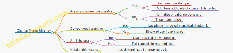
Practical Edge Cases That Affect Correctness
- Ties: Use deterministic tie-breaking (for example, by id) so pagination and retries don’t reshuffle results.
- Empty shards: Treat them as contributing no candidates; do not assume N lists are non-empty.
- Duplicate ids with different scores: Keep the maximum score if scores are comparable; otherwise keep the normalized maximum.
- Heap size smaller than k: Ensure you only stop early when the heap truly contains k items; otherwise you might stop too soon.
Top-k merging is where distributed retrieval either stays mathematically honest or quietly becomes “mostly right.” The good news: with heap merging, careful deduplication, and optional threshold stopping, you can keep both correctness and latency under control.
8.3 Score Normalization Across Shards and Index Variants
Distributed vector retrieval often returns partial top-k results from multiple shards, each using its own index variant and distance computation path. If you simply concatenate scores, the global ranking can be wrong because scores are not guaranteed to be on the same scale. Score normalization fixes this by mapping shard-local scores into a shared, comparable space.
Why Scores Drift Across Shards
Even when every shard stores the same embedding model, scores can differ due to:
- Different index families: one shard might use an HNSW-like graph, another might use IVF with quantization.
- Different quantization parameters: compressed distances can be systematically biased.
- Different filtering paths: some shards may apply metadata filters earlier, changing which candidates are even eligible.
- Different distance conventions: cosine similarity, inner product, and L2 distance produce different numeric ranges.
A practical rule: if two shards do not compute the same “raw score” definition end-to-end, you must normalize before merging.
Step 1: Standardize the Raw Score Definition
Before any normalization, enforce a consistent raw score across shards. For example, choose one of these canonical forms:
- Cosine similarity: normalize embeddings to unit length, then use inner product as cosine.
- L2 distance: keep L2 and convert to a similarity-like score by negating distance.
Example: if shard A returns inner product and shard B returns negative L2 distance, convert both into a single similarity score s where higher is better.
Step 2: Normalize Within Each Shard Using Calibration
A robust approach is to calibrate each shard’s scores using a small reference set and then apply an affine transform.
For each shard i, compute two parameters a_i and b_i so that:
s_norm = a_i * s_raw + b_i
How to get a_i and b_i without heroics:
- Sample a fixed set of queries.
- For each query, compute candidate scores from shard
i. - Compare shard-local scores to a reference baseline score computed by an exact or high-recall method on the same candidates.
- Fit
a_iandb_iusing least squares on the paired score values.
This makes shard score distributions align enough that top-k merging behaves consistently.
Step 3: Use Rank-Aware Normalization When Scales Still Differ
Affine calibration can fail when score distributions are non-linear, especially with heavy quantization. In that case, normalize using rank within the shard.
- Convert each candidate’s position
rin the shard’s ranked list into a monotonic score. - A simple mapping is
s_rank = -rors_rank = 1 / (r + 1).
This sacrifices some numeric fidelity but preserves ordering within each shard and prevents one shard from dominating purely due to scale.
Step 4: Merge Candidates with a Single Global Comparator
After normalization, merge candidates from all shards using the same comparator: higher normalized similarity wins.
Example: suppose you request global top-5.
- Shard 1 returns candidates with raw scores around
0.72to0.81. - Shard 2 returns raw scores around
12to18because it reports a different distance convention. - After canonical conversion and calibration, both sets map into a shared range, and the merge selects the truly best candidates.
Mind Map: Score Normalization Across Shards
Example: Two Shards with Different Index Variants
Assume both shards store the same vectors but:
- Shard A uses an uncompressed index and returns cosine similarity
sA. - Shard B uses quantization and returns an approximate inner product
sB.
At query time:
- Convert both to a canonical “higher is better” similarity.
- Apply shard calibration:
sA_norm = aA * sA + bAsB_norm = aB * sB + bB
- Merge all candidates and select global top-k by
s_norm.
If you skip step 2, shard B might look consistently better or worse depending on its quantization bias, and the global ranking will drift.
Determinism and Tie Breaking
When normalized scores tie, use a deterministic secondary key such as (doc_id, shard_id) order. This prevents “random-looking” changes between runs when two candidates are effectively equivalent after normalization.
Practical Checklist
- Confirm every shard reports a canonical raw score definition.
- Calibrate per shard when index variants differ.
- Use rank-aware normalization when calibration residuals are large.
- Merge with one comparator and deterministic tie breaking.
- Validate with offline evaluation using the same global top-k metric you care about.
8.4 Early Termination with Deterministic Bounds
Early termination stops a distributed top-k retrieval query before every shard finishes, but it must do so without changing the final answer set for a given snapshot. The trick is to compute a bound on what unseen work could still contribute, then stop only when that bound can’t beat the current top-k.
Core Idea: Bounds over Remaining Candidates
Assume each shard returns candidates in some order (for example, by increasing distance in an approximate index traversal). At any moment, you have:
- Current top-k across all shards, with a threshold score
T(the k-th best score so far). - Per-shard remaining bound
B_sthat upper-bounds the best score any unseen candidate on shardscould still achieve.
If for all shards s, B_s <= T, then no future candidate can enter the global top-k. You can stop fanout and merging immediately.
This is deterministic when:
- The bound computation is deterministic for the same index snapshot.
- Tie-breaking is deterministic (for equal scores, use a stable secondary key like
(score, doc_id)with doc_id ascending).
Deterministic Tie Breaking and Score Conventions
Bounds depend on score direction. For cosine similarity, higher is better; for distance, lower is better. Pick one convention and stick to it.
A practical convention for similarity search:
- Use higher-is-better scores.
- Maintain top-k by
(score desc, doc_id asc). - Define
Tas the score of the current k-th element, and if the k-th element has ties, include the tie-breaking rule when comparing against bounds.
When comparing B_s to T, treat equality carefully: if B_s == T, you still might need more candidates if they could match T with a smaller doc_id. The simplest deterministic approach is to store not only T but also the current k-th doc_id under the tie-break ordering, and compare (score, doc_id) pairs.
How Per-Shard Bounds Are Computed
Bounds come from properties of the traversal order and index structure.
Common patterns:
- Distance-ordered traversal: if the shard explores candidates in non-increasing score order, then the best unseen candidate cannot exceed the next frontier’s best possible score. The bound can be derived from the priority queue key.
- Quantized or compressed scoring: if approximate distances are refined in stages, the bound can be the best possible score after the remaining refinement steps. For example, if you have a coarse quantized score and a known maximum correction range, you can bound the refined score.
- Graph-based search: if the algorithm maintains a candidate priority and only expands nodes whose potential exceeds the current threshold, the bound is the maximum potential of the unexpanded queue.
The key requirement is monotonicity: as you process more, bounds should not get looser.
Mind Map: Early Termination with Deterministic Bounds
Example: Three Shards and a Safe Stop
Suppose you query for top-3 by cosine similarity. Scores are higher-is-better, and ties break by smaller doc_id.
- Initial global top-3 is empty, so
T = -∞. - Shard 1 explores candidates and finds:
(0.91, doc 10),(0.88, doc 7),(0.86, doc 3). Now global top-3 is these three, soT = 0.86andkthDocId = 3. - Shard 2 has not finished. Its traversal maintains a frontier bound
B2 = 0.85for any unseen candidate. Since0.85 < 0.86, shard 2 can’t beat the threshold. - Shard 3 is still working, but its frontier bound is
B3 = 0.86. Because equality is possible, you must compare tie-break pairs. The best unseen candidate on shard 3 could only reach score0.86, but its bound also implies the smallest possible doc_id among unseen candidates isdoc 20(from how the index orders candidates). The pair(0.86, 20)is worse than(0.86, 3), so it can’t enter the top-3.
Now all shards satisfy the stop condition: shard 1 is already processed enough to define the threshold, shard 2 is strictly below, and shard 3 is equal but worse under tie-break. You stop immediately, even though shard 3 still has queued work.
Implementation Checklist for Correctness
- Maintain top-k as
(score, doc_id)pairs. - Track
TandkthDocIdfrom the current global top-k. - For each shard, expose a deterministic
Bsderived from its traversal frontier or remaining refinement stage. - Stop only when every shard’s bound is not better than
(T, kthDocId)under the same ordering. - Ensure the index snapshot and traversal order are consistent across retries so the bound logic matches the actual candidate space.
Done right, early termination reduces wasted work while keeping the result stable and reproducible for the same dataset and query.
8.5 Handling Pagination and Stable Ranking Under Updates
Pagination sounds simple until updates arrive mid-session. If you page through results while documents are being inserted, deleted, or re-embedded, the same item can appear twice, disappear, or jump positions. Stable ranking means that for a given user session and query, the relative order of results remains consistent even as the underlying index changes.
Core Idea: Snapshot Semantics for a Session
A practical approach is to pin a logical snapshot at the start of the pagination flow. Each request carries a session_token that identifies the snapshot boundary. The system then answers all pages using the same snapshot view.
- Without snapshotting: page 1 might include an item that gets deleted before page 2, causing fewer than
kresults and shifting ranks. - With snapshotting: page 2 sees the same candidate set as page 1, so pagination is deterministic.
A snapshot can be implemented as a combination of index versioning and visibility rules. For example, each shard maintains an index build id and a visibility watermark; queries filter out documents newer than the watermark.
Deterministic Tie Breaking for Equal Scores
Even with snapshot semantics, ties happen when scores match due to quantization, rounding, or identical similarity values. Stable ranking requires a deterministic secondary sort key.
Use a strict ordering like:
- primary: descending similarity score
- secondary: descending shard-local document timestamp or ingestion sequence
- tertiary: ascending
doc_id(unique and immutable)
This prevents “random” ordering when multiple documents share the same score.
Pagination Strategy: Cursor-Based over Offset-Based
Offset-based pagination (offset = page * size) is fragile under updates because the “window” moves. Cursor-based pagination uses the last item from the previous page as an anchor.
A cursor typically includes:
- the snapshot token
- the last item’s score
- the last item’s tie-break fields (e.g.,
seq,doc_id)
Then the next page requests results strictly “after” that cursor in the deterministic order.
Example: Cursor Fields and Next-Page Filter
Suppose results are ordered by (score desc, seq desc, doc_id asc). If the last item on page 1 is (0.7421, seq=105, doc_id=abc), then page 2 returns items where:
- score < 0.7421, or
- score = 0.7421 and seq < 105, or
- score = 0.7421 and seq = 105 and doc_id > abc
This logic is simple, but it must be applied consistently across shards and after result merging.
Mind Map: Stable Pagination Under Updates
Distributed Retrieval: Where Stability Can Break
Stability often fails during merging. Each shard returns its local top candidates; if you apply cursor filtering only after merging, you may still fetch too few items to fill the page. Conversely, if you apply cursor filtering too early without consistent ordering keys, you can skip valid candidates.
A robust pattern is:
- Each shard returns candidates sorted by the global ordering keys.
- The coordinator merges using the same comparator.
- The coordinator applies the cursor predicate during merge and continues pulling from shards until the page is filled.
This ensures that pagination boundaries are respected globally, not just locally.
Example: Comparator and Cursor Predicate
Global order comparator
- higher score first
- if score equal: higher seq first
- if seq equal: lower doc_id first

Cursor predicate for next page
- (score < last.score)
  OR (score == last.score AND seq < last.seq)
  OR (score == last.score AND seq == last.seq AND doc_id > last.doc_id)
Handling Updates Without Surprises
Treat updates as versioned changes. When a document is re-embedded, store it as a new version with a new seq, and mark the old version as superseded. Snapshot queries see either the old or new version depending on the watermark.
Deletes follow the same rule: a delete creates a tombstone version. Snapshot queries exclude documents whose tombstone is visible under the snapshot token.
Practical Checklist
- Use cursor-based pagination with a deterministic tie-break comparator.
- Pin a snapshot token for the entire pagination session.
- Apply the cursor predicate during distributed merge to guarantee page size.
- Version documents and tombstones so snapshot visibility is consistent.
- Ensure all shards use identical ordering keys and numeric rounding rules.
When these pieces align, pagination becomes boring in the best way: the user sees the same ordered list across pages, even while the index keeps changing in the background.
9. Hybrid Retrieval with Metadata Filters and Reranking
9.1 Metadata Indexing with Inverted Indexes and Column Stores
Vector search rarely lives alone. In practice, you almost always need metadata constraints like tenant_id, language, doc_type, or time ranges. The goal of metadata indexing is simple: reduce the candidate set before you touch the vector index, and do it with predictable latency.
Core Idea: Candidate Filtering Before Vector Scoring
A typical two-stage flow looks like this:
- Parse the query and extract filter predicates.
- Use metadata indexes to produce a candidate document ID set.
- Run vector similarity only on those candidates.
- Optionally rerank using additional signals.
The tricky part is step 2. If you filter poorly, you either scan too many vectors or you miss valid matches.
Metadata Types and What Index They Need
Metadata fields fall into a few common buckets:
- Exact match:
tenant_id=acme,language=en. - Low-cardinality enums:
doc_type=policy|manual. - Multi-valued tags:
tags contains {security, oauth}. - Range filters:
timestamp between t1 and t2. - Optional fields: missing values should behave consistently.
Inverted indexes handle exact and multi-valued fields well. Column stores handle range scans and aggregations efficiently when you can narrow by row groups.
Inverted Indexes for Exact and Multi-Valued Filters
An inverted index maps term → postings list. For metadata, the “term” is usually a normalized token.
Example:
- Field:
tags - Document 101 has
tags=[security, oauth] - Document 205 has
tags=[security, pii]
Then:
security → [101, 205, ...]oauth → [101, ...]
For a query tags contains security AND oauth, you intersect postings lists: security ∩ oauth.
Best practices that keep this fast:
- Use sorted postings lists so intersection is linear in the smaller list.
- Store doc IDs as integers and compress them (delta encoding) to reduce memory bandwidth.
- Normalize terms consistently (case folding, trimming, canonical enum values).
Column Stores for Range Filters and Efficient Row Pruning
A column store keeps each field in a separate contiguous layout. That makes it easy to apply range predicates without touching unrelated fields.
For timestamp, you can store values in sorted order within row groups (or keep min/max per block). Then a filter like timestamp >= 2026-02-20 can skip entire blocks whose max is too small.
A practical pattern:
- Maintain min/max per block for range fields.
- When a query arrives, compute which blocks can contain matches.
- Produce candidate doc IDs from only those blocks.
Combining Inverted Indexes and Column Stores
When filters include both exact terms and ranges, you want a deterministic order:
- Use inverted indexes for the most selective exact predicates.
- Use column-store pruning for range predicates.
- Intersect the resulting candidate sets.
Selection order matters because intersection cost depends on candidate set sizes. A good heuristic is “smallest first,” based on postings list lengths and block selectivity.
Mind Map: Metadata Indexing Strategy
Example: Filtered Candidate Generation
Suppose you have:
tenant_idexact matchlanguageexact matchtimestamprangetagsmulti-valued
Query:
tenant_id=acmelanguage=entimestamp between 2026-02-20 and 2026-03-01tags contains security AND oauth
Execution:
- Get postings for
tenant_id=acmeand intersect withlanguage=en. - Intersect with
tags securityand thentags oauth. - Apply the timestamp range using column-store block pruning to get a doc ID set.
- Intersect the timestamp set with the current candidate set.
- Run vector search only on the final candidate IDs.
This ordering avoids scanning vectors for documents that fail cheap metadata checks.
Practical Implementation Notes
- Doc ID Set Representation: use sorted arrays for small sets; switch to bitsets for dense sets.
- Short-Circuiting: if any predicate yields an empty set, stop immediately.
- Stable Semantics for Missing Values: decide whether missing fields mean “no match” or “match only when explicitly requested.”
Mind Map: Filter Execution Plan

Summary of the Integration
Inverted indexes give you fast exact and tag filtering through postings intersections. Column stores give you efficient range pruning through block-level statistics. When you combine them with a selectivity-aware execution plan, you shrink the candidate set early and keep vector retrieval focused on the documents that actually have a chance to score well.
9.2 Filter Pushdown Techniques with Vector Indexes
Filter pushdown means applying metadata constraints as early as possible, so the vector index searches fewer candidates. The goal is simple: reduce wasted distance computations while keeping ranking correct for the filtered set. The tricky part is that “filtered set” is not the same as “filtered candidates,” because approximate indexes may skip items that would have matched under a strict brute-force filter.
Foundational Model of Filtered Retrieval
Assume each item has:
- A vector embedding used for similarity.
- Metadata fields such as
tenant_id,doc_type,language, andtimestamp. - A query embedding plus optional filter predicates.
A correct system returns the top k items by similarity among items satisfying the predicates. Filter pushdown tries to enforce predicates before or during the vector search, rather than after retrieving an unfiltered candidate pool.
A practical way to reason about correctness is to separate two stages:
- Candidate generation using the vector index.
- Candidate validation and reranking using exact predicate checks.
Pushdown improves stage 1 efficiency; stage 2 preserves correctness.
Mind Map: Where Filters Enter the Pipeline
Filter Pushdown Mind Map
Equality Filters with Partition-Aware Indexing
If a filter is an equality on a high-cardinality field like tenant_id, the cleanest pushdown is to partition data by that field. Then the vector index only exists within each partition. For example, if a query includes tenant_id=acme, you route the request to the acme shard and search its index. This avoids scanning other tenants entirely.
A common pitfall is assuming partitioning alone guarantees correctness when you also use approximate search. It does, as long as the index contains only items from the partition and the query is routed accordingly. The approximate nature affects recall within the partition, not whether items from other tenants leak in.
Range Filters with Segmenting and Cluster Pruning
Range filters like timestamp >= 2026-02-01 are harder because they don’t map to a single key. A reliable approach is to segment the index by time windows (for example, monthly segments). At query time, you select the segments that could contain matches, then run vector search only inside those segments.
If you use an IVF-style index, you can add another layer: cluster pruning. Maintain lightweight postings that record which clusters contain vectors from each segment. When the query selects segments, you probe only clusters marked as present for those segments. This reduces the number of probed centroids and the number of candidate vectors that need distance computations.
Set Membership Filters with Inverted Metadata Indexes
For filters like doc_type IN {spec, report}, build an inverted index mapping each doc_type value to the set of vector IDs (or to bitsets per segment). Pushdown then becomes: compute the union of ID sets for the requested types, and restrict vector search to those IDs.
In practice, you rarely want to restrict every distance computation to an arbitrary ID set, because that can turn a fast index traversal into a slow membership test. A better pattern is to convert the ID set into segment-local bitsets, then use them to:
- Gate candidate acceptance during traversal.
- Stop early when the remaining candidate budget in a segment is exhausted.
Graph-Based Index Traversal Constraints
For HNSW-like graphs, pushdown can be applied during neighbor expansion. Suppose you have a filter language=en. You can mark nodes (or underlying items) with language. During traversal, you only consider neighbors whose items satisfy the predicate.
This is efficient when the predicate is selective and when the graph traversal already touches only a small neighborhood. It can be less efficient when the predicate is broad, because you still pay traversal overhead but gain little pruning.
Correctness requires that the traversal’s candidate set is large enough to compensate for the filter-induced pruning. If you set the traversal budget too low, you may miss valid top-k items even though all predicate checks are correct.
Candidate Budgeting and Early Termination
Filter pushdown changes the effective candidate pool size. A robust engineering rule is to treat the vector index’s ef-like parameter (or probe count) as a function of filter selectivity.
Example: if an unfiltered query typically examines 50,000 candidates to achieve stable recall, a filter that keeps 5% of items might examine 2,500 candidates instead of 50,000. The exact numbers depend on the index, but the principle holds: keep enough candidates so that approximate skipping doesn’t dominate.
Early termination should also respect filtering. If you maintain a running best-so-far similarity threshold, you can stop when the maximum possible score for any not-yet-explored candidate cannot beat the threshold. With filters, “not-yet-explored” must mean “not-yet-explored among predicate-satisfying items,” not just “not-yet-explored in the index.”
Example: Filter Pushdown with IVF Probing and Post-Validation
Consider an IVF index with 1024 clusters. Each cluster stores centroid assignments, and you keep a cluster-to-segment presence map.
Query:
- Similarity: cosine
- Filter:
tenant_id=acmeandtimestamp >= 2026-02-01
Steps:
- Route to the
acmepartition. - Select time segments starting at 2026-02-01.
- From the presence map, determine which clusters exist in those segments.
- Probe only those clusters, generate candidates, and compute exact cosine similarity.
- Validate predicates exactly on each candidate before inserting into the top-
kheap.
This pipeline avoids scanning vectors from other tenants, avoids probing clusters that cannot contain matching time segments, and still guarantees correctness because predicate checks happen on the final candidate set.
Mind Map: Practical Pushdown Checklist
Filter pushdown works best when it reduces the search space in a way that matches how the index organizes data. When that alignment is missing, the system still benefits from pruning, but it must compensate with careful candidate budgeting and exact predicate validation.
9.3 Two Stage Retrieval with Candidate Generation and Reranking
Two stage retrieval keeps the fast part fast and the accurate part accurate. Stage one generates a small set of candidates using a vector index and cheap scoring. Stage two reranks those candidates using a stronger model or richer features, then returns the final top k.
Stage One Candidate Generation
Stage one answers: “Which documents are even worth considering?” It typically uses an ANN vector index plus optional metadata filters.
Core steps
- Embed the query into the same vector space as the documents.
- Apply metadata filters early when possible, so the index searches only relevant shards or partitions.
- Retrieve top n candidates by approximate similarity, where n is larger than the final k (for example, n=200 when k=10).
- Optionally include a lightweight lexical signal by mixing scores from a text index and the vector index.
Practical example Suppose a support assistant searches for “reset password for SSO account.” The vector index might return 200 candidates that are semantically close, including articles about “SSO login issues,” “account access,” and “authentication failures.” Even if some are off by a detail, they are likely to contain the right section somewhere.
Why n matters If n is too small, the reranker never sees the correct document. If n is too large, reranking becomes expensive and latency grows. A common starting point is n=20 to 200 depending on reranker cost and acceptable tail latency.
Stage Two Reranking
Stage two answers: “Given these candidates, which ones should win?” Reranking uses a more expressive scoring function that can consider query-document interactions.
Common reranking inputs
- Query text and document title
- Document snippet or passage
- Structured fields such as category, language, or product
- Optional cross features like overlap counts or field-specific similarity
Reranker scoring patterns
- Cross encoder style scoring that reads query and candidate together
- Bi-encoder reranking where candidates are re-embedded with a different model
- Feature-based scoring that combines vector similarity with metadata rules
Example reranking logic For each candidate, compute:
- semantic_score from the vector similarity
- filter_score from metadata match quality
- interaction_score from a cross-encoder or feature overlap Then combine them into a single rank score, for example:
- rank_score = 0.6 * interaction_score + 0.3 * semantic_score + 0.1 * filter_score
This weighting is not magic; it is tuned on labeled queries so the reranker learns what “good” looks like for your domain.
Score Calibration and Stable Ordering
Stage one and stage two often produce scores on different scales. Reranking should not assume stage one similarity is comparable to reranker outputs.
Best practices
- Use reranker score as the primary ordering key.
- If you combine scores, normalize each component using statistics from a validation set.
- Add deterministic tie breaking, such as sorting by document id when scores match.
Concrete pitfall If you simply add raw cosine similarity to a cross-encoder logit, the cosine term can dominate because it has a larger numeric range. Normalization prevents that kind of silent failure.
End-to-End Flow
The integrated flow below shows how candidate generation and reranking fit together.
Input: query q, filters F, final k, candidate size n
1) vq = Embed(q)
2) C = ANN_Search(index, vq, filters=F, top_n=n)
3) For each doc d in C:
     features = BuildFeatures(q, d)
     s2[d] = RerankScore(features)
4) Sort C by s2 descending, tie-break by doc_id
5) Return top k documents with scores and explanations
Mind Map: Two Stage Retrieval
Example: Measuring Reranker Hit Rate
A simple metric checks whether the reranker has a chance to succeed.
- Define “hit” as: the ground-truth document appears in the candidate set C.
- Compute hit@k_candidate for candidate size n.
If hit rate is low, increasing n or improving stage one filtering usually helps more than changing reranker weights.
Example: Candidate Size Tuning
Assume k=10 and you observe:
- n=50 gives hit rate 0.72
- n=100 gives hit rate 0.86
- n=200 gives hit rate 0.90
If reranking latency is acceptable at n=100 but not at n=200, choose n=100. The goal is not maximum recall; it is the best tradeoff that keeps the system responsive while giving the reranker enough candidates to work with.
9.4 Cross Encoder and Bi Encoder Reranking Integration Patterns
Reranking usually means: generate a small candidate set with a fast bi-encoder style retriever, then score those candidates with a slower cross encoder that can look at the query and candidate together. The integration patterns below focus on how to pass data, how to keep latency predictable, and how to avoid subtle ranking inconsistencies.
Mind Map: Reranking Integration Patterns
Pattern 1: Two Stage Retrieval with Deterministic Candidate Payloads
Start with a bi-encoder retriever that returns top_k candidates plus stable identifiers. Then build cross-encoder inputs using a deterministic template so the same query-candidate pair always produces the same token sequence.
Example: Suppose each document has title, body, and category. Your candidate payload should include exactly the fields you will feed the cross encoder. If you decide to score using title + body, then always concatenate in that order and apply the same truncation boundary (for instance, keep the full title and truncate body to a fixed token budget).
Best practice: Store a “reranker view” of each document at ingestion time, such as rerank_text = title + "\n" + body. This avoids runtime field assembly differences and reduces CPU overhead during query serving.
Pattern 2: Filter Aware Candidate Generation with Reranker Consistency
If you apply metadata filters (like category = support), apply them before candidate generation so the cross encoder never sees candidates that would be excluded anyway. This keeps the reranker’s work aligned with the user-visible result set.
Example: Query asks for “reset password”. If the user requests only category = account, ensure the bi-encoder retrieval is executed within that filtered subset. Then the cross encoder reranks only those candidates. Otherwise, you can end up with a top candidate that would have been filtered out, and you’ll waste compute while also complicating debugging.
Pattern 3: Batch Reranking with Latency Budgeting
Cross encoders are expensive because they run attention over query-candidate pairs. To keep latency stable, batch reranking across queries when possible, and cap the number of candidates per query.
Example: If your service budget allows 40 ms for reranking, you might choose top_k = 50 and run cross-encoder inference in batches of 16 pairs. If the batch is not full, you still run it after a short wait window to avoid tail latency spikes.
Best practice: Use a fixed maximum candidate count per query. If the retriever returns fewer than top_k after filters, rerank only what you have and keep the output schema consistent.
Pattern 4: Score Calibration and Stable Ordering
Cross encoders often output logits that are not directly comparable across queries. You typically only need ordering within a query, but you still want stable results when scores are equal or nearly equal.
Example: If two candidates receive the same reranker score due to rounding, break ties using the bi-encoder similarity score, then by document id. This prevents “random-looking” changes between runs.
Best practice: Apply a per-query normalization step only if your downstream logic expects bounded scores. Otherwise, keep raw reranker scores and use deterministic tie-breaking.
Pattern 5: Partial Rerank and Fallback Behavior
Reranking can fail for a subset of candidates due to malformed text, missing fields, or transient model issues. Decide how the system behaves so users get consistent results.
Example: If 3 out of 50 candidates cannot be tokenized, rerank the remaining 47 and place the failed ones at the bottom using their bi-encoder scores. If the cross encoder fails entirely, return the bi-encoder top-k with no reranking.
Best practice: Log which candidates were excluded from reranking and why, but do not change the output ordering rules between failure modes.
Pattern 6: Training Alignment with Inference Inputs
The cross encoder learns from the exact input format it sees during training. If inference concatenates fields differently than training, ranking quality drops in ways that are hard to diagnose.
Example: Training might use [query] [SEP] [title] [SEP] [body] while inference uses title + "\n" + body without separators. Keep the same structure, including separators and truncation strategy.
Best practice: Generate hard negatives using the bi-encoder retriever so the cross encoder learns to correct the retriever’s typical mistakes. This makes reranking do useful work instead of re-deriving obvious distinctions.
Mind Map: Practical Integration Checklist
Example: End-to-End Flow for One Query
- Bi-encoder retrieves top 50 candidates within the requested filter.
- Service builds reranker inputs using the precomputed
rerank_textfor each candidate. - Cross encoder scores all pairs in one or more batches.
- Candidates are sorted by cross-encoder score, with ties broken by bi-encoder score then document id.
- If tokenization fails for a candidate, it is assigned a fallback rank position using bi-encoder score.
This structure keeps reranking focused, predictable, and explainable: the retriever narrows the search space, the cross encoder corrects ranking within that space, and the system rules make behavior consistent even when things go wrong.
9.5 Ensuring Reproducible Ranking with Deterministic Tie Breaking
Reproducible ranking means the same inputs produce the same ordered results, even when multiple candidates have equal scores. In vector search, ties happen more often than people expect: quantization can collapse distances, floating-point math can round differently across hardware, and distributed merging can reorder equal-score candidates.
What Causes Ties in Practice
- Equal similarity values: Two vectors can yield the same cosine similarity after normalization or compression.
- Quantization collisions: Product quantization can map different vectors to the same code, producing identical approximate distances.
- Floating-point non-determinism: Parallel reductions and SIMD paths can change the last bits.
- Distributed partial results: Shards may return candidates with equal scores, and the merge step can pick different winners if it doesn’t define a stable ordering.
A deterministic tie breaker turns “equal score” into “ordered by rule,” so the system behaves like a well-mannered librarian: same book, same shelf.
Deterministic Ordering Strategy
Use a lexicographic sort key that is identical across all nodes:
- Primary key: score (descending for similarity, ascending for distance)
- Secondary key: document identifier (ascending)
- Tertiary key: optional stable sub-identifier (chunk id, version id)
If you rerank, apply the same rule to the reranked list. If reranking changes scores, ties can still occur, so the tie breaker must remain in place.
Mind Map: Deterministic Ranking Pipeline
Score Normalization Without Breaking Determinism
When merging shard results, you often normalize scores so that “bigger is better” holds everywhere. Determinism requires that normalization be identical across shards and runs.
- Use the same formula everywhere (no per-shard min/max scaling unless it’s computed deterministically from the same dataset snapshot).
- If you must scale, compute scaling constants from stored metadata or from a fixed configuration, not from runtime statistics that can vary.
A simple rule: normalization should be a pure function of (raw_score, metric_config).
Distributed Merge with Stable Top-k
A common failure mode is using an unstable heap or sorting without a secondary key. The fix is to merge using the deterministic sort key.
Example merge rule for similarity (higher is better):
- Candidate A beats B if:
scoreA > scoreB, orscoreA == scoreBanddoc_idA < doc_idB, orscoreA == scoreBanddoc_idA == doc_idBandchunk_idA < chunk_idB.
This rule must be applied consistently during:
- shard-level top-k selection
- global top-k selection
- deduplication when the same document appears from multiple shards
Example: Tie Break in a Two-Shard Merge
Assume k=3 and both shards return candidates with identical scores:
- Shard 1 returns: (score 0.812, doc 42), (score 0.812, doc 7), (score 0.801, doc 9)
- Shard 2 returns: (score 0.812, doc 7), (score 0.812, doc 13), (score 0.799, doc 5)
After dedup by (doc_id, chunk_id) and sorting by (score desc, doc_id asc, chunk_id asc), the top three become:
- (0.812, doc 7)
- (0.812, doc 13)
- (0.812, doc 42)
Without the secondary key, the order among doc 7, 13, and 42 could flip depending on arrival order.
Testing for Reproducibility
Reproducibility tests should be strict and boring:
- Same request, same output: Run the same query multiple times on the same cluster and compare the full ordered list of
(doc_id, chunk_id). - Cross-node consistency: Route the query to different shard subsets (or vary concurrency) and confirm identical ordering.
- Tie-heavy fixtures: Use a small dataset where many vectors quantize to the same codes, forcing ties.
A good test asserts equality of the final ranked list, not just the set of documents.
Practical Checklist
- Define a deterministic sort key and use it in every stage that orders candidates.
- Ensure deduplication preserves the canonical identity used by the tie breaker.
- Make score normalization a pure, identical function across shards.
- Reapply tie breaking after reranking.
- Add tests that intentionally create ties.
Deterministic tie breaking is less about fancy math and more about refusing to let “equal” mean “random.”
10. Performance Engineering for Latency Throughput and Cost
10.1 Profiling End to End Latency with Traceable Components
End-to-end latency is what users feel, but it’s also what engineers need to explain. The goal of profiling is not just to measure a number; it’s to produce a timeline where each segment has a name, a unit, and a way to reproduce it. A practical approach starts with a traceable component map, then adds instrumentation, then validates that the measurements match reality.
Mind Map: Traceable Latency Components
Step 1: Define Span Boundaries That Match Reality
Start by deciding where a span begins and ends. A good rule is: a span boundary should correspond to a single responsibility and a measurable action. For example, “Query Preparation” should include embedding retrieval and vector normalization, but it should not include “Shard fanout,” because those are separate systems with different failure modes.
A minimal span set for a vector search request:
client_request: client serialization and HTTP/gRPC sendapi_gateway: auth, validation, routingembedding: lookup or generationfanout: dispatch to shardsshard_search: per-shard index search and candidate collectionmerge_topk: merging partial resultsrerank: optional reranking inferenceresponse_assemble: formatting and compressionclient_response: receive and deserialize
Step 2: Instrument with Consistent Timing Units
Use monotonic clocks for durations and record both wall time and CPU time when possible. Wall time tells you what users wait for; CPU time tells you whether the system is busy or just waiting on queues.
For each span, capture:
- duration in milliseconds
- status (success, timeout, error)
- cardinality-safe tags (collection, index version, request type)
- queue time if the component has an internal queue
A common mistake is measuring only “search time” and ignoring queueing. If your p95 latency is dominated by queueing, tuning the index won’t help until you fix admission control.
Step 3: Validate Instrumentation with a Controlled Example
Use a single request with known inputs and run it under load that matches production concurrency. Then compare:
- trace timeline sum of spans vs. end-to-end measured latency
- per-shard search duration vs. total retrieval duration
- merge time vs. number of candidates returned
If the sums don’t match, you likely have gaps: uninstrumented work, time spent in middleware, or retries that reuse the same trace ID without adding spans.
Example: Interpreting a Trace Timeline
Suppose a request shows:
fanout: 8 msshard_search: 42 ms average across 6 shardsmerge_topk: 6 msrerank: 55 msresponse_assemble: 3 ms
The end-to-end latency is about 114 ms plus network overhead. Here, reranking dominates. If you remove reranking, you should see the p95 drop roughly by the rerank span duration. If it doesn’t, then reranking might be blocked on batching, or the system might be queueing earlier than you think.
Step 4: Add Queueing Visibility and Backpressure Clues
For components that can queue (API workers, shard request handlers, rerank batching), record:
- time in queue
- time executing
- queue length at dispatch
When p99 spikes, check whether queue time grows while execution time stays flat. That pattern points to overload or admission issues. If both queue and execution grow, you may have contention (CPU saturation, GC pressure, or memory bandwidth limits).
Step 5: Turn Traces into Actionable Metrics
Traces answer “why this request was slow.” Metrics answer “how often and where.” For each span, publish percentiles and error rates. At minimum:
- p95 and p99 for
fanout,shard_search,merge_topk, andrerank - timeout counts by component
- retry counts by component
Finally, correlate spikes with index version and model version tags. If a new index build changes traversal behavior, you’ll see shard_search shift without touching embedding or merge logic.
Mind Map: Profiling Workflow
A traceable profiling setup makes latency engineering less guessy. You can point to a specific span, quantify its contribution, and then change the smallest thing that can plausibly move that span.
10.2 Batch Querying and Concurrency Control Mechanisms
Batch querying means sending multiple retrieval requests together so the system can reuse work and keep hardware busy. Concurrency control means deciding how many requests run at once, and how they share CPU, memory, and network without turning latency into a lottery.
Core Concepts That Make Batching Work
A vector retrieval request typically has three stages: embedding lookup or generation, candidate retrieval from an index, and optional reranking or filtering. Batching helps most when stages can share overhead.
- Shared overhead: If you already have query embeddings, batching avoids repeated request parsing, network round trips, and per-request thread scheduling.
- Vectorized compute: Many distance computations can run faster when you process multiple query vectors together, especially on CPUs with SIMD and on GPUs with larger matrix operations.
- Predictable resource use: Instead of letting each request independently allocate buffers, you can pre-size batch buffers and reuse them.
A practical rule: batch size should be chosen based on the slowest stage. If reranking dominates, batching candidates may help less than batching retrieval.
Batch Shapes and Scheduling
Batching is not just “more queries at once.” You need a batch shape that matches your pipeline.
- Fixed batch size: Simple and stable, but may add waiting time while you wait to fill the batch.
- Time-window batching: Collect requests for a short window (for example, 5–20 ms) and then dispatch whatever you have.
- Dynamic batching: Choose batch size based on current load and observed compute time.
To keep latency bounded, use a queue with two controls: a maximum wait time and a maximum batch size. If either limit triggers, dispatch the batch.
Concurrency Control That Prevents Queue Collapse
Concurrency control is about limiting in-flight work. Without it, queues grow, memory spikes, and tail latency explodes.
Use a layered approach:
- Admission control: Cap the number of requests accepted per service instance.
- Per-stage limits: Limit concurrency separately for embedding generation, index search, and reranking.
- Backpressure: When a stage is saturated, stop accepting new work or route to a degraded mode that still returns correct results.
A simple mental model: each stage has a “service rate.” If you let arrival rate exceed service rate, the queue grows without bound. Concurrency limits keep arrival rate within what the slowest stage can handle.
Mind Map: Batch Querying and Concurrency Control
Example: Time-Window Batching with Bounded Latency
Suppose you run an index search service that can process 64 query vectors per compute call efficiently. You also want to avoid waiting too long.
- Set max batch size to 64.
- Set max wait time to 10 ms.
- If fewer than 64 requests arrive within 10 ms, dispatch the partial batch.
This keeps latency predictable: fast streams get small batches, while busy periods get full batches.
Example: Per-Stage Concurrency Limits
Imagine a pipeline where embedding generation is slower than index search.
- Embedding stage: allow 16 concurrent embedding jobs.
- Index search stage: allow 64 concurrent search batches.
- Reranking stage: allow 8 concurrent rerank jobs.
If reranking is optional, you can also treat it as a separate queue with its own cap. That way, reranking saturation does not block retrieval for requests that only need candidates.
Example: Queueing and Timeouts in Practice
A robust pattern is to attach a deadline to each request and enforce it at each stage.
- If the request reaches the index stage after its deadline, skip reranking and return candidates only.
- If the request cannot be admitted due to in-flight caps, return a clear error or a cached response if available.
This keeps the system honest: it fails fast when overloaded instead of grinding through work that can no longer be delivered.
Implementation Sketch for a Batch Dispatcher
Below is a minimal dispatcher pattern. It uses a queue, a timer, and a batch cap.
queue = new RequestQueue()
maxBatch = 64
maxWaitMs = 10

function submit(req):
  queue.push(req)
  signalDispatcher()

function dispatcherLoop():
  while running:
    batch = []
    start = now()
    while batch.size < maxBatch and (now()-start) < maxWaitMs:
      req = queue.tryPop()
      if req == null: break
      batch.push(req)
    if batch.size > 0:
      runIndexSearch(batch)
This dispatcher is only half the story; you still need per-stage concurrency caps around runIndexSearch and any reranking stage so that one hot stage cannot starve others.
Tuning Checklist That Avoids Guesswork
- Measure stage latencies under load and identify the bottleneck stage.
- Choose batch size to improve the bottleneck stage, not the fastest one.
- Set max wait time so batching does not dominate end-to-end latency.
- Apply per-stage concurrency caps and enforce request deadlines.
- Validate with load tests that include bursty arrivals, not just steady traffic.
Batching and concurrency control work best when they are treated as two knobs on the same machine: batching improves efficiency, and concurrency limits keep the system from turning efficiency into backlog.
10.3 Hardware Considerations for CPU GPU and Memory Bandwidth
Vector retrieval performance is often limited less by “how fast the math is” and more by how quickly the system can move vectors, codes, and partial scores through caches and memory. The practical goal is to match your index layout and execution strategy to the bottlenecks of the hardware you actually run.
Start with the Bottleneck Model
Think in terms of three stages: (1) fetching candidate representations, (2) computing distances or similarity, and (3) updating top-k state. For many CPU deployments, stage (1) dominates because vectors are large and access patterns are irregular. For GPU deployments, stage (2) can be fast, but stage (1) still matters because global memory bandwidth and memory coalescing decide whether kernels spend time waiting.
A quick sanity check: if your per-vector compute is small (common with quantized codes), then doubling FLOPS won’t help much; you need better locality, fewer bytes per candidate, and fewer random reads.
CPU Hardware: Cache Lines, Prefetching, and SIMD
On CPUs, distance computation is usually SIMD-friendly, but only if data is laid out contiguously and accessed predictably. Store vectors in a structure-of-arrays layout when possible, so each SIMD lane reads contiguous elements. For quantized representations, keep codebooks and codes in separate, aligned buffers to reduce cache thrashing.
Top-k maintenance also affects bandwidth. If you keep a small heap per query in registers or L1, you avoid frequent writes to memory. A common pattern is to accumulate partial scores in a fixed-size array and only materialize the final top-k after processing a block of candidates.
Example: Suppose you store 768-d float vectors. A single vector is ~3 KB. If you scan 10,000 candidates, you read ~30 MB per query just for raw vectors, before any metadata. If instead you store 8-bit product-quantization codes, the candidate representation might be a few hundred bytes, cutting memory traffic by an order of magnitude.
GPU Hardware: Kernel Shape and Memory Coalescing
GPUs excel when you can batch many distance computations and keep threads busy. The key is to ensure that threads in a warp read adjacent bytes. That means your codes should be stored so that consecutive candidates map to consecutive memory addresses.
Avoid designs where each thread follows a different pointer chain into memory. If your index traversal produces irregular candidate sets, consider a two-step approach: first gather candidate IDs into a contiguous buffer, then run a dense distance kernel over that buffer.
Example: If you have per-shard candidate lists, first concatenate them into a single array of codes and offsets, then launch one kernel per query batch. This turns scattered reads into coalesced reads and reduces wasted bandwidth.
Memory Bandwidth: Bytes per Candidate as the Real Metric
Measure or estimate “bytes per candidate” end-to-end: representation bytes plus any additional reads for norms, metadata, or intermediate buffers. Then multiply by candidates examined per query. This gives a bandwidth demand you can compare to your system’s sustainable throughput.
A practical engineering tactic is to reduce bytes per candidate before tuning compute. Quantization and compression help, but so do execution choices like filtering earlier, using smaller candidate pools, and reusing cached query-side data.
Mind Map: Hardware Factors for Vector Retrieval
Integrated Example: Choosing CPU vs GPU Execution
Assume you run 1,000 queries per second with k=10. On CPU, you might examine 50,000 candidates per query with float vectors, which is enormous memory traffic. On GPU, you can examine fewer candidates because you can afford a larger batch and run a dense scoring kernel efficiently, but only if candidate codes are stored contiguously.
If your index uses quantized codes, both CPU and GPU benefit, but the CPU may still win when candidate sets are small and latency matters. The GPU tends to win when you can batch enough queries to keep the device saturated and when your memory access pattern is regular.
Practical Checklist for Engineering
- Align vector or code buffers to cache line boundaries and keep hot data contiguous.
- Keep top-k state local per query until the end of a scoring block.
- Reduce bytes per candidate first, then tune compute.
- On GPU, gather candidates into contiguous buffers before scoring.
- Profile with a stage breakdown so you know whether you are memory-bound or compute-bound.
A Small Measurement Template
Track three numbers per query: candidates examined, representation bytes per candidate, and time spent in scoring. If time scales linearly with candidates and representation bytes, you are bandwidth-bound; if time changes little when bytes shrink, you are compute-bound or top-k bound.
Inputs
- C = candidates examined per query
- B = bytes per candidate representation
- T = scoring time per query
Derived
- Bandwidth demand ≈ (C * B) / T
Decision
- If demand approaches system limits, optimize layout and bytes
- If demand is low, focus on compute and top-k mechanics
10.4 Caching Strategies for Embeddings and Query Results
Caching helps vector retrieval systems spend fewer cycles on repeated work. The trick is to cache the right thing at the right layer, with keys that match how queries actually vary.
Embedding Caching Foundations
Start with the observation that embedding generation is usually the most expensive deterministic step. If the same input text appears again, you want the same vector back.
Cache key design: use a stable representation of the embedding input plus model identity. For example, key = model_id + normalized_text + chunking_params. Normalization should be consistent with your embedding pipeline: trim whitespace, normalize Unicode, and apply the same casing rules.
Example: A support bot embeds user messages. If a user sends “reset password” twice, you can reuse the embedding and skip the model call. If you change the chunk size or switch from text-embedding-v1 to text-embedding-v2, the key must change too.
Eviction policy: embeddings are large but bounded by your corpus of repeated inputs. A practical approach is LRU with a size cap, plus a short TTL if inputs are highly variable. If you cache only exact matches, TTL can be short; if you cache normalized forms, TTL can be longer.
Query Result Caching Basics
Query result caching stores the final top-k (and optionally scores and metadata) for a query. This is most effective when queries repeat exactly or near-exactly.
Cache key design: include the query embedding identity, retrieval parameters, and filter constraints. Key = embedding_hash + index_version + top_k + filter_signature + search_params_signature.
Example: If you run top_k=10 with ef_search=64 and a metadata filter tenant_id=acme, you must not reuse results for top_k=20 or a different tenant.
What to store: store doc IDs and scores, not full payloads, then fetch payloads from the document store. This keeps the cache smaller and avoids duplicating large text.
Cache Placement in the Retrieval Pipeline
A clean mental model is: embedding stage, candidate generation stage, reranking stage, and payload fetch stage. Cache each stage only if its inputs are stable.
- Embedding cache: stable input text and model.
- Candidate cache: stable query embedding and index/search parameters.
- Rerank cache: stable candidate set and reranker inputs.
- Payload cache: stable doc IDs and projection fields.
Example: If you rerank with a cross-encoder, caching rerank results can help when the same candidate set recurs. But if reranking depends on fields you frequently update, cache keys must include a payload version.
Mind Map: Caching Layers and Keys
Consistency and Invalidation
Caching is only useful if it doesn’t quietly serve stale answers.
Index versioning: treat the index as immutable per version. When you build or compact an index, bump index_version. Include it in query cache keys so old results don’t leak across versions.
Model versioning: embedding caches must include model_id and any preprocessing settings. If you change normalization rules, you effectively changed the input.
Payload updates: if payload text changes but doc IDs remain, payload caches need a doc_version or a short TTL. Query caches can remain valid if you only return doc IDs and scores, but reranking that depends on payload content must be invalidated.
Practical Example: Two-Tier Cache for Latency
Consider a system that first retrieves candidates from a vector index, then reranks.
- Compute query embedding.
- Look up candidate results in the query cache.
- If miss, run approximate search and store doc IDs and scores.
- Fetch payloads for the top N candidates.
- If reranking is expensive, cache rerank outputs keyed by
(candidate_ids, reranker_model_id, payload_version).
This design reduces repeated embedding calls and avoids reranking the same candidate set. It also keeps cache entries small by separating IDs from payloads.
Cache Metrics That Actually Matter
Track metrics per layer: embedding cache hit rate, query result cache hit rate, rerank cache hit rate, and payload cache hit rate. Also measure end-to-end latency and the fraction of requests served from cache without touching the vector index.
Example: If embedding cache hit rate is high but query cache hit rate is low, you’re saving model calls but still paying retrieval cost. That suggests your query keys are too strict or your workload doesn’t repeat exact queries.
Common Pitfalls and Fixes
- Overly broad keys: reusing results across tenants or filters causes incorrect answers. Fix by including filter signatures.
- Overly narrow keys: caching only exact strings misses repeated intent. Fix by normalizing consistently and caching at the embedding layer.
- Caching full payloads: increases memory pressure and reduces hit rate. Fix by caching IDs and fetching payloads separately.
- Ignoring index changes: stale results appear after compaction. Fix by versioning and keying on
index_version.
10.5 Capacity Planning Using Measured Workload Parameters
Capacity planning for vector retrieval is easiest when you treat it like a measurement problem, not a spreadsheet fantasy. The goal is to translate observed workload behavior into concrete limits for CPU, memory, network, and latency budgets—then verify those limits with load tests.
Start with Measured Workload Parameters
Collect measurements from a staging environment that matches production as closely as possible. Focus on these parameters:
- Query arrival rate: queries per second (QPS) and burstiness (how QPS changes over time).
- Query shape: typical filter selectivity, average number of candidates returned per shard, and whether reranking is used.
- Embedding characteristics: average embedding dimensionality, embedding generation time (if done online), and batch size.
- Index behavior: average recall at your target parameters, plus observed search latency distribution (p50/p95/p99).
- Payload size: average bytes returned per result, including metadata and any stored fields.
A practical trick: record these metrics per route or tenant, because “one collection” rarely behaves like “all collections.” If you can’t segment yet, at least tag by filter type and reranking on/off.
Convert Latency Budgets into Resource Budgets
Break end-to-end latency into components you can measure independently:
- Embedding time (optional if precomputed)
- Shard routing and network time
- Vector search time
- Candidate merge time
- Reranking time
- Result serialization time
Then map each component to a resource constraint. For example, if vector search is CPU-bound, increasing QPS without changing hardware will push p95 latency up quickly. If reranking is GPU-bound, you’ll see queueing effects and a sharp rise in tail latency once the GPU saturates.
Use a simple queueing sanity check: if your measured service time is S and you run at utilization ρ, tail latency grows rapidly as ρ approaches 1. Even without formal queueing math, you can observe this empirically by running load tests at increasing QPS.
Build a Capacity Model from Shard Math
Vector systems often scale by sharding. Your capacity model should include:
- Number of shards per query: depends on filter routing and shard key design.
- Work per shard: search cost scales with candidate generation settings and the number of vectors scanned/visited.
- Fanout and merge overhead: network and merge cost grows with shard count.
A concrete example: suppose a query fans out to 12 shards. Each shard returns top 200 candidates, and you merge to top 50. If shard search p95 is 8 ms and merge+serialization is 3 ms, then even before reranking you’re already around 11 ms plus network overhead. If network adds 2 ms and you run reranking that takes 6 ms, your p95 budget is tight: 19 ms total. Now capacity planning becomes about whether you can sustain the required QPS without queueing.
Determine Safe Headroom Using Tail Latency Targets
Capacity is not “the highest QPS where average latency looks fine.” Use tail latency targets that match user expectations and operational SLOs. A common approach:
- Pick a target like p95 < 50 ms for the full request.
- Run load tests at increasing QPS.
- Identify the QPS where p95 crosses the threshold.
- Apply headroom for bursts and configuration drift.
Headroom can be expressed as a utilization cap. For instance, if p95 crosses at 800 QPS, you might plan production at 600–700 QPS depending on burst patterns. The exact number should come from your measured burstiness, not optimism.
Validate with Load Tests That Mirror Real Query Mix
Your load test should use a query mix that matches production:
- Include the same distribution of filter selectivity.
- Include reranking on/off rates.
- Include the same result payload sizes.
- Include the same embedding path if embeddings are generated online.
If you only test “easy” queries, you’ll overestimate capacity. Filters that match many vectors can increase candidate counts and search work, which often shows up as tail latency inflation.
Mind Map: Capacity Planning Workflow
Example: From Measurements to a QPS Limit
Assume you measured these p95 service times per request in staging:
- Shard routing+network: 2 ms
- Vector search across all shards: 28 ms
- Merge+serialization: 5 ms
- Reranking: 10 ms (enabled for 30% of queries)
Compute two request classes:
- No rerank: 2 + 28 + 5 = 35 ms p95
- With rerank: 2 + 28 + 5 + 10 = 45 ms p95
If your SLO is p95 < 50 ms, you’re within budget for both classes at the measured load. Next, run load tests increasing QPS until p95 crosses 50 ms. Suppose it crosses at 900 QPS for the mixed workload. If production has bursts that peak at 1.3× average, plan average capacity at about 900 / 1.3 ≈ 690 QPS, then confirm with a burst-shaped test.
This workflow keeps the plan grounded: every number comes from measurements, every limit is tied to a latency budget, and every capacity decision is tested against the query mix that actually stresses the system.
11. Reliability Security and Data Governance in Vector Systems
11.1 Fault Tolerance for Index Nodes and Retrieval Services
Fault tolerance in vector retrieval is mostly about predictable behavior when parts of the system misbehave. The goal is simple: queries should either return correct results within an acceptable latency budget, or fail in a controlled way that your application can handle.
Core Failure Modes and What They Look Like
Index nodes can fail in ways that are easy to miss during testing. A node might crash and restart, return partial results, or silently serve an older index version. Retrieval services can also fail by timing out, exhausting thread pools, or dropping responses during fanout.
A practical way to reason about this is to map failures to user-visible symptoms:
- Hard failure: no response from a shard, leading to missing candidates.
- Soft failure: response arrives but is incomplete or from the wrong index version.
- Performance failure: response arrives too late, causing timeouts and empty results.
- Data failure: vectors are present but metadata filters are inconsistent with the index.
Design Principles That Keep Behavior Predictable
Start with three principles.
- Idempotent requests: retries must not duplicate work in a way that changes ranking. Use request IDs and deterministic reranking inputs.
- Versioned indexes: every index build produces an immutable version. Queries specify a target version, and shards either serve it or explicitly report that they cannot.
- Bounded degradation: if one shard is down, the system should still return results from remaining shards with a clear completeness signal.
A useful mental model is “correctness under partial information.” If you can’t guarantee full coverage, you should at least guarantee that the system tells you what it did.
Mind Map: Fault Tolerance Plan
Health Checks, Routing, and Readiness Gates
Health checks should distinguish liveness from readiness. A node can be alive but not ready to serve a particular index version. Implement readiness as a gate that checks:
- the index version is loaded in memory or accessible on disk,
- required metadata structures are present,
- the node can meet minimal latency thresholds under a small synthetic load.
Routing then uses shard membership plus readiness. If a shard is not ready for the requested version, the router can either skip it (bounded degradation) or fail the query early if full coverage is required.
Timeouts, Hedged Requests, and Fanout Control
Fanout is where failures multiply. Use per-shard deadlines rather than a single global timeout so you can attribute delays correctly. When a shard is slow, hedged requests can help, but only with strict limits to avoid turning one problem into many.
A safe pattern is:
- send to the primary replica,
- if it exceeds a small threshold, send to one additional replica,
- accept the first successful response that matches the requested index version.
This keeps the worst-case behavior bounded while improving tail latency.
Replication and Quorum Reads
Replication gives you options. With primary-replica, reads can target replicas to avoid routing through a single point of slowness. If you require stronger guarantees for completeness, you can use quorum logic: for example, require responses from at least N-1 shards out of N total.
When quorum is not met, return partial results plus a flag that indicates incompleteness. Your application can then decide whether to retry, fall back to a different retrieval mode, or accept reduced recall.
Consistency and Index Version Switching
Index builds should be atomic from the query’s perspective. A common approach is:
- build a new immutable index version,
- validate it,
- switch routing to the new version in one controlled step.
During the switch, shards should either serve the old version or the new version, not a mix. This prevents subtle ranking drift where some candidates come from different embedding states.
Observability That Makes Failures Actionable
Fault tolerance without observability is just guessing. Track:
- per-shard success rate and error codes,
- per-shard latency percentiles,
- index version served per request,
- completeness rate for fanout queries.
Structured logs should include request ID, target index version, shard IDs, and whether hedging was used. Metrics should let you answer: “Which shard type fails most often, and does it correlate with a specific index version?”
Example: Controlled Partial Results Under Shard Failure
Suppose a query fans out to 10 shards for index version v42. Shard 3 times out.
- The router marks shard 3 as failed for this request.
- It merges results from the remaining 9 shards.
- It returns
completeness = 0.9and includes the target versionv42.
The application can then log that the result set is partial and, if needed, retry with a different strategy. The key is that the system fails in a way that is measurable and repeatable, not mysterious.
Operational Playbook for Restarts and Rollbacks
When a node restarts, it should not immediately serve traffic. Use warmup that loads the required index version and initializes caches used for distance computations and metadata filters. If a new index version is found faulty, rollback should be a routing switch back to the last known good version, with readiness gates preventing the bad version from being served.
Finally, backpressure matters: if the retrieval service is overloaded, it should shed load deterministically (for example, reject new requests with a clear error) rather than letting timeouts cascade across shards.
11.2 Safe Deployment Practices for Index Versions and Models
Safe deployment for vector retrieval is mostly about controlling change: which model produced embeddings, which index structure stores them, and which retrieval service queries which combination. When those three pieces drift, you get silent quality regressions that look like “the system is slower” or “results changed,” without an obvious cause.
Core Versioning Model
Treat every retrieval request as a join across versions.
- Embedding Model Version: the exact encoder and preprocessing settings used to create stored vectors.
- Index Version: the index build parameters and data snapshot used to organize vectors.
- Retrieval Service Version: the query-time logic, including normalization, filter handling, and reranking.
A practical rule: a query must declare (or be routed to) a specific embedding model version and index version pair. If you cannot guarantee that, you cannot safely compare quality.
Deployment Stages with Guardrails
A systematic rollout reduces risk by separating “build correctness” from “serving correctness.”
- Build in Isolation: create a new index from a fixed vector snapshot and record build parameters (distance metric, quantization settings, graph parameters, shard mapping).
- Offline Validation: run a fixed evaluation set and compare against the previous index using the same embedding model version.
- Shadow Serving: route a copy of live queries to the new index and compare top-k overlap and latency, without returning results.
- Canary Serving: return results to a small percentage of traffic while monitoring quality and operational metrics.
- Full Cutover With Rollback: switch routing atomically and keep the previous index ready to serve.
A date-stamped example helps: if you built an index snapshot on 2026-02-20, you should be able to reproduce the exact build inputs and evaluation outcomes later.
Mind Map: Safe Deployment Controls
Compatibility Checks That Prevent “It Runs, but It’s Wrong”
Before enabling the new index for queries, enforce compatibility at startup and at routing time.
- Distance Metric Consistency: if the index was built for inner product but the service normalizes vectors for cosine, results shift.
- Normalization Rules: confirm whether stored vectors are normalized and whether query vectors undergo the same transformation.
- Metadata Filter Semantics: ensure filter fields are indexed the same way; a mismatch can drop candidates or return empty sets.
- Reranking Contract: if reranking expects a particular score scale, keep score normalization consistent across versions.
Example: Routing with Explicit Version Pairing
Below is a minimal routing pattern that prevents accidental mixing.
function routeQuery(request):
  modelV = request.embeddingModelVersion
  indexV = lookupIndexFor(modelV, request.collection, request.tenant)
  serviceV = request.retrievalServiceVersion

  if not isCompatible(serviceV, modelV, indexV):
    return error("Incompatible versions")

  return queryShardRouter(
    collection=request.collection,
    indexVersion=indexV,
    serviceVersion=serviceV,
    query=request.query,
    filters=request.filters
  )
A small but important detail: compatibility checks should fail fast with an explicit error, not fall back to a default index.
Example: Shadow Serving with Deterministic Comparisons
Shadow serving is useful only if comparisons are stable.
function shadowCompare(liveQuery, newIndex):
  oldRes = fetchResults(liveQuery, oldIndex)
  newRes = fetchResults(liveQuery, newIndex)

  overlap = jaccardTopK(oldRes.ids, newRes.ids)
  latencyDelta = newRes.latencyMs - oldRes.latencyMs

  logComparison(liveQuery.id, overlap, latencyDelta)
Use the same top-k size, the same filter set, and the same reranking configuration. If you change any of those, you are measuring differences in configuration rather than the index.
Operational Rollback That Doesn’t Surprise You
Rollback should be a routing change, not a rebuild.
- Keep the previous index version ready to serve during the canary window.
- Record cutover events with the exact version identifiers and routing rules.
- Define rollback triggers in terms of measurable conditions, such as sustained latency regression or a drop in top-k overlap beyond a threshold.
When rollback is quick and deterministic, engineers can focus on root causes instead of chasing ghosts in the deployment pipeline.
11.3 Access Control for Collections and Metadata Fields
Vector databases usually fail in predictable ways: the embedding index is protected, but metadata filters leak sensitive attributes, or updates bypass the same checks used for reads. Access control has to cover both the vector payload and the metadata used to select candidates.
Core Principles for Collection and Metadata Authorization
Start with a simple rule: every query must be evaluated against the same authorization policy that governs what data the query is allowed to reference. That means:
- Collection-level permissions decide whether a caller can read or write any vectors in a collection.
- Field-level permissions decide whether a caller can filter on, return, or update specific metadata fields.
- Operation-level permissions decide whether the caller can perform reads, writes, deletes, index rebuilds, or administrative actions.
A practical way to keep this consistent is to treat authorization as a precondition to query planning. If the caller is not allowed to use a metadata field, the system must reject the query or rewrite it to remove that filter. “Rewrite” is safer when you can prove it preserves correctness for allowed fields.
Permission Model and Enforcement Points
Use an explicit permission model that maps principals (users, service accounts, API keys) to actions and resources.
- Resources: collections, shards, and metadata fields within a collection.
- Actions:
read_vectors,read_metadata,filter_by_field,write_vectors,update_metadata,delete_vectors,manage_index. - Constraints: row-level rules expressed as allowed values or allowed predicates.
Enforcement points should be layered:
- Request authentication: verify identity and attach principal claims.
- Authorization decision: compute allowed actions and allowed filter fields.
- Query validation: reject disallowed filters and disallowed return fields.
- Execution-time checks: ensure shard routing and result materialization respect the same constraints.
If you only check at request time but materialize results later, you can accidentally return forbidden metadata during response formatting.
Metadata Field Controls That Actually Matter
Metadata fields usually fall into three categories:
- Public fields: safe to filter on and return (e.g., document language).
- Private fields: safe to filter on but not return (e.g., internal tenant tags).
- Restricted fields: neither filterable nor returnable for most callers (e.g., customer identifiers).
A common mistake is allowing filtering on a restricted field because it “doesn’t show the value.” Filtering still reveals information through result counts and ranking changes. If you allow filtering, you must also control what the caller can observe in the response.
Example: Tenant Isolation with Field-Level Rules
Assume a collection stores vectors for support tickets with metadata:
tenant_id(restricted for most users)department(public)severity(public)customer_ref(restricted)
Policy for a tenant-scoped service account:
- Allowed:
read_vectors,read_metadatafordepartmentandseverity. - Allowed: filter by
departmentandseverity. - Not allowed: filter by
tenant_idandcustomer_ref.
When a request includes a filter like customer_ref = "C-991", the system should return an authorization error rather than silently dropping the filter. Silent dropping can cause confusing results and can also leak information through differences in candidate sets.
Example: Safe Query Rewriting for Allowed Fields
If the caller is allowed to read vectors but not allowed to return metadata, the system can still execute retrieval and return only vector IDs. That requires a response-shaping step that strips metadata fields from the materialized result.
For example, a query plan might be:
- Candidate generation uses allowed filters.
- Reranking uses only allowed fields.
- Response includes
idandscore, but no metadata.
This keeps the authorization decision aligned with what the caller can observe.
Mind Map: Access Control Surfaces and Controls
Practical Checklist for Implementation
- Maintain a single authorization function that outputs both allowed filter fields and allowed response fields.
- Ensure shard routing uses the same constraints as query planning.
- Treat metadata filters as sensitive inputs, not harmless parameters.
- Apply the same checks to write paths, including metadata updates and deletes.
- Log authorization decisions with enough context to debug without recording forbidden values.
A good access control system is boring in the best way: it makes illegal requests fail early, and it makes legal requests return only what the caller is allowed to see.
11.4 Audit Logging for Queries in Regulated Environments
Audit logs answer a simple question: who did what, when, and why it was allowed. In vector retrieval systems, “what” includes the query text or embedding source, the filters applied, the candidate set size, and the final results returned. In regulated settings, the log must be detailed enough to reconstruct the decision path, but constrained enough to avoid storing sensitive data unnecessarily.
What to Log and Why
Start with an audit model that separates three layers.
-
Request identity: tenant, user or service principal, API key or session id, and request correlation id. This lets you trace a single user action across services.
-
Query intent inputs: the query payload in a safe form. If the query is text, store a hash of the raw text and the embedding model identifier. If the query is already an embedding, store the embedding model id and a hash of the vector bytes.
-
Decision inputs and outputs: metadata filters, index version, shard routing key, retrieval parameters (top-k, efSearch, nprobe, quantization settings), and the returned document identifiers. Store scores only if required; otherwise store rank positions and a score summary.
A practical rule: log identifiers and parameters in full, and log content only as hashes or redacted forms. This keeps the log useful for investigations without turning it into a second database.
Data Minimization and Redaction
Vector systems often tempt teams to log embeddings because they are “just numbers.” Numbers can still be sensitive, especially when embeddings can be linked back to user content. Use these controls.
- Hash raw inputs: store SHA-256 of query text or embedding bytes, plus the hashing algorithm version.
- Redact sensitive metadata: if filters include fields like patient id or account number, store only the filter field name and a salted hash of the filter value.
- Avoid payload echoing: do not log full document payloads returned by retrieval. Log document ids and collection ids.
Example: a query with filter customer_id=ACME-1042 should produce filter.customer_id_hash=... rather than the literal value.
Log Schema and Field Semantics
Use a consistent schema so downstream auditors do not need tribal knowledge.
timestampin UTCrequest_idandtrace_idactorwithprincipal_typeandprincipal_idauthz_resultsuch asallowedordeniedcollection_idandindex_versionquery_hashandembedding_model_idfiltersas a list of{field, operator, value_hash}retrieval_paramswith only non-sensitive parameterscandidate_countandreturned_countresult_doc_idsas an ordered listresponse_statusanderror_code
Keep field names stable across releases. When you must change meaning, version the schema.
Integrity Controls and Tamper Evidence
A log that can be edited is not an audit log. Implement tamper evidence with layered controls.
- Append-only storage for audit events.
- Signed events: compute a signature over the event body plus a previous-event hash to form a hash chain.
- Strict access control: only the logging pipeline can write; auditors can read.
- Clock discipline: use a trusted time source so “when” is reliable.
Example Event and How It Reads
Consider a request on 2026-02-24.
- Actor:
principal_type=user,principal_id=u-7781 - Collection:
docs-prod - Index version:
iv-2026-02-20-3 - Query: text hashed to
qhash=... - Filters:
topic=...stored astopic_hash=... - Retrieval params:
top_k=10,nprobe=8 - Output: ordered
result_doc_ids=[d-991,d-120,d-44,...]
An auditor can now answer: was the request authorized, which index handled it, which filters were applied, and which documents were returned—without needing the raw query content.
Operational Practices That Keep Logs Useful
Audit logs fail in practice when they are inconsistent or missing correlation.
- Correlation ids everywhere: the API gateway, auth service, retrieval router, and shard executors should share
trace_id. - Schema versioning: include
log_schema_versionso parsing rules remain correct. - Retention with deletion discipline: keep logs long enough for investigations, but apply deletion policies that match regulatory requirements.
- Failure logging: record denied requests and internal errors with enough detail to debug authorization and routing, while still redacting sensitive inputs.
The goal is not to capture everything; it is to capture the right facts in a way that survives scrutiny.
11.5 Data Retention and Deletion Workflows for Vector Data
Vector systems usually store more than embeddings. They also keep the original text or image, chunk boundaries, metadata fields used for filtering, and index-specific artifacts that speed up retrieval. A deletion request must remove or invalidate all of those layers, or you risk “ghost results” where an index still returns content that should be gone.
Core Concepts and Deletion Semantics
Start by defining what “delete” means in your system:
- Hard delete removes the source record and all derived artifacts.
- Soft delete marks records as deleted and excludes them from retrieval, while keeping storage for audit or operational reasons.
- Right to erasure typically requires hard delete for the data subject’s content, but may allow short-lived retention for legal holds.
In vector databases, deletion semantics must include index visibility. Even if the raw payload is removed, an ANN index may still contain vector entries unless you rebuild or tombstone them.
Data Inventory and Dependency Mapping
Before writing workflows, inventory every place where a record can live:
- Primary store: the canonical document or media payload.
- Vector store: embedding vectors plus metadata fields.
- Auxiliary stores: chunk tables, mapping from document IDs to vector IDs, and feature extraction logs.
- Index artifacts: graph nodes, inverted lists, quantization codebooks, and segment files.
A practical rule: if a component can answer a query that would include the deleted record, it needs an explicit deletion path.
Deletion Pipeline Stages
A systematic pipeline reduces surprises and makes failures observable.
-
Request intake and authorization
- Validate identity and scope (which tenant, which document IDs, which metadata filters).
- Record a deletion job ID and the target set size.
-
Tombstone creation
- Write a tombstone keyed by document ID and vector IDs.
- Ensure query-time filtering can exclude tombstoned entries immediately.
- Example: if you store vectors with a
doc_idandis_deletedflag, enforceis_deleted=falsein candidate selection.
-
Payload removal
- Delete or redact the raw payload and chunk text.
- Remove any derived metadata that could reconstruct the content.
-
Vector removal or invalidation
- If your system supports per-vector deletion, remove vectors directly.
- If not, keep vectors but mark them invalid so they never pass candidate generation.
-
Index maintenance
- For segment-based indexes, schedule compaction that drops deleted vectors from new segments.
- For graph-based or quantized indexes, rebuild affected segments so the deleted vectors no longer influence neighbor traversal.
-
Verification and audit
- Run a consistency check: confirm that tombstoned IDs are excluded from retrieval results.
- Log counts: requested, tombstoned, payload removed, vectors invalidated, segments rebuilt.
Query-Time Exclusion Example
Suppose a query uses metadata filters and then ANN search. The safest pattern is filter-first candidate gating:
- Candidate generation returns vector IDs.
- A fast lookup checks tombstones.
- Only non-tombstoned vectors proceed to scoring.
This prevents “index-only” leakage during the window before compaction.
Mind Map: Deletion Workflow Coverage
Operational Controls and Failure Handling
Deletion jobs should be idempotent. If a job retries, tombstones should not duplicate, and segment rebuild tasks should detect already-processed inputs.
Monitor two metrics that catch most issues:
- Exclusion latency: time from tombstone write to first successful query exclusion.
- Segment rebuild coverage: fraction of segments that have been compacted or rebuilt after deletions.
If you use background compaction, define an explicit maximum window where soft deletion is allowed, and ensure query-time exclusion is always enforced during that window.
Concrete Example: Document Deletion Across Segments
Imagine a tenant has 10 million documents split into segments. A deletion request targets 50 documents.
- Tombstones are written for the 50
doc_ids and their associated vector IDs. - The query path excludes tombstoned vectors immediately.
- A compaction job rebuilds only the segments that contain those vector IDs.
- After rebuild, a verification step runs targeted queries using the deleted documents’ embeddings and confirms zero matches above a small threshold.
This approach avoids a full index rebuild while still guaranteeing that deleted content stops influencing retrieval.
Audit Logging and Retention of Deletion Records
Even when content is removed, you usually keep a minimal deletion record: who requested, what scope, when it was processed, and the final status. Store only identifiers and job metadata, not the deleted payload.
For example, a deletion job created on 2026-02-20 might retain its audit record for a fixed period while the payload is removed immediately. That keeps compliance evidence without keeping the data itself.
Mind Map: What Must Be Removed or Invalidated
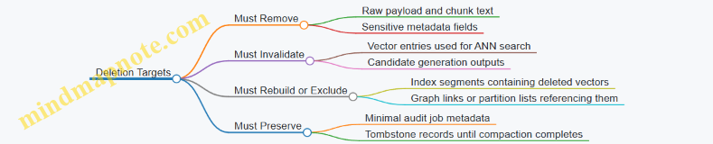
Checklist for Production Readiness
- Tombstones are enforced in every query path that can return candidates.
- Index maintenance removes deleted vectors from new segments.
- Verification confirms exclusion behavior, not just successful job completion.
- Audit logs contain only non-sensitive identifiers and status.
- Deletion jobs are idempotent and retry-safe.
When these pieces line up, deletion becomes a controlled workflow rather than a hope-and-pray operation.
12. Reference Implementations and End to End Engineering Examples
12.1 Building a Minimal Vector Search Service With Sharding
A minimal vector search service has three jobs: accept a query, find the nearest vectors, and return ranked results with enough metadata to be useful. Sharding adds one more job: route work to the right subset of data and merge partial rankings into a single top-k list.
Core Components
Start with a small, explicit contract between components.
- Ingestion path: store vectors plus an ID and optional metadata fields.
- Query path: embed the query text, run nearest-neighbor search on shards, merge results.
- Index path: build an index per shard so search is faster than brute force.
A practical minimal choice is to keep the index in memory per shard and persist raw vectors to disk. That keeps the system understandable while still demonstrating the operational shape.
Data Model and Shard Key
Each vector record should include:
id: stable identifiervector: fixed-length float arraymetadata: small JSON-like payload (e.g.,doc_id,tenant_id,lang)
Choose a shard key that is easy to compute at ingestion time and at query time. A common minimal approach is hashing tenant_id into N shards. That makes routing deterministic and avoids cross-shard scans.
Example: if tenant_id = "acme" hashes to shard 3, then all vectors for that tenant live on shard 3. Queries for acme only fan out to shard 3.
Minimal Service API
Use two endpoints.
POST /ingest: accepts a batch of vectors for a tenantPOST /search: accepts a query embedding or raw text plus filters
Keep filters simple at first. If you support tenant_id, route by shard key and only apply additional metadata filtering after candidate retrieval.
Shard Layout and Routing
Each shard runs the same local logic:
- store vectors and IDs
- maintain a local ANN or exact index
- answer
search(vector, k)returning(id, score)pairs
The router service does:
- compute shard(s) from
tenant_id - send the query to each selected shard
- merge results and return top-k
Mind the merge: if each shard returns top-k, the global top-k is not guaranteed to be the union of shard top-k unless you request enough candidates. A minimal safe rule is to request k * fanout per shard and then trim to k.
Mind Map: Minimal Sharded Vector Search
Example: End-to-End Request and Response
Ingestion request (conceptual):
- tenant:
acme - vectors: 10 records with IDs
v1..v10
Routing outcome:
- shard =
hash("acme") % N
Search request:
- tenant:
acme - query: embedding
q - k: 5
Shard response:
- shard returns 5 candidates
(id, score)sorted locally
Router merge:
- since fanout is 1, global top-5 is the shard top-5
If you later allow queries without tenant_id, you can fan out to all shards. Then request k * N candidates total, merge, and trim to k.
Minimal Implementation Sketch
Below is a compact outline showing the router and shard interfaces. It omits the embedding model and focuses on the sharding mechanics.
class Shard:
    def __init__(self, shard_id):
        self.shard_id = shard_id
        self.vectors = {}  # id -> vector
        self.index = None  # build after ingest

    def build_index(self):
        # Create Local Index over Self.vectors
        self.index = "local_index"

    def search(self, query_vec, k):
        # Return List of (id, Score) Sorted by Best Score
        return [("id1", 0.91), ("id2", 0.88)][:k]

class Router:
    def __init__(self, shards):
        self.shards = shards
        self.N = len(shards)

    def shard_for_tenant(self, tenant_id):
        return hash(tenant_id) % self.N

    def search(self, tenant_id, query_vec, k):
        sid = self.shard_for_tenant(tenant_id)
        candidates = self.shards[sid].search(query_vec, k)
        candidates.sort(key=lambda x: (-x[1], x[0]))
        return candidates[:k]
Operational Details That Prevent Surprises
- Index rebuild timing: build the shard index after ingest batches, not after every single vector, to keep latency predictable.
- Stable ordering: when scores tie, sort by
idso repeated queries return the same order. - Score meaning: decide whether higher is better (cosine similarity) or lower is better (distance) and keep it consistent across shards.
- Validation: during development, compare shard search results against brute force on a small dataset to catch indexing mistakes.
A minimal sharded service is small enough to reason about, yet structured enough to scale: ingestion writes to one shard, search routes deterministically, and merging produces a single ranked answer.
12.2 Implementing Approximate Search with Quantization and Reranking
Approximate search is what you use when exact k nearest neighbors is too slow or too memory-hungry. The usual pattern is: generate a small candidate set quickly using an approximate index, then compute more accurate scores for those candidates using reranking. Quantization helps the first stage by shrinking vector storage and speeding distance computations.
Mind Map: Approximate Search with Quantization and Reranking
Quantization Foundations That Matter in Practice
Quantization maps each high-dimensional vector to a compact code. Instead of storing full float32 vectors, you store codes plus the information needed to approximate distances.
A common approach is product quantization. Split a vector into M sub-vectors. For each sub-vector position m, learn a codebook of K centroids. Each original sub-vector is replaced by the index of its nearest centroid. Storage becomes M bytes or bits per vector depending on K, plus codebooks.
Distance estimation then becomes a lookup problem. For a query, you compute the distance from each query sub-vector to every centroid in each codebook. For a database vector, its approximate distance is the sum of the precomputed lookup values indexed by its stored code. This avoids scanning full vectors and reduces memory bandwidth.
Example: Product Quantization Candidate Generation
Suppose vectors are 768 dimensions and you choose M = 24 sub-vectors of 32 dimensions each. Choose K = 256 centroids per sub-vector. Each vector stores 24 code bytes.
At query time:
- Split the query into 24 sub-vectors.
- For each sub-vector position m, compute 256 distances to the m-th codebook centroids.
- For each candidate vector code, sum 24 lookup values to get an approximate distance.
- Keep the top N candidates (for example N = 200) for reranking.
This is fast because the inner loop is just table lookups and additions.
Building the Approximate Index with Quantization
You need two artifacts: the quantizer (codebooks) and the approximate structure that decides which candidates to consider.
A practical workflow:
- Train codebooks on a representative sample of embeddings.
- Encode all stored vectors into PQ codes.
- Build an approximate retrieval structure over the encoded data.
The approximate structure can be partition-based or graph-based. The key engineering point is that it should operate on the same distance notion you use for candidate selection. If your candidate generator uses approximate distances, your reranker must be able to correct them.
Reranking That Restores Accuracy
Reranking recomputes a more accurate score for the candidate set. The simplest version uses the original vectors and computes exact cosine similarity or inner product for the top N candidates.
If you store only quantized codes and not the original vectors, reranking becomes limited. Many systems keep original vectors for at least the top-level reranking stage, often in a separate memory tier.
A robust reranking procedure:
- Apply the same metadata filters used in candidate generation.
- Compute exact similarity for each candidate.
- Sort by score descending.
- Use deterministic tie-breaking, such as document id ascending.
Determinism matters because small score ties can otherwise cause pagination instability.
Example: Filter-Aware Candidate Generation and Reranking
Imagine each vector belongs to a tenant and a document type. You want top-k results for tenant T and type X.
- Candidate generation: route the query to shards that contain tenant T, then use the quantized index to produce top N candidates that also satisfy type X.
- Reranking: for those candidates, compute exact similarity using original vectors, then output top-k.
If you apply the filter only after reranking, you risk wasting reranking compute on candidates that will be discarded. If you apply it only during candidate generation, you must ensure the approximate structure does not accidentally exclude valid candidates due to filter routing mistakes.
Mind Map: Implementation Checklist
Minimal Pseudocode for the Two-Stage Flow
function search(query, k, N, filters):
  candidates = approx_index.search(query, N, filters)
  scored = []
  for id in candidates:
    if not matches(filters, id):
      continue
    score = exact_similarity(query, original_vector[id])
    scored.append((id, score))
  sort scored by score desc, id asc
  return first k ids from scored
Practical Tuning Knobs That Avoid Surprises
Start with N large enough that reranking can recover from candidate-generation errors. If recall is low, increase N before changing quantization parameters. If memory is the constraint, reduce K or M carefully and re-evaluate recall.
Also measure where time goes. If reranking dominates latency, you can reduce N, but only after confirming that recall@k stays within your target. If candidate generation dominates, you may need to adjust the approximate structure parameters or improve cache locality for lookup tables.
12.3 Designing an Index Build Pipeline With Validation And Compaction
A solid index build pipeline has two jobs: produce an index that matches the data you think you indexed, and keep it correct as new data arrives. The trick is to treat index construction like a reproducible build, not a one-off batch job.
Start with Inputs That Are Boringly Deterministic
Define the build contract up front: which embedding model version, which preprocessing steps, which vector normalization rule, and which metadata schema are used. Store these as build parameters alongside the output index. A practical pattern is to compute a content hash over the embedding inputs (document IDs plus raw text or image bytes) and over the model configuration. If the hash changes, you rebuild; if it doesn’t, you reuse.
Example: if you embed “doc 1042” with a new normalization setting, the vector values change even if the text is identical. Your pipeline should detect that via the build parameters hash, not via a human noticing a difference.
Stage the Build into Clear Phases
Use a multi-stage pipeline so failures are localized and reruns are cheap.
- Extract: pull the latest snapshot of records for a build window.
- Embed: generate vectors and attach metadata fields.
- Partition: assign records to shards or partitions using a stable rule (for example, consistent hashing on document ID).
- Index Build: construct the ANN structure per partition.
- Package: write index files plus a manifest describing parameters, counts, and checksums.
A good manifest includes: partition ID list, vector dimension, metric type, embedding model ID, normalization flag, and the number of vectors per partition.
Validate Early, Validate Often
Validation should catch problems before they become “why are results weird?” tickets.
3.1 Schema and Shape Checks
- Verify vector dimension matches the index configuration.
- Verify metric compatibility (cosine vs inner product) with the normalization rule.
- Verify metadata fields required for filters exist and have expected types.
3.2 Data Coverage Checks
- Compare record counts between the extracted snapshot and the embedded output.
- Ensure every record ID in the snapshot appears in exactly one partition.
3.3 Numerical Sanity Checks
- Reject vectors containing NaNs or infinities.
- Optionally compute simple stats per partition (min/max norms, percent of near-zero vectors). If a partition suddenly has many near-zero norms, you likely embedded the wrong content or applied the wrong preprocessing.
3.4 Index Correctness Checks Run a small offline verification set: for a sampled set of queries, compare approximate results against an exact baseline for recall@k. Also verify that the index returns only vectors that match filter constraints when filters are enabled.
Example: if your filter is “category = electronics,” a correctness check should confirm that every returned candidate belongs to that category. If not, you have a filter pushdown or metadata mapping bug.
Use a Two-Track Output Strategy
To keep production stable, separate “build artifacts” from “active index.”
- Build artifacts: immutable index files written to a staging location.
- Active index: a pointer (manifest reference) that production queries use.
Promotion happens only after validation passes. If validation fails, you keep the previous active index and investigate without interrupting queries.
Compaction Keeps the Index Clean
Compaction merges multiple index segments created over time (for example, base segments plus incremental segments). Without compaction, you accumulate many small segments, which increases query fanout and complicates deletion handling.
5.1 Segment Model Represent each segment with:
- a time range or ingestion range,
- a deletion bitmap or tombstone list,
- its own manifest and checksums.
5.2 Merge Policy Pick a merge policy based on segment sizes and query load. A common approach is to compact when the number of segments exceeds a threshold or when small segments dominate.
5.3 Compaction Validation After merging, re-run:
- vector count checks per partition,
- filter correctness checks on the same verification query set,
- recall@k checks on a small sample.
Example: if deletions are represented as tombstones, compaction must ensure those vectors are excluded from the merged index. A simple check is to pick a handful of deleted IDs and confirm they never appear in top-k for queries that would otherwise retrieve them.
Mind Map of the Pipeline
Mind Map: Index Build Pipeline with Validation and Compaction
Minimal Example Flow
- Extract records for build window
2026-02-15to2026-02-28. - Embed with model
m-embed-3and normalizationl2. - Partition by
hash(doc_id) mod N. - Build ANN per partition and write manifests with checksums.
- Validate shape, coverage, numerical sanity, and run recall@k on a fixed query set.
- If validation passes, promote the active index pointer to the new manifest.
- Periodically compact segments by merge policy, then validate deletion exclusion and filter correctness.
This structure keeps the pipeline predictable: you can rerun a failed phase, you can prove what you built, and you can merge segments without silently changing retrieval behavior.
12.4 Running Offline Evaluation with Ground Truth and Metrics
Offline evaluation answers a simple engineering question: “If we had the full dataset and perfect compute, what would the system return, and how close is our index to that ideal?” You start by defining ground truth, then measure retrieval quality and operational cost under the same constraints you expect in production.
Ground Truth Construction
Ground truth is a ranked list per query computed using an exact method. For vector search, the exact baseline is typically brute-force k-nearest neighbors using the same embedding model and the same similarity metric as the system under test.
A practical workflow:
- Freeze the embedding model and preprocessing so query and document vectors are comparable across runs.
- Select a representative query set (for example, 1k–50k queries) that matches your production distribution of intents and filters.
- Compute exact top-k per query on the evaluation corpus.
- Store results as
(query_id, doc_id, exact_rank, exact_score)so later metric computation is deterministic.
Example: Suppose you have 10,000 product descriptions and 2,000 search queries. For each query, you compute exact top-100 by cosine similarity. If your system uses metadata filters, you compute ground truth separately per filter combination or apply the filter during exact ranking.
Metric Selection That Matches Your Use Case
Different metrics reward different behaviors. Choose metrics that reflect what “good” means for your application.
Ranking quality metrics
- Recall@k: fraction of relevant items found in top-k. It’s intuitive for candidate generation.
- Precision@k: fraction of returned items that are relevant. It’s useful when users see only a few results.
- MRR: rewards placing the first relevant item early. It’s helpful when there’s usually one best answer.
- NDCG@k: handles graded relevance, such as “exact match” vs “related match.”
Ranking stability metrics
- Kendall tau or Spearman correlation between runs: useful when you compare index versions and want to avoid surprising reorderings.
Efficiency metrics
- Latency percentiles for offline queries (p50/p95/p99).
- Queries per second at fixed batch size.
- Memory footprint of the index and auxiliary structures.
A good rule: report at least one quality metric and one efficiency metric for each index configuration.
Relevance Labels and Their Sources
Offline metrics require relevance. In vector search, relevance can come from:
- Human judgments for a small set of queries.
- Click or interaction logs mapped to query-document pairs.
- Heuristic labels such as exact keyword matches that are known to correlate with relevance.
When labels are noisy, metrics still help you compare configurations, but you should interpret absolute values cautiously. For example, if “relevant” is derived from clicks, a document might be truly good but never clicked, which depresses recall.
Evaluation Harness Design
Your harness should make comparisons fair.
- Use the same query preprocessing as production, including normalization.
- Apply the same filter logic and verify that the candidate set respects it.
- Control randomness by fixing seeds and disabling nondeterministic tie-breaking.
- Run multiple trials if the index uses stochastic components.
Example harness logic:
- For each query, request top-k from the system.
- Compare returned doc_ids to the ground truth relevant set.
- Compute metrics and aggregate by query segments (for example, by document length bucket or filter selectivity).
Segment Analysis That Prevents “Average Wins”
A single overall number can hide failures. Segment your evaluation by factors that affect retrieval.
- Filter selectivity: how many documents match the metadata filter.
- Vector density: queries whose nearest neighbors are tightly clustered versus spread out.
- Embedding norms if you do not normalize.
Example: An index configuration might show Recall@10 = 0.62 overall, but Recall@10 = 0.30 for highly selective filters. That tells you the routing or filter pushdown path is the bottleneck.
Mind Map: Offline Evaluation Pipeline
Example: Metric Computation with Recall@k
If ground truth defines a relevant set R(q) for query q, then:
Recall@k(q) = |returned(q, k) ∩ R(q)| / |R(q)|
Example: If R(q) has 5 relevant documents and your system returns 3 of them in top-10, then Recall@10(q) = 3/5 = 0.6. Averaging over queries gives the overall Recall@10.
Example: Reporting a Configuration Comparison
Report a small table per index configuration with both quality and efficiency. Include the same query set and the same ground truth.
| Config | Recall@10 | NDCG@10 | MRR | p95 Latency (ms) | Index Memory |
|---|---|---|---|---|---|
| Exact baseline | 1.00 | 1.00 | 0.82 | 120 | N/A |
| ANN A | 0.72 | 0.66 | 0.61 | 18 | 40 GB |
| ANN B | 0.69 | 0.64 | 0.59 | 12 | 28 GB |
The point is not to crown a winner blindly; it’s to choose the configuration that meets your quality target while staying within your latency and memory budgets.
Common Pitfalls to Avoid
- Metric mismatch: using Recall@k when your application cares about first-result quality.
- Filter leakage: computing ground truth without applying filters, then comparing to a filtered system.
- Embedding drift: evaluating with vectors produced by a different model version than production.
- Unfair batching: comparing configurations with different batch sizes or concurrency.
Mind Map: What to Validate Before Trusting Results
A solid offline evaluation produces numbers you can defend: ground truth is computed exactly under the same assumptions, metrics match the user experience, and segment analysis explains why a configuration works or fails.
12.5 Operating a Production Retrieval Stack with Monitoring and SLOs
A production retrieval stack has three jobs: serve queries fast, return results that are consistently correct for the chosen definition of “similar,” and fail in ways that are predictable. Monitoring and SLOs tie those jobs to measurable signals, so you can fix the right thing instead of chasing symptoms.
Mind Map: Monitoring and SLOs
Defining SLOs That Match User Experience
Start with three SLO categories: latency, quality, and availability. Latency SLOs should be per user-facing endpoint, not just internal components. If you measure only average latency, you will miss the tail where fanout merges and reranking live.
Quality SLOs need a concrete metric. For example, if your app shows the top 10 items, define Recall@10 on a sampled set of queries with ground truth built from an exact search baseline. Also track filter correctness: the fraction of responses where every returned item satisfies the metadata predicate. This catches “almost right” failures where the index returns good neighbors but the filter logic is wrong.
Availability SLOs should reflect partial failures. If one shard fails and you still return results from others, decide whether that counts as success. Many teams treat “any results returned” as success, but that can hide systemic shard issues. A better approach is to define success as “results returned with expected coverage,” such as at least N shards contacted or a minimum candidate count.
Instrumentation That Separates Stages
Instrument the pipeline so each metric maps to a stage. A typical flow is: embed query → route to shards → retrieve candidates → apply filters → rerank → merge top-k.
For tracing, propagate a request id and record timestamps for each stage. For metrics, track candidate counts per shard and after filtering. If candidate counts suddenly drop, you can infer that the index or filter pushdown is misbehaving without waiting for quality metrics to lag.
Example: suppose P95 latency rises from 120 ms to 220 ms. If tracing shows shard retrieval time stable but reranking time doubled, you likely changed reranker batch sizing or increased candidate volume. If both retrieval and reranking rise, you may be under-provisioned or experiencing backpressure.
Monitoring Signals That Catch Real Failures
Use a small set of high-signal metrics:
- Fanout success rate: how often all intended shards respond.
- Queue depth and rejection counts: whether the service is overloaded.
- Candidate count distribution: mean and percentiles before and after filtering.
- Score distribution sanity: track min/max and percentile spread of similarity scores. A sudden collapse can indicate embedding normalization changes or a model version mismatch.
- Index version coverage: ensure the request hits the intended index build.
Quality monitoring should be sampled and replayed. For instance, take 1% of production queries every hour, store the query embedding id and filter predicate, and run an offline evaluation job that computes Recall@10 and filter correctness. This avoids expensive online ground truth while still detecting regressions quickly.
Alerting and Runbooks That Reduce Time to Fix
Alerts should be actionable. A latency alert should include which stage is responsible, based on recent trace aggregates. An error-rate alert should include whether failures are concentrated in specific shards or specific index versions.
Example runbook trigger:
- Condition: P95 latency exceeds SLO for 10 minutes AND reranker time exceeds its baseline by 50%.
- Immediate mitigation: reduce rerank depth from 200 candidates to 100, keeping the same top-k output size.
- Verification: confirm candidate counts remain stable and Recall@10 on the next sampled batch does not drop below an agreed threshold.
Example: A Minimal SLO Dashboard Layout
Use one dashboard per endpoint with three panels:
- Latency panel: P50/P95/P99 over time, plus stage breakdown for the last 30 minutes.
- Quality panel: Recall@10 and filter correctness from hourly sampled evaluation.
- Reliability panel: success rate, fanout success rate, and error budget burn.
Keep the dashboard readable by limiting it to metrics that map directly to the SLOs. If a metric cannot explain an SLO change, it probably belongs in a deeper diagnostic view.
Example: Incident Triage Without Guesswork
When an incident starts, triage in this order:
- Check fanout success rate. If it drops, focus on shard health and routing.
- Check candidate counts. If they drop, focus on index retrieval parameters or filter pushdown.
- Check reranker time. If it spikes, focus on batching, model version, or input size.
- Check score distribution sanity. If it shifts, focus on embedding normalization and model version alignment.
This sequence narrows the search space quickly because each step corresponds to a distinct failure mode.
Operational Discipline That Keeps SLOs Stable
SLOs are not just monitored; they are maintained. Enforce index versioning so you can correlate quality changes with specific builds. Validate schema changes that affect filters, because a small mismatch can silently reduce filter correctness while leaving latency unchanged. Finally, treat evaluation jobs as part of the system: if ground truth sampling stops, quality SLOs become guesses, not measurements.