Mastering QUIC and HTTP3 Protocols
1. Foundations of QUIC and HTTP3
1.1 Transport Layer Goals and Constraints for Modern Web Traffic
Modern web traffic has two jobs at once: move bytes reliably enough to make applications correct, and move them quickly enough to make users feel in control. The transport layer is where those goals meet real network constraints—loss, delay, reordering, limited bandwidth, and changing paths.
Transport Layer Goals
Correctness Under Imperfect Networks
A transport protocol must define what it means for data to be “delivered.” For many web uses, correctness includes ordered delivery for some byte sequences, reliable delivery for others, and clear error signaling when delivery cannot be completed. If the application can’t tell whether a request body arrived intact, it can’t safely retry or render partial results.
A practical example: a browser downloading a JSON response. If a few bytes flip due to corruption, the JSON parser will fail. The transport layer should either prevent corruption from reaching the application (via integrity checks) or detect failure early enough that the application can retry.
Performance That Matches Application Behavior
Different applications tolerate different tradeoffs. Interactive actions (typing, scrolling, pointer movement) prefer low latency even if some data is dropped. File transfers prefer throughput and completeness. A transport layer goal is to provide mechanisms that let applications choose how to balance these needs.
Example: a chat app sending small messages. Waiting for strict in-order delivery of every earlier message can delay the latest one. A transport design that supports multiple independent data paths (streams) lets the app prioritize what matters now.
Efficient Use of Network Resources
Transport protocols influence congestion and fairness. If a protocol injects too much traffic, it can worsen loss for everyone. If it backs off too aggressively, it wastes available capacity. The transport layer must react to congestion signals without requiring perfect knowledge of the network.
Example: when a mobile client switches from Wi‑Fi to LTE, available capacity changes. A well-behaved transport adapts its sending rate based on observed delivery behavior rather than assuming the old network still applies.
Transport Layer Constraints
Loss, Reordering, and Delay
Loss is common: wireless links drop packets, routers buffer and overflow, and middleboxes may interfere. Reordering happens when packets take different routes or when queues drain at different rates. Delay varies with queueing and scheduling.
Example: a video stream where packet 20 arrives before packet 19. If the transport insists on strict ordering for the entire stream, the application may stall waiting for missing earlier data, even though later frames are already available.
Limited MTU and Fragmentation Risk
Packets have a maximum size. If a protocol sends larger datagrams than the path supports, fragmentation may occur or be dropped. Either outcome reduces effective throughput and can increase loss.
Example: a client sending a large header block. If the transport can avoid oversized packets, it reduces the chance that the network discards the entire packet.
Middleboxes and Path Changes
Many networks rewrite addresses, translate ports, or change routes. Some devices also impose timeouts that silently remove state.
Example: a NAT mapping that expires during a quiet period. When traffic resumes, the server may see packets from a different apparent path. Transport protocols need a defined strategy for continuing communication or failing cleanly.
Mind Map: Transport Layer Goals and Constraints
Putting It Together with a Worked Scenario
Consider a browser loading a page with both a small HTML response and a larger media asset. The transport layer should:
- Deliver the HTML quickly and reliably enough for rendering. If a few packets are lost, recovery should be fast for small objects.
- Continue transferring the media without letting missing earlier bytes block newer frames. Stream independence helps here.
- Avoid flooding the network. Congestion control should slow down when loss rises, but it should not treat every loss as a reason to stop entirely.
- Handle path changes. If the client’s network changes mid-transfer, the protocol should either migrate cleanly or fail in a way that the application can retry.
In short, the transport layer is a contract: it defines how data moves, how failures are detected, and how the protocol behaves when the network misbehaves. QUIC and HTTP/3 build on that contract with specific mechanisms that target these exact goals and constraints.
1.2 QUIC Design Overview and How It Differs from TCP and TLS
QUIC is a transport protocol that combines reliability, multiplexing, and cryptographic protection into one layer that runs over UDP. That single design choice changes the shape of the problem: instead of relying on TCP for ordered delivery and TLS for encryption, QUIC builds those behaviors into its own packet processing and state machines.
What QUIC Changes Compared to TCP
TCP offers a byte stream with in-order delivery, plus congestion control and retransmission. QUIC instead offers multiple independent streams over a single connection, where each stream can make progress even when others stall. This matters because TCP’s in-order rule couples unrelated data: if one segment is lost, the receiver may have to wait before delivering later bytes to the application.
QUIC still detects loss and retransmits, but it does so using packet numbers and acknowledgments at the QUIC layer. That means QUIC can track loss per packet and recover without forcing the application to wait for a single global byte stream.
QUIC also treats connection identity as a first-class concept. TCP connections are tied to the 4-tuple of IP addresses and ports, so address changes typically break the connection. QUIC uses connection identifiers so the connection can survive path changes while keeping the cryptographic context intact.
What QUIC Changes Compared to TLS
TLS 1.3 defines handshake messages and key derivation, but it assumes a reliable transport underneath. QUIC integrates TLS 1.3 semantics while adapting them to UDP’s realities: packets can be reordered, duplicated, or lost without the transport layer guaranteeing delivery.
In QUIC, the handshake and encryption keys are established as part of the connection state. After keys are available, QUIC encrypts application data and most handshake traffic, so middleboxes see only encrypted payloads and metadata defined by the protocol. This reduces the number of moving parts that must coordinate across layers.
QUIC also supports 0-RTT data, which allows sending application bytes early using keys derived from a prior handshake. The protocol includes replay-safety rules so early data is not blindly accepted in situations where it could be replayed.
Core QUIC Building Blocks
A QUIC connection is a set of cryptographic keys plus transport state. That state includes:
- Packet number spaces for different phases of the connection.
- Loss detection rules and acknowledgment generation.
- Congestion control state that governs how many bytes may be in flight.
- Stream state for each logical stream.
Each QUIC packet carries one or more frames. Frames are small units of meaning, such as stream data, acknowledgments, or control information. This frame-based approach lets QUIC interleave control and data efficiently.
Example: Why Independent Streams Matter
Imagine a web page that loads a large image and a small JSON response. With TCP, if a lost segment occurs in the image flow, the receiver may delay delivering later bytes to the application because the byte stream must remain ordered. With QUIC, the JSON can be carried on a different stream. If the JSON stream’s packets arrive, the application can process them immediately, while the image stream waits for retransmission.
Example: Acknowledgments and Loss Detection in Practice
Consider a receiver that gets packet numbers 10, 12, and 13, but not 11. QUIC can acknowledge receipt of 10 and 12–13 and mark 11 as missing. When the sender receives those acknowledgments, it can retransmit packet 11 without waiting for a later packet to arrive in order. The application sees fewer stalls because the transport layer recovers at the packet level rather than at the byte-stream level.
Example: Handshake State and Encryption Timing
A typical flow is:
- Client sends initial packets that include handshake messages.
- Server responds with handshake messages and establishes keys.
- Once application keys are active, QUIC encrypts application frames.
If 0-RTT is used, the client may send application frames earlier, but the server applies replay-safety checks before treating that data as fully committed.
Summary of the Differences
QUIC differs from TCP by moving reliability, loss recovery, and congestion control into the protocol itself while offering multiplexed streams that avoid global in-order coupling. It differs from TLS by integrating the TLS 1.3 handshake and keying into QUIC’s packet and state machinery so encryption and transport behavior are coordinated rather than layered. The result is a single transport protocol that can handle UDP’s quirks without forcing the application to pay the price.
1.3 HTTP3 Mapping to QUIC Streams and Frames
HTTP/3 rides on QUIC, but it does not replace QUIC’s job. QUIC still handles packetization, encryption, loss recovery, and congestion control. HTTP/3’s job is to define how HTTP messages are represented as QUIC streams and how HTTP semantics are carried in QUIC frames.
Core Mapping Model
Think of QUIC as the transport “plumbing” and HTTP/3 as the “message layout.” QUIC provides:
- Connections identified by connection IDs.
- Streams that carry ordered byte sequences.
- Frames that carry control information and stream data.
HTTP/3 then assigns meaning to those pieces:
- Each request/response pair uses one or more QUIC streams for the body and uses a separate mechanism for headers.
- Headers are compressed with QPACK, which introduces additional coordination streams.
- HTTP errors are expressed using stream-level resets and HTTP-specific error codes, not by inventing new transport behavior.
Stream Roles in HTTP/3
HTTP/3 uses three practical stream categories.
Request and Response Streams
- A request typically maps to a bidirectional stream where the client sends request headers and then request body bytes.
- A response maps to a bidirectional or unidirectional stream depending on implementation choices, but the common pattern is that the server sends response headers and then response body bytes on a stream dedicated to that response.
Because QUIC streams are ordered, HTTP/3 can treat the byte stream as the ordered sequence of HTTP message components for that specific request.
Control Streams for QPACK
QPACK needs coordination so the decoder can use dynamic header table entries without stalling. That coordination uses dedicated streams:
- An encoder stream carries instructions from the encoder to the decoder.
- A decoder stream carries acknowledgments and requests that let the encoder know what the decoder can safely reference.
This is why HTTP/3 header compression can remain efficient even when packet loss happens: the transport can recover lost packets, while QPACK avoids blocking the entire connection.
Unidirectional vs Bidirectional Streams
QUIC supports both. HTTP/3 uses unidirectional streams for QPACK coordination because those directions are naturally one-way: encoder-to-decoder and decoder-to-encoder. Using unidirectional streams keeps the mental model clean: you know which side is responsible for producing which bytes.
Frame Types and How HTTP3 Uses Them
At the QUIC layer, frames include stream data and transport control. HTTP/3 relies on QUIC’s frames rather than defining a new packet format.
- Stream Data Frames carry the actual bytes of HTTP/3 message components.
- Control Frames manage QUIC-level behavior like acknowledgments and flow control.
HTTP/3 defines how to interpret the bytes inside stream data. For example, the beginning of a request stream contains header-related information encoded for HTTP/3, and later bytes contain body data.
Worked Example: One Request Through the Mapping
Suppose a client sends a GET request.
- QUIC establishes an encrypted connection.
- The client opens a stream for the request.
- The client sends request headers on that stream using HTTP/3’s header representation.
- The server opens or uses a response stream and sends response headers.
- The server streams response body bytes on the response stream.
- In parallel, QPACK coordination streams exchange dynamic table updates and acknowledgments.
Here’s a compact view of the stream interactions.
    flowchart LR
  C[Client] -->|QUIC connection| S[Server]
  C -->|Request stream| RS[Request Stream]
  S -->|Response stream| RSP[Response Stream]
  C -->|QPACK encoder instructions| E[QPACK Encoder Stream]
  S -->|QPACK decoder acknowledgments| D[QPACK Decoder Stream]
  RS -->|HTTP/3 headers and body bytes| S
  RSP -->|HTTP/3 headers and body bytes| C
Mind Map: HTTP3 Over QUIC
Practical Implication for Implementers
When you implement HTTP/3, you should treat “stream boundaries” as message boundaries. A common bug is to assume that headers and body bytes can be arbitrarily interleaved across streams. In HTTP/3, the mapping is designed so that each stream carries a coherent ordered sequence for its role, while QPACK coordination happens on separate streams.
That separation is the whole point: QUIC can recover lost packets without confusing HTTP message structure, and HTTP/3 can compress headers without stalling every request.
1.4 Packetization, Connection Identifiers, and Multiplexing Basics with Worked Examples
QUIC packetization is the practical bridge between “protocol rules” and “what actually moves across the network.” It also explains why QUIC can keep multiple conversations alive even when addresses change, and why one slow stream doesn’t automatically stall everything else.
Packetization Basics
A QUIC packet is a datagram that carries one or more frames. Frames are the units of work: stream data, acknowledgments, flow-control updates, and so on. Packetization matters because it determines how quickly the receiver can act on useful information.
Key idea: QUIC tries to send frames in packets that fit the path’s effective MTU. If you send too large packets, fragmentation or loss increases, and loss recovery has to do more work.
Worked Example: Choosing a Packet Size for Stream Data
Suppose your path MTU is 1200 bytes (common for safe UDP payload sizing). You reserve space for QUIC and UDP headers, leaving room for stream data. If you send 1,200 bytes of stream data per packet, you risk overshooting after header overhead. Instead, you pick a payload budget that stays under the safe limit.
A simple rule of thumb for reasoning: if your implementation can estimate header overhead, set the stream chunk size so that UDP payload <= MTU - headers. The receiver then gets complete frames without relying on IP fragmentation.
Connection Identifiers
QUIC uses Connection IDs (CIDs) to identify a connection even when the 5-tuple (source IP, source port, destination IP, destination port, protocol) changes. This is crucial for NAT rebinding, mobility, and route changes.
A CID is carried in packets so the receiver can map incoming packets to the right connection state. When the address changes, the CID stays the same, so the receiver can continue without treating the new path as a brand-new connection.
Worked Example: NAT Rebinding Without Losing the Connection
Imagine a client behind a NAT. The client’s Wi‑Fi changes networks, and the NAT assigns a new external port. If the protocol relied only on the 5-tuple, the server would see packets from a different address and likely discard them as unknown. With CIDs, the server reads the CID from the packet header, finds the existing connection context, and continues.
The practical consequence: you can design your application to tolerate address changes without re-establishing everything. QUIC still needs to validate that the new path is legitimate, but the CID prevents the “identity reset” that TCP would suffer.
Multiplexing Basics
Multiplexing means multiple independent streams share the same QUIC connection. QUIC avoids head-of-line blocking at the transport level by allowing frames from different streams to interleave in packets.
However, multiplexing is not magic. Flow control and scheduling still decide which stream’s data gets sent first, and receiver-side buffering can still create delays if one stream floods.
Worked Example: Two Streams, One Interactive and One Bulk
Consider:
- Stream A: chat messages, small and latency-sensitive.
- Stream B: file upload, large and bandwidth-hungry.
If you always send Stream B frames whenever you have space, Stream A frames may wait behind bulk data, increasing perceived latency. A better approach is to schedule Stream A frames with higher priority.
A simple scheduling strategy for reasoning:
- Maintain per-stream queues.
- Each packet budget is filled by selecting frames from the highest-priority non-empty stream.
- After sending a small burst from Stream A, allow some progress for Stream B.
This keeps interactive messages from being stuck behind large transfers, while still using available bandwidth.
Mind Map: How Packetization, Connection IDs, and Multiplexing Fit Together
Worked Example: Putting It All Together in a Packet Timeline
Assume the client has one QUIC connection with a stable CID. It sends two streams.
- Client sends packet P1 containing Stream A frames (a short message) and a small acknowledgment frame.
- Client sends packet P2 containing Stream B frames (bulk data).
- Midway, the client’s network path changes and the NAT assigns a new port. The client continues sending packets P3 and P4 with the same CID.
- Server receives P3, reads the CID, maps it to the existing connection, and continues processing.
- Stream A frames keep getting scheduled into early packet slots, so interactive latency stays low even while Stream B is still transferring.
The important detail is that each mechanism solves a different problem: packetization reduces avoidable loss and buffering, CIDs preserve connection identity across address changes, and multiplexing plus scheduling prevents one stream’s behavior from dominating the whole connection.
1.5 Practical Lab Setup for Capturing Traces and Verifying Behavior
A good lab setup answers two questions: what happened on the wire, and whether your implementation behaved according to the protocol rules you expect. The trick is to make the capture deterministic enough that you can compare runs, then to verify behavior at multiple layers: transport timing, stream semantics, and HTTP/3 frame ordering.
Lab Goals and What to Verify
Start by choosing a small set of behaviors to validate in each run.
- Handshake and keys: confirm the QUIC handshake completes and that application data appears only after keys are established.
- Loss and recovery: force loss and verify retransmission and ACK-driven recovery.
- Stream behavior: confirm stream creation, ordering expectations, and reset handling.
- HTTP/3 framing: verify that request/response semantics map to the expected QUIC streams and that header compression does not stall progress.
Mind Map: Trace Capture Workflow
Minimal Environment Setup
Use one machine for the client and one for the server to reduce noise. If you must run both on one host, still separate processes and keep CPU load stable.
- Pick a QUIC-capable HTTP/3 client and server that can emit logs and supports key logging for packet decryption.
- Enable key logging so packet captures can be decrypted into meaningful QUIC and HTTP/3 events.
- Use a fixed test script that sends a known sequence of requests and reads responses in a predictable order.
For timestamps, align three clocks: client logs, server logs, and capture time. If you cannot align perfectly, record relative offsets by marking a single event visible in both logs and captures, such as the first request send.
Network Emulation for Controlled Behavior
To verify loss recovery, you need repeatable impairment. Use a network emulator that can apply delay, jitter, and packet loss to a specific path.
Example: introduce a small delay and a modest loss rate so retransmissions occur without turning the test into a timeout festival.
# Example Network Emulation Profile
# Apply to the interface used by the client->server path
# Adjust Values to Match Your Environment
sudo tc qdisc add dev eth0 root netem delay 80ms 10ms loss 2%

# Run the Lab Test Script
# Then remove the rule
sudo tc qdisc del dev eth0 root
After each run, confirm the impairment actually applied by checking capture statistics for retransmissions and gaps in packet numbers.
Capturing Packets and Decrypting QUIC
Capture packets on the client side first. Client-side captures make it easier to correlate request send times with QUIC packet numbers.
- Packet capture: record UDP traffic for the server address and port.
- Key log: store key material in a file the capture tool can use.
- Decryption: use a decoder that understands QUIC and HTTP/3 so you can inspect frames and stream events.
# Packet Capture Command Example
# Capture only the QUIC/HTTP3 UDP flow
sudo tcpdump -i eth0 -s 0 -w quic_lab.pcap \
  udp and host SERVER_IP and port 4433

# Ensure Key Log Is Enabled in Your Client/server Process
# so the decoder can decrypt captured packets.
Verification Checklist with Concrete Evidence
Use a baseline run (no loss) and a perturbed run (with loss). Then verify the following in the decrypted view.
- Handshake timeline: confirm that the first application stream data appears after handshake completion.
- Packet number progression: ensure packet numbers advance monotonically and that retransmitted packets reuse the correct packet number space.
- ACK-driven recovery: verify that loss triggers retransmission and that later ACKs account for recovered data.
- Stream lifecycle: confirm stream creation occurs before data frames, and that stream resets terminate the stream cleanly.
- HTTP/3 frame ordering: check that request headers arrive before response headers on their respective streams, and that end-of-stream markers match the expected completion.
Mind Map: What to Look for in Decrypted Traces
Example Run Plan with Expected Outcomes
Run a single request that returns a small response, then repeat with a larger response that forces multiple QUIC packets.
- Baseline: you should see a clean handshake, then a short sequence of packets carrying request and response frames with minimal retransmission.
- Impairment: you should see at least one retransmission, followed by ACKs that confirm the receiver accepted the recovered data.
If you do not see retransmissions under loss, reduce loss rate only after confirming packet loss is present in the capture; otherwise you may be testing a path that bypasses the emulator.
Common Failure Modes and How to Spot Them
- No decryption: key logging missing or file path mismatch; you will only see encrypted payloads.
- Stream mismatch: HTTP/3 frames appear on unexpected streams; verify stream IDs and concurrency assumptions.
- QPACK stalls: response progress pauses until header decoding resources arrive; confirm insert/ack behavior in the trace.
- Timing confusion: logs and capture timestamps drift; re-run with a single marked event to compute offsets.
A lab run that produces a readable decrypted timeline is the win condition. Once you can point to specific packets, frames, and stream events, optimization becomes a matter of changing one variable at a time and re-checking the same evidence.
2. QUIC Connection Establishment and Security Handshake
2.1 QUIC Handshake Message Flow and State Transitions
A QUIC connection starts as a set of UDP packets that gradually become a cryptographically protected transport. The handshake is both a message exchange and a state machine: each side moves through well-defined states as it learns keys, validates the peer, and decides what data it is allowed to send.
Core Actors and What They Need
QUIC has two roles: the client initiates and the server responds. Both sides maintain:
- A connection ID pair so packets can be matched even if the network path changes.
- A cryptographic context that evolves from “no keys” to “handshake keys” to “1-RTT keys.”
- A packet protection level that determines which packets are allowed to carry which data.
The handshake is carried over QUIC packets, not separate TCP segments. That matters because QUIC can protect different packet number spaces differently, and it can decide when to accept or reject packets based on what keys are available.
Message Flow from First Packet to 1-RTT
-
Client Initial The client sends an Initial packet containing a TLS 1.3 ClientHello inside QUIC. At this point, the client uses Initial keys derived from a well-known mechanism so the server can authenticate the packet format and recover the handshake.
-
Server Initial and Handshake The server replies with an Initial packet that carries a TLS 1.3 ServerHello and related handshake messages. It also sends a Handshake packet when it has enough information to proceed. The server’s packets are protected with Handshake keys once those keys are established.
-
Client Handshake Completion The client sends its remaining handshake messages, typically including Finished. When the client receives the server’s Finished and verifies it, it can transition to using 1-RTT keys for application data.
-
Server Finalization The server verifies the client’s Finished. After that, both sides can treat the connection as established for 1-RTT protected traffic.
A key detail: QUIC can send application data only after the relevant keys are available and verified. Before that, packets are limited to handshake-related content.
State Transitions as a Practical Checklist
Think of the state machine as “what am I allowed to send and accept right now?” rather than “what label do I display.” Common transitions look like this:
- Before Keys: Only Initial packets are meaningful. Handshake packets are ignored because the receiver cannot decrypt them.
- Handshake Keys Available: Handshake packets become decryptable and verifiable. The receiver can process TLS handshake messages.
- 1-RTT Keys Available: Application streams may carry HTTP/3 frames (or other application data). Packets protected with 1-RTT keys are accepted.
- Validation Completed: The connection is considered established. Loss recovery and congestion control operate normally for the established packet protection level.
If a packet arrives “too early” (for example, a Handshake packet before the receiver can derive Handshake keys), the receiver discards it. This prevents confusing the state machine with data it cannot authenticate.
Mind Map: the Handshake Flow
Example: What Happens When a Packet Is Lost
Assume the client sends Initial packets numbered 1, 2, 3. Packet 2 is lost.
- The server can still process packet 1 and 3 if it can decrypt them and if the TLS handshake messages it needs are present.
- If the server’s ability to advance depends on a message that was only in packet 2, it will wait. It does not guess; it waits for retransmission.
- The client retransmits lost handshake-relevant data using the appropriate packet protection level.
This is why QUIC ties handshake progress to what is actually received and authenticated, not to what was sent.
Example: Early Data Boundaries Without Guessing
A client may attempt to send application data early, but it must still respect key availability and replay safety rules. If the server cannot validate the early data context, it can treat early application data as not authoritative and require the client to resend under 1-RTT keys.
The practical takeaway is simple: handshake state determines whether application bytes are “real” or “tentative,” and the receiver’s verification gates what it will act on.
Putting It Together with a Minimal Timeline
- Client Initial → Server Initial
- Server Handshake → Client Handshake
- Client Finished → Server verifies
- Server Finished → Client verifies
- Transition to 1-RTT → Application data allowed
The handshake is therefore a sequence of cryptographic readiness steps, each one backed by explicit state transitions that prevent the transport from accepting unauthenticated or premature information.
2.2 TLS 1.3 Integration and Key Derivation for QUIC
QUIC uses TLS 1.3 as its cryptographic engine, but it does not run TLS over a byte stream like TCP. Instead, QUIC carries TLS handshake messages inside QUIC packets, and it derives keys that are directly used to protect QUIC packets and to encrypt HTTP/3 traffic. The result is a clean separation: TLS defines the key schedule and authentication, while QUIC defines packet protection, loss recovery, and stream multiplexing.
Core Mapping Between TLS 1.3 and QUIC
TLS 1.3 has a handshake that produces traffic secrets for different phases. QUIC mirrors those phases with packet protection “epochs” so that packets sent at different times use different keys.
- Handshake messages travel in QUIC: QUIC transports the TLS handshake bytes, but QUIC still decides when to retransmit, how to number packets, and how to migrate paths.
- Traffic secrets become QUIC packet keys: TLS outputs secrets; QUIC turns them into AEAD keys and nonces used for packet encryption and integrity.
- Multiple encryption levels: QUIC typically uses separate keys for Initial, Handshake, and 1-RTT data, aligning with when the TLS handshake progresses.
Key Schedule Walkthrough with QUIC Phases
TLS 1.3’s key schedule starts from an input secret and expands it into a set of traffic secrets. QUIC then derives packet protection keys from those secrets.
-
ClientHello and server response
- The client sends a ClientHello.
- The server replies with ServerHello plus handshake messages.
- Both sides compute shared secrets from the negotiated key exchange.
-
Deriving handshake traffic secrets
- After ServerHello, TLS derives handshake traffic secrets.
- QUIC uses these to encrypt and authenticate packets carrying handshake data.
-
Deriving 1-RTT traffic secrets
- Once the handshake reaches the point where application data is allowed, TLS derives 1-RTT secrets.
- QUIC uses the 1-RTT secrets to protect application packets.
-
Finished messages as handshake integrity anchors
- TLS Finished messages prove that both sides computed the same handshake transcript.
- QUIC relies on these to ensure that the derived keys correspond to the authenticated handshake.
Packet Protection Key Derivation
QUIC uses AEAD, so each packet needs a key and a nonce construction. The key comes from the relevant traffic secret, and the nonce is built from a per-connection value plus the packet number.
A practical way to think about it:
- Key: stable for an encryption level (for example, 1-RTT).
- Nonce: changes per packet using the packet number, preventing reuse.
If you ever see repeated nonces under the same key, you have a serious bug. QUIC’s design makes nonce uniqueness a function of packet numbering and the encryption level.
Mind Map: TLS 1.3 Secrets to QUIC Packet Keys
Example: Tracing Which Keys Protect Which Packets
Imagine a client and server exchanging packets during connection setup.
- Packets containing ClientHello are protected using the QUIC Initial protection keys.
- Packets carrying handshake data after ServerHello use handshake protection keys.
- Packets carrying HTTP/3 frames use 1-RTT protection keys.
Even if the application starts sending early, QUIC must ensure that the packet protection keys match the handshake stage. That’s why QUIC separates encryption levels: it prevents the common mistake of using application keys before the handshake is authenticated.
Example: Why Transcript Matters
Suppose a middlebox drops a handshake packet. QUIC retransmits, but the transcript must remain consistent. TLS Finished messages bind the derived secrets to the exact handshake transcript. If retransmission logic accidentally changes what the transcript “looks like” to each side, the Finished verification fails, and the connection is terminated.
Practical Checklist for Implementers
- Ensure the TLS transcript used for Finished matches the handshake bytes as carried by QUIC.
- Derive AEAD keys from the correct TLS traffic secret for each QUIC encryption level.
- Construct nonces so that each (key, nonce) pair is unique per packet.
- Keep encryption-level transitions aligned with handshake state so application packets never use handshake keys.
Summary
TLS 1.3 provides the key schedule and handshake authentication; QUIC provides packetization, retransmission, and encryption-level separation. When these pieces align, QUIC gets strong confidentiality and integrity without sacrificing the transport behaviors that make it effective in real networks.
2.3 0-RTT Data Use With Replay Safety Requirements
0-RTT in QUIC lets a client send application data immediately after it starts a new connection, without waiting for the full handshake to complete. The trade is simple: early data is sent before the server has confirmed the client’s identity for this connection, so the protocol must prevent an attacker from replaying that early data to cause unintended effects.
Core Idea: Early Data Is Authenticated Later
In QUIC, the client uses keys derived from a previously established session to encrypt and authenticate 0-RTT packets. The server can decrypt them, but it still must decide whether to accept them for this new connection. Acceptance depends on replay safety rules and on whether the server can verify that the early data corresponds to a legitimate prior session.
A useful mental model is a two-step contract:
- The client encrypts early data so it cannot be read or modified in transit.
- The server applies replay controls so it can refuse early data that might be resent by an attacker.
Replay Safety Requirements: What Must Be True
Replay safety is about preventing “same request, repeated effect.” The protocol requirements can be summarized as follows.
First, the server must be able to detect or limit replays. If it cannot, it must not accept 0-RTT data that could change state.
Second, the server must provide a mechanism to the client so the client can learn whether early data was accepted. If the server rejects early data, the client must treat the corresponding application actions as not having happened.
Third, the server must ensure that any accepted 0-RTT data is bound to the correct cryptographic context. That binding is achieved through session resumption keys and the handshake transcript used in key derivation.
Practical Consequence: Idempotency Is Your Friend
Even with replay controls, the safest application design treats 0-RTT payloads as potentially duplicated. That means using idempotent operations for early requests, such as:
- “Get resource” requests that do not modify server state.
- “Create with client-generated id” patterns where duplicates map to the same outcome.
If you must perform non-idempotent actions, you need an application-level strategy that can detect duplicates, or you must avoid sending those actions as 0-RTT data.
Server-Side Replay Controls
Servers typically implement replay protection by requiring additional information tied to the resumption attempt. The server can then decide whether to accept early data for a given resumption token.
A concrete example: imagine a login flow where the client previously authenticated successfully. On a new connection, the client sends an early “resume session” request. If an attacker replays that early request from a different network path, the server should either:
- accept it only once per token, or
- accept it only when it can verify that the request is fresh for that client.
If the server cannot verify freshness, it should reject early data and force the client to retry after the handshake completes.
Client-Side Behavior: How to Handle Rejection
The client sends 0-RTT data optimistically, but it must be prepared for rejection. The client should:
- correlate early requests with a local “pending” state,
- wait for handshake completion signals,
- and only finalize application effects after confirmation.
A simple pattern is to buffer side effects until the server’s acceptance is known. For example, a client might render a page only after it knows the server accepted the early request that fetched it.
Mind Map: Replay Safety Requirements
Example: Idempotent Request with Client-Generated Token
Suppose an HTTP request triggers a server-side “mark notification as read.” If sent as 0-RTT, duplicates could cause incorrect counts or repeated audit entries.
A safer approach is:
- The client includes a unique request ID in the request payload.
- The server records processed request IDs per user.
- If the same request ID arrives again, the server returns the same result without repeating the side effect.
Even if an attacker replays the encrypted 0-RTT packet, the server’s idempotency check prevents repeated state changes.
Example: Buffering Side Effects Until Acceptance
Consider a client that sends an early “fetch profile” request and immediately updates local UI with the response. If the server rejects 0-RTT, the client must not treat the early response as authoritative.
A robust flow is:
- send early request,
- store the response data as “tentative,”
- finalize only after the handshake confirms acceptance.
This keeps the user experience consistent without relying on luck or timing.
Example: Server Rejects Early Data for Non-Idempotent Actions
If a server policy is strict, it can reject 0-RTT when the request indicates a state change. For instance, a request labeled “update settings” might be accepted only after the handshake completes.
The client then retries the same operation after confirmation. Because the operation is now post-handshake, the server can apply stronger guarantees and the client can safely commit the result.
2.4 Connection Migration and the Role of Connection Identifiers
Connection migration is what happens when a QUIC endpoint changes its network path while keeping the same logical connection. The tricky part is that IP addresses and UDP 5-tuples can change, but the application should not have to restart everything just because a Wi‑Fi link switched to cellular. QUIC handles this by separating “who you are” from “where you are right now,” and that separation is anchored by Connection IDs.
Why Migration Breaks Naive Transport Designs
If a transport identifies a connection only by the 5-tuple (source IP, source port, destination IP, destination port, protocol), then any path change looks like a brand-new connection. The peer would stop accepting packets from the new address, and the sender would keep retransmitting on the old path. QUIC avoids this by allowing the peer to recognize packets that belong to the same connection even when the network path changes.
Connection Identifiers as the Stable Handle
A Connection ID (CID) is carried in QUIC packets so that the receiver can map an incoming packet to the correct connection state. The CID is not meant to be secret; it is a routing key for the protocol. QUIC typically uses two CIDs per direction: one that the sender uses to identify itself to the peer, and one that the peer uses to identify back. This lets each side keep track of which CID it should expect on incoming packets.
A simple mental model: the CID is the “seat number,” while the IP/port tuple is the “current location of the theater.” If the theater moves, you still find the same seat.
Migration Mechanics Step by Step
Migration is not a single magic moment; it is a sequence of events that keeps both sides consistent.
- Path changes at the client: the client’s source address changes due to NAT rebinding, Wi‑Fi roaming, or switching networks.
- Client continues sending with the same connection identity: it sends packets on the new path, using the CID that the server expects for that client.
- Server receives packets from a new address: it uses the CID to locate the connection state and accepts the packet if it passes validation.
- Server validates reachability: the server must confirm that the client is reachable at the new path before it fully commits to it.
- Both sides converge on the new path: once validation succeeds, future packets flow on the new path without resetting the connection.
The reachability validation is important because accepting packets from a new address without checks could let an attacker inject traffic into an existing connection.
Address Validation and the Role of Stateless Tokens
QUIC uses an address validation mechanism based on tokens. The server issues a token tied to the client’s address context, and the client presents it when it wants the server to accept the new path. This keeps the server from blindly trusting the first packet that arrives from a new address.
Here is the flow in compact form.
    flowchart TD
  A[Client sends on old path] --> B[Server receives using CID]
  B --> C[Client changes network path]
  C --> D[Client sends on new path with expected CID]
  D --> E[Server maps CID to connection state]
  E --> F[Server requires address validation token]
  F --> G[Client includes token in new-path packets]
  G --> H[Server validates reachability]
  H --> I[Server updates active path]
  I --> J[Packets continue without connection reset]
Practical Example with Concrete Packet Behavior
Assume a client had been sending QUIC packets from 192.0.2.10:40000 to 203.0.113.5:443. After roaming, it now sends from 198.51.100.77:41012 to the same server.
- The client keeps using the CID that the server associated with this connection.
- The server receives a packet from
198.51.100.77:41012but still recognizes it as belonging to the existing connection because the packet contains the correct CID. - The server does not immediately treat the new address as fully trusted. It checks the token included by the client.
- Once the token is valid, the server updates its notion of the client’s active path and continues normal loss recovery and stream delivery.
The key point is that migration preserves connection state like stream offsets and cryptographic context, while the network path details are updated.
Mind Map: Connection Migration and Connection Identifiers
Common Implementation Pitfalls
A few mistakes show up repeatedly in real systems.
- CID mismatch handling: if the receiver drops packets because it expects the wrong CID direction, migration fails even though the client is behaving correctly.
- Over-eager path switching: if the server commits to a new path before validation, it risks accepting traffic from an untrusted source.
- Token lifecycle bugs: if tokens are not validated consistently, clients may be forced into repeated validation attempts, increasing latency.
- State cleanup too early: if the server discards connection state when the 5-tuple changes, it defeats the purpose of migration.
Connection IDs and migration logic work together: CIDs let the peer recognize the connection, while validation ensures that recognition doesn’t become trust-by-accident.
2.5 Debugging Handshake Failures with Trace Interpretation
Handshake failures in QUIC usually come down to one of three things: the client and server do not agree on cryptographic inputs, the transport parameters do not match expectations, or the trace shows a state transition that never completes. The trick is to interpret the trace as a timeline of decisions, not as a pile of packets.
Start with the Trace Timeline
Begin by identifying the first packet that carries QUIC Initial data from the client. In a trace, you typically see:
- Client Initial packets containing a QUIC version and connection identifiers.
- Server Initial responses that include handshake-related frames.
- Subsequent packets that carry Handshake keys and then application keys.
If you never see a server response to the client Initial, focus on reachability, NAT behavior, and server-side packet filtering. If you see server responses but the handshake never completes, focus on cryptographic and transport negotiation.
Map Packets to QUIC Handshake States
A useful mental model is: Initial establishes the ability to authenticate; Handshake establishes keys for protected transport; application data starts only after the handshake is complete.
When reading the trace, label each packet with the phase you think it belongs to:
- Initial phase: unprotected QUIC header, crypto handshake material inside.
- Handshake phase: protected packets using handshake keys.
- Application phase: protected packets using application keys.
If the trace shows protected packets but the client never transitions to application keys, you likely have a key derivation mismatch or a missing handshake completion signal.
Identify the Failure Signature
Use these common signatures to narrow the cause quickly:
-
Client retransmits Initial repeatedly
- Server either never receives the Initial or never processes it.
- In traces, you may see no corresponding server Initial packets.
-
Server sends Handshake packets but client resets the connection
- Often indicates an authentication or integrity failure.
- Look for a connection close frame or an abrupt termination after a specific packet number.
-
Both sides exchange packets, but no progress after a point
- Transport parameters mismatch can stall negotiation.
- QPACK is not involved yet; this is still pure handshake and transport setup.
-
0-RTT attempt followed by rejection
- The client may send early data, then receive a rejection and fall back.
- The trace should show a clear separation between early data and the final handshake completion.
Interpret Crypto Material and Keying Events
Even without deep cryptographic math, you can reason from what the trace implies:
- If the server cannot validate the client’s handshake messages, it will not proceed to a state where handshake keys are accepted.
- If the client cannot validate the server’s handshake messages, it will stop trusting protected packets.
When key logs are available, correlate them with packet protection levels. If the trace shows protected packets but decryption fails for one side, the likely culprit is that the key log does not match the session (wrong process, wrong run, or mismatched secrets).
Use a Minimal Checklist for Each Handshake Attempt
Run the checklist in order; stop when you find the first mismatch.
- Connection identifiers: confirm the client and server are using consistent CIDs for the session.
- Version: confirm both sides agree on the QUIC version.
- Transport parameters: confirm the server’s parameters are present and the client accepts them.
- Packet protection level: confirm the transition from Initial to Handshake to Application matches the expected timeline.
- Error frames: if a connection close appears, record the error code and the packet number that triggered it.
Mind Map: Handshake Failure Trace Workflow
Example: Client Sees No Server Handshake Completion
Assume the trace shows:
- Client sends Initial packets at packet numbers 1, 2, 3.
- Server sends no Initial responses.
A systematic interpretation is that the server never processed the client Initial. The next checks are not cryptographic; they are transport-level:
- Confirm the server is reachable from the client’s source address.
- Confirm the server accepts the QUIC version and does not drop packets due to CID or token requirements.
- Confirm the client’s Initial includes the expected fields for the server’s configuration.
If the trace instead shows server Initial responses but the client never reaches application keys, then you shift attention to transport parameters and handshake message validation. In that case, look for a connection close after a specific protected packet. The packet number in the close frame is your anchor: everything after that is a consequence, not the cause.
Example: 0-RTT Early Data Then Rejection
Suppose the trace shows early data being sent, followed by a handshake completion that still succeeds, but the application behaves as if early data was not accepted. In traces, you should see:
- Early data packets protected appropriately for the early phase.
- A clear rejection signal or a handshake path that completes without relying on early data.
- Application data only after handshake completion.
If application data appears before completion, that is a trace inconsistency or a logging mismatch. If application data never appears, the handshake likely failed after the early-data path, and the trace should contain an error frame or abrupt termination.
What “Good” Looks Like in the Trace
A healthy handshake shows orderly progression:
- Initial exchange occurs.
- Handshake packets are protected and validated.
- Application keys become active.
- No connection close frames appear during the transition.
When you compare a failing trace to a successful one, focus on the first divergence in phase transition timing or the first error frame. That first divergence is the shortest path to the root cause.
3. Reliability, Loss Recovery, and Congestion Control Mechanics
3.1 Packet Numbering, Acknowledgments, and Loss Detection
QUIC’s loss detection starts with a simple promise: every packet can be uniquely identified, and the receiver can later tell the sender which packet numbers arrived. That promise is what makes QUIC’s reliability work without TCP’s head-of-line behavior.
Packet Numbering Foundations
QUIC uses packet numbers to label datagrams. Each endpoint maintains a packet number space for sending, and it advances monotonically within that space. The packet number is encoded with a variable length so the sender can trade overhead for safety: smaller encodings save bytes, but they require careful reconstruction at the receiver.
A key detail is that QUIC does not rely on IP addresses staying stable. Connection IDs help route packets to the right connection, but packet numbers help order and acknowledge within that connection.
Mind Map: Packet Numbering, Acknowledgments, and Loss Detection
Acknowledgments with Ranges and Gaps
When the receiver gets packets, it records which packet numbers arrived. Instead of sending an ACK for every packet, QUIC sends an ACK frame that compresses information into ranges.
An ACK frame typically contains:
- The largest acknowledged packet number.
- The first range of acknowledged packet numbers.
- Additional ranges separated by gaps, where gaps represent missing packet numbers.
This structure matters because it distinguishes “not yet seen” from “definitely missing.” If packet 105 arrived but 106 did not, the ACK can represent that gap precisely.
Example: Interpreting an ACK Range
Suppose the receiver sends an ACK indicating:
- Largest acknowledged: 110
- Acknowledged range: 108–110
- Gap: 107 missing
- Earlier acknowledged range: 104–106
From this, the sender learns that 107 is missing while 108–110 are present. The sender can mark 107 as lost only when loss detection rules say it has waited long enough.
Loss Detection Rules That Avoid Premature Blame
Loss detection in QUIC is driven by both evidence (ACKs) and time (a loss detection timer). The timer is derived from RTT estimates and conservative thresholds so that reordering does not cause unnecessary retransmissions.
The receiver’s ACKs provide the “what arrived” view. The sender’s loss detector provides the “what must be missing” view.
A common pattern is:
- Track the largest packet number acknowledged.
- For packets not acknowledged, start or update a loss detection timer based on when they were sent.
- When the timer expires, mark packets as lost if they are older than a threshold relative to the current acknowledgment state.
This avoids a classic failure mode: if packets arrive out of order, the sender might otherwise retransmit data that is merely late.
Mind Map: Loss Detection Mechanics
Worked Walkthrough with Reordering
Consider packet numbers 1–6 in a single packet number space. The sender transmits them quickly. The network delivers them in this order: 1, 2, 4, 5, 6, while 3 is delayed.
- The receiver ACKs 1–2 and later ACKs 4–6 with a gap at 3.
- The sender sees that 3 is missing, but it does not immediately mark 3 lost.
- The sender waits until packet 3’s sent time is older than the loss detection threshold.
- If packet 3 arrives before the threshold, it becomes acknowledged and no retransmission is needed.
- If packet 3 does not arrive by the threshold, the sender marks it lost and retransmits the frames that were carried in packet 3.
The “slightly playful” part here is that QUIC is willing to be patient. It uses time and acknowledgment evidence together so it can tolerate reordering without turning every gap into a retransmission.
Practical Implementation Notes
A correct implementation needs three bookkeeping structures:
- A mapping from packet number to the frames it carried.
- A record of sent timestamps per packet for loss timer decisions.
- An acknowledgment state that can merge new ACK ranges into the existing view.
If any of these are off—especially sent timestamps—loss detection becomes either too eager (extra retransmits) or too slow (stalling progress). QUIC’s reliability is therefore less about magic and more about consistent state updates.
Summary
Packet numbering gives each datagram a stable identity within a connection. ACK frames report receipt compactly using ranges and gaps. Loss detection combines ACK evidence with time thresholds to mark packets lost only when waiting is no longer reasonable. Together, these mechanisms let QUIC recover from loss while staying resilient to reordering.
3.2 Retransmission Strategies and Loss Recovery Timers
QUIC’s loss recovery is a choreography between what the sender believes happened and what the network actually did. The sender watches packet acknowledgments (ACKs), detects missing packet numbers, and decides when to retransmit. The key idea is simple: retransmit early enough to keep latency down, but not so aggressively that you flood the path with duplicates.
Loss Detection Foundations
QUIC loss detection is driven by packet number gaps and ACK ranges. When an ACK arrives, it tells the sender which packet numbers were received and which were not. QUIC then marks some unacknowledged packets as lost based on rules that account for reordering.
Reordering is normal: Wi-Fi, multipath, and queueing can deliver packet B before packet A. QUIC therefore uses a “reordering tolerance” window so it doesn’t declare loss the moment a gap appears. Only when the gap is large enough, or when enough time passes, does the sender conclude that a packet is truly lost.
Retransmission Strategy Choices
Once packets are declared lost, QUIC retransmits the data. The strategy has two practical goals: (1) retransmit the right frames, and (2) avoid retransmitting data that will soon be acknowledged.
Frame-level retransmission. QUIC retransmits packets, but the decision is based on which frames were contained in the lost packets. If a frame was already acknowledged in another packet, it won’t be retransmitted again. This matters for retransmission efficiency when the sender uses stream offsets and can resend only what’s missing.
Multiple outstanding losses. If several packets are lost, QUIC can retransmit them in a way that preserves ordering constraints at the stream level. Stream offsets let the receiver place data correctly even if packets arrive out of order.
Avoiding needless retransmits. If an ACK arrives after loss detection but before the retransmission is sent, the sender can cancel or reduce retransmission work. Implementations typically check the ACK state before pushing retransmitted packets onto the wire.
Loss Recovery Timers That Actually Matter
Timers are where theory meets reality. QUIC uses time-based triggers to avoid waiting forever when ACKs are delayed or lost.
Smoothed RTT and PTO. QUIC maintains an RTT estimate and uses it to compute a Probe Timeout (PTO). PTO is the sender’s “if I don’t hear back, I should try something” timer. It is not a generic retry timer; it is tied to the current RTT estimate and the handshake/application phase.
What PTO Does. When PTO fires, the sender retransmits in a way that prompts the peer to respond with ACKs. During handshake, this can include retransmitting handshake data. During application data, it often includes retransmitting the most relevant unacknowledged packets or sending a probe that elicits acknowledgments.
Why PTO is conservative. If PTO were too short, you would retransmit while the original packets are merely delayed. QUIC’s RTT smoothing and conservative backoff reduce that risk.
A Systematic Walkthrough with Numbers
Assume the sender’s current RTT estimate is 50 ms, and the computed PTO is 200 ms. Packet numbers 101–104 are sent. Packet 101 is ACKed quickly, but 102–104 are delayed.
- At time 0 ms, packets 101–104 are sent.
- At time 60 ms, an ACK arrives acknowledging 101 and reporting that 102–104 are missing.
- The sender applies loss detection rules. Suppose reordering tolerance prevents declaring 102 lost yet.
- At time 200 ms, PTO fires because no ACK progress has arrived.
- The sender retransmits the most relevant unacknowledged data from packets 102–104, prioritizing frames that advance stream offsets.
- If an ACK arrives shortly after, it will confirm which retransmissions were unnecessary, and the sender stops further probes for those packets.
The practical outcome: you get a bounded waiting time for ACKs, while still respecting reordering.
Mind Map: Retransmission and Timers
Example: Choosing What to Retransmit
Consider a stream that sends two frames in packet 200: Frame A (offset 0–800) and Frame B (offset 800–1200). Packet 200 is declared lost.
- If Frame A was already acknowledged via another packet (possible with different packetization or partial retransmission), retransmitting packet 200 would waste bandwidth.
- If only Frame B is missing, retransmit only Frame B’s bytes using the stream offset mechanism.
This is why QUIC’s recovery is tightly coupled to how stream data is tracked internally.
Example: PTO as an ACK Nudge
If the network drops ACKs but not data, the sender may keep waiting for acknowledgments that never arrive. PTO provides a controlled nudge: retransmit a small set of unacknowledged packets or send a probe that increases the chance the peer responds with an ACK. The sender then resumes normal progress once ACKs reflect the receiver’s state.
Summary
QUIC loss recovery is built from three linked parts: loss detection from ACK evidence, retransmission decisions grounded in frame and stream state, and timers like PTO that bound how long the sender waits for acknowledgment progress. When these pieces work together, the system tolerates reordering without panicking, and it retransmits without turning the network into a duplicate generator.
3.3 Congestion Control Algorithms and Their QUIC Integration Points
Congestion control in QUIC is not just “pick an algorithm and go.” QUIC defines where congestion signals are produced, how they’re consumed, and which knobs are allowed to affect sending behavior. The result is that an algorithm’s assumptions about timing, loss, and acknowledgments must line up with QUIC’s packet lifecycle.
Mind Map: QUIC Congestion Control Integration Points
Foundational Inputs QUIC Provides
QUIC produces congestion signals from three main sources: acknowledgments, loss detection, and (optionally) ECN.
ACKs tell you which packets arrived and when the receiver generated the ACK. QUIC also carries an ACK delay field, which helps the sender estimate round-trip time without mistaking receiver-side buffering for network delay. A congestion controller that treats every ACK as equally timely will mis-measure the network when ACK delay is large.
Loss detection in QUIC is driven by packet number spaces and time-based heuristics. When QUIC declares loss for a packet, it emits a loss event to the congestion controller. The controller must interpret that event as “reduce sending rate,” but the exact reduction depends on whether the loss is considered spurious, how many packets were lost, and whether the sender is already in recovery.
ECN marks provide an earlier signal than loss. If ECN is enabled, the controller can react to congestion before packets are dropped. The key integration point is that ECN feedback arrives on successfully received packets, so the controller must update state even when there is no loss event.
State QUIC Exposes and Maintains
A congestion controller typically maintains:
- cwnd: how many bytes may be in flight.
- pacing rate: how fast bytes are allowed to leave the sender.
- in-flight bytes: bytes sent but not yet acknowledged.
QUIC’s integration requirement is that these values must be updated in step with QUIC’s packet accounting. If the controller updates cwnd on ACK but QUIC’s in-flight accounting lags, the sender either overshoots the network or underutilizes capacity.
Loss Detection to Congestion Window Updates
The most important integration point is the mapping from QUIC loss events to congestion responses.
- QUIC declares loss for a packet number range.
- QUIC triggers retransmission eligibility for lost data.
- The congestion controller reduces cwnd and adjusts pacing.
For a classic TCP-like controller, the reduction is often proportional to the number of lost packets or bytes. In QUIC, “lost” is defined by QUIC’s loss detection rules, not by TCP’s duplicate ACK counting. That means a controller ported from TCP needs to be reinterpreted in terms of QUIC’s loss epochs.
Example: Suppose cwnd allows 200 KB in flight. QUIC declares 20 KB lost after a loss epoch. A TCP-style response might reduce cwnd by a fraction (for instance, to 160 KB) and enter recovery mode. QUIC then schedules retransmissions, but the pacing rate is set low enough that retransmissions do not immediately refill the full cwnd.
ACK Processing and Growth Behavior
ACKs drive congestion window growth during non-recovery periods.
QUIC provides ACKs with timing context, so the controller can:
- increase cwnd based on newly acknowledged bytes,
- avoid counting ACKs that arrive too quickly due to delayed ACK behavior,
- use ACK delay to refine RTT estimates.
Example: If 50 KB are newly acknowledged and the controller uses a “bytes acknowledged” growth rule, it may add a small amount to cwnd such that cwnd grows roughly one MSS per RTT under steady conditions. In QUIC, the controller should base this on newly acknowledged bytes rather than on ACK count, because QUIC can acknowledge multiple packets per ACK.
Pacing Scheduler Interaction
QUIC separates “how much you may send” from “how fast you may send.” The congestion controller sets a pacing rate derived from cwnd and RTT estimates, while QUIC’s scheduler enforces the pacing.
If the controller sets pacing too high relative to cwnd, the sender can burst and create queue buildup, which then increases ACK delay and loss probability. If pacing is too low, cwnd may remain underutilized even when the path can handle more.
Example: During slow start, cwnd grows quickly. A pacing controller might increase the pacing rate proportionally so that the sender does not dump the entire cwnd at once. QUIC’s scheduler then spaces packets according to the pacing budget, keeping bursts smaller.
Flow Control Versus Congestion Control Separation
QUIC has both stream-level and connection-level flow control limits. Congestion control limits in-flight bytes based on network capacity, while flow control limits limit how much data is allowed to be sent by the application’s advertised window.
Integration point: the sender’s send budget is the minimum of congestion allowance and flow control allowance. A controller that only manages cwnd but ignores flow control might appear “healthy” in logs while the connection is actually blocked by flow control.
Example: If cwnd permits 300 KB in flight but the peer’s connection flow control window allows only 120 KB, QUIC will stop sending new data at 120 KB. The congestion controller should not interpret this as congestion; it should wait for ACKs and for flow control to open.
ECN and Loss Coexistence
When ECN is enabled, the controller may reduce pacing on ECN marks even without loss. QUIC integration requires that ECN feedback be processed alongside ACKs and loss events, with consistent state transitions.
Example: If ECN marks appear on packets that are still being acknowledged, the controller can reduce pacing rate while keeping cwnd growth conservative. If loss later occurs, the controller can apply a stronger reduction tied to the loss epoch.
Migration and Path-Specific State
QUIC connection migration can change the path characteristics. Congestion control must not blindly reuse cwnd and pacing from the old path.
Integration point: QUIC provides a new path context, and the controller should treat it as a new congestion environment. Even if the connection remains logically the same, the in-flight accounting and RTT estimates must be recalibrated so that the sender does not assume the new path has the same capacity.
Example: After migration, the sender observes higher RTT and more ECN marks. The controller reduces pacing and adjusts cwnd growth behavior based on the new feedback, rather than continuing the previous slow-start or steady-state assumptions.
Practical Checklist for Implementers
- Update in-flight bytes using QUIC’s packet accounting before applying cwnd changes.
- Apply loss responses only when QUIC’s loss detector emits a loss event for the relevant packet space.
- Base cwnd growth on newly acknowledged bytes, not ACK count.
- Set pacing rate from the controller’s cwnd and RTT model, and let QUIC enforce pacing.
- Treat flow control stalls as flow-limited, not congestion-limited.
- Process ECN marks as congestion signals even when no loss occurs.
- Reset or re-scope congestion state on migration so path changes do not poison the model.
3.4 Tuning for Real-Time Traffic Under Loss and Jitter
Real-time traffic cares about two things: arriving quickly and arriving in a usable order. QUIC helps by separating streams and handling loss without stalling unrelated data, but you still need to tune how much you send, how you recover, and how you react when the network misbehaves.
Mind Map: Loss and Jitter Tuning Priorities
Step 1: Start with What “Good” Looks Like
Before changing parameters, define measurable targets. For interactive media, a common approach is to cap end-to-end delay and tolerate some missing packets by concealing them at the application layer. That means your tuning should optimize for “delay under loss” rather than “zero loss.” A simple checklist:
- Track one-way or RTT-based latency distribution, not only averages.
- Track loss rate and reordering rate separately.
- Track recovery time for lost packets (time from first loss signal to usable data).
Step 2: Reduce Loss Sensitivity by Sending in Network-Friendly Chunks
Loss and jitter get worse when packets are oversized or fragmented. QUIC runs over UDP, so you should align payload sizes to the path MTU. If you send datagrams that frequently exceed the effective MTU, you’ll see more loss and more retransmissions, which increases jitter.
Example: choose a payload size that fits typical MTU without fragmentation.
- If the path MTU is 1200 bytes (common for constrained paths), a safe UDP payload budget is often around 1000–1100 bytes after headers.
- In practice, you validate by observing whether packet sizes correlate with loss spikes.
Step 3: Pace Outgoing Data to Avoid Congestion Collapse and ACK Delays
Congestion control decides how fast you can send; pacing decides when you send. Under jitter, bursty sending can create queueing delay, which then delays ACKs, which then delays loss detection and retransmission.
Tuning principle: for real-time streams, prefer steady pacing over large bursts. If your application can produce data in small increments, feed QUIC continuously rather than in big batches.
Example: convert a 20 ms media frame into smaller transport chunks.
- Instead of sending one large datagram per frame, split into multiple datagrams that fit your payload budget.
- Keep the total bytes per frame the same, but spread them across the frame interval. This reduces queue spikes and makes loss recovery less “lumpy.”
Step 4: Tune Loss Recovery to Match Real-Time Semantics
QUIC loss recovery is not one-size-fits-all. Retransmitting too quickly can waste bandwidth and increase congestion when the network is merely reordering. Retransmitting too slowly increases missing-data duration.
A practical approach is to separate two classes of data:
- Critical control data where missing is costly.
- Media or telemetry where missing can be tolerated briefly.
Example: apply different stream strategies.
- Put control messages on their own stream and allow faster retransmission behavior.
- Put media on a separate stream and accept that some losses will be concealed rather than retransmitted immediately.
Even without changing protocol internals, you can influence recovery indirectly by how you schedule streams and how you limit concurrency so that retransmissions don’t crowd out new data.
Step 5: Use Stream Scheduling to Prevent Retransmissions from Starving Fresh Data
When loss happens, retransmissions consume bandwidth and can delay new packets. For real-time traffic, you usually want fresh packets to win over retransmissions once the retransmitted data is no longer useful.
Example: “deadline-aware” sending at the application layer.
- Tag each media chunk with an expiration time based on your playout buffer.
- If a chunk is older than its deadline, drop it instead of waiting for retransmission.
- Keep the stream active for new chunks so QUIC continues to make forward progress. This turns retransmission pressure into a controlled tradeoff.
Step 6: Manage Flow Control to Avoid Backpressure Cascades
Flow control prevents a sender from overwhelming the receiver. Under jitter, the receiver may read slowly, and if you keep sending aggressively, you can hit flow control limits.
Tuning principle: keep the sender’s in-flight data bounded so that when the receiver slows, you don’t amplify delay.
Example: cap the number of outstanding media chunks.
- Maintain a sliding window of chunks that are “in flight.”
- When the window is full, pause production rather than queueing unboundedly. This keeps jitter from turning into buffer bloat.
Step 7: Validate with Loss and Jitter Experiments That Map to User Impact
Use controlled tests where you can correlate network conditions with application outcomes. Measure:
- Time to first usable data after a loss event.
- Fraction of chunks that arrive before their deadline.
- Queueing delay proxy such as RTT inflation during the test.
Example: a repeatable test matrix.
- Run scenarios with fixed RTT and vary loss rate (e.g., 0.5%, 1%, 2%).
- For each loss rate, vary jitter (low vs high) while keeping bandwidth constant.
- Confirm that your tuning improves “deadline hit rate” even if total retransmissions increase slightly.
Step 8: Interpret Traces Correctly So You Don’t Tune Blind
When you look at traces, distinguish three signals:
- Packet loss events.
- ACK delay and reordering.
- Congestion window changes.
If you see many retransmissions but low deadline misses, your retransmissions may be helping. If you see high deadline misses with modest loss, the issue may be queueing delay from pacing or flow control backpressure.
Mind Map: Trace-to-Action Mapping
The goal is consistency: under loss and jitter, your system should keep producing fresh, usable data while containing the cost of retransmissions. When you tune pacing, stream scheduling, and buffering together, QUIC’s loss recovery becomes a tool rather than a surprise.
3.5 Practical Walkthrough Using Loss and ACK Traces to Validate Recovery
This walkthrough shows how to validate QUIC loss recovery using packet traces and ACK behavior. The goal is simple: confirm that lost packets are detected, retransmitted, and acknowledged in a way that matches the protocol’s loss detection rules.
Step 1: Establish What You Expect to Happen
Start by defining the scenario and the observable outcomes.
- Scenario: one or more QUIC packets containing stream data are lost.
- Expected outcomes:
- The receiver sends ACKs that reflect missing packet numbers.
- The sender’s loss detection triggers retransmission for the missing ranges.
- Retransmitted packets are later ACKed, and the sender stops retransmitting those ranges.
A useful mental model is: ACKs describe what arrived; loss detection decides what must be resent.
Step 2: Capture Traces with Enough Context
You need traces that include:
- QUIC packet numbers and packet types.
- ACK frames with acknowledged ranges.
- Retransmission behavior from the sender.
- Stream frames so you can correlate “data that should arrive” with “data that did arrive.”
If your tooling can export decoded QUIC frames, prefer that over raw UDP-only views. Raw views make it easy to misread packet number continuity.
Step 3: Identify the Lost Packet Range from ACKs
Locate an ACK frame that contains gaps.
In QUIC, ACK frames report ranges of packet numbers that were received. A gap implies the receiver did not get those packets.
Concrete example: suppose you see an ACK that acknowledges packet numbers 10–20 but not 21–23, then later ACKs include 24–30. That pattern strongly suggests packets 21–23 were lost or not yet received at the time of that ACK.
Record:
- The largest acknowledged packet number at that moment.
- The missing ranges.
- The ACK delay value if present.
ACK delay matters because it affects when the sender learns about loss.
Step 4: Confirm Loss Detection Triggers on the Sender
Now switch to the sender timeline.
You’re looking for a retransmission event that occurs after the sender has enough evidence of loss. Evidence typically comes from:
- A packet number being declared lost based on time and acknowledgment progress.
- The sender observing that newer packets have been acknowledged while older ones remain missing.
Validation rule: the retransmission should target the packet numbers that correspond to the missing ranges from the receiver’s ACKs.
If you see retransmissions for unrelated packet numbers, you likely have a trace decoding mismatch or packet number confusion across connections.
Step 5: Correlate Retransmitted Packets with Stream Data
Loss recovery is not just about packet numbers; it’s about restoring application progress.
Pick one stream and track:
- Original stream frames placed into the lost packets.
- Retransmitted packets carrying the same or equivalent stream offsets.
- The point when the receiver’s stream state advances.
Concrete example: if stream offset 12000–12400 was in the lost packets, the retransmitted packets should carry frames that cover that offset range. After the receiver ACKs those retransmitted packets, you should see the sender’s congestion and flow behavior stabilize for that stream.
Step 6: Verify ACKs for Retransmissions and Stop Conditions
Finally, confirm that the receiver ACKs the retransmitted packets.
You should observe:
- An ACK frame later that includes the previously missing packet numbers.
- No further retransmissions for those packet numbers after they are acknowledged.
If retransmissions continue even after ACK coverage appears, check for:
- Multiple packet number spaces or connection IDs.
- Stream resets causing the receiver to discard data.
- Tooling that misattributes ACK ranges.
Mind Map: Loss Recovery Validation Workflow
Example: A Minimal Trace Interpretation
Assume the receiver sends ACK frames with these properties:
- ACK at time T1 acknowledges 10–20, missing 21–23.
- ACK at time T2 acknowledges 24–30 and still omits 21–23.
- ACK at time T3 includes 21–23.
On the sender side:
- A retransmission occurs after the sender has enough evidence by T2.
- The retransmitted packets correspond to packet numbers 21–23.
- After T3, the sender no longer retransmits those packet numbers.
This is the full loop: gap → trigger → resend → ACK coverage → stop.
Step 7: Common Failure Modes and How to Spot Them
- ACK gaps but no retransmission: loss detection might not have triggered yet, or the sender is waiting for more evidence. Check timing between ACK progress and retransmission.
- Retransmission but no ACK coverage: the retransmitted packets may be lost too, or the receiver may have reset the stream. Look for continued missing ranges and stream reset frames.
- ACK coverage appears but retransmissions continue: packet number attribution may be wrong, or you may be observing retransmissions for a different packet number space.
Step 8: Produce a Short Validation Summary
End by writing a compact checklist for the run:
- Missing ACK ranges: 21–23 at T1/T2.
- Retransmitted packet numbers: 21–23 after loss detection.
- Stream offsets restored: 12000–12400 (or your chosen range).
- Final ACK coverage: 21–23 included at T3.
- Retransmissions stopped: after T3.
If all items match, you’ve validated that loss recovery is functioning end-to-end, not just “something retransmitted.”
4. Stream Multiplexing and Flow Control for Performance
4.1 Stream Types and Stream Lifecycle Management
QUIC carries multiple independent byte sequences called streams. HTTP/3 uses these streams to separate request/response work, but QUIC stream behavior is the foundation: how streams are created, flow-controlled, reset, and closed determines both correctness and performance.
Stream Types in QUIC
QUIC defines two core stream categories: bidirectional and unidirectional.
- Bidirectional streams allow both endpoints to send and receive on the same stream. In HTTP/3, request and response bodies typically travel on bidirectional streams, while control-like exchanges may use other stream patterns.
- Unidirectional streams carry data from one endpoint to the other only. They are useful for sending additional information without requiring the receiver to send anything back on that same stream.
Each stream also has a lifecycle state that matters for resource planning: a stream can be created, actively transferring data, blocked by flow control, reset due to errors, or closed after completion.
Stream Lifecycle Stages
A stream’s lifecycle is easiest to reason about as a small state machine.
- Creation: The endpoint that initiates the stream chooses an ID and begins sending. For bidirectional streams, both sides will eventually have a send and receive direction; for unidirectional streams, only one direction exists.
- Open and Transfer: Data is sent in ordered offsets. QUIC ensures ordering within a stream, so the receiver can reassemble bytes without cross-stream coordination.
- Flow Control Interaction: If the sender’s stream-level or connection-level flow control window is exhausted, sending pauses. The stream remains open; it just stops progressing.
- Finishing: The sender indicates end-of-stream by sending a final offset marker. After that, no more bytes are expected from that direction.
- Closure and Cleanup: Once both sides have finished their relevant directions, the implementation can release buffers and bookkeeping.
- Reset: If something goes wrong, the endpoint can reset the stream. Reset is not “polite”; it tells the peer to discard any buffered data for that stream.
Mind Map: Stream Types and Lifecycle
Practical Example: Two Streams, Different Outcomes
Consider a client fetching two resources over HTTP/3 on the same QUIC connection.
- Stream A (bidirectional) carries the request headers and response body. The client sends request data, then waits for response bytes. If the server finishes normally, the response stream reaches end-of-stream and the client can finalize parsing.
- Stream B (bidirectional) carries a second request. Suppose the server detects an invalid request and resets the stream. The client must treat that stream as failed, discard any partial body bytes, and stop waiting for a clean end-of-stream.
The key point: stream failure is isolated. Other streams on the same connection can continue, because QUIC ordering is per stream, not across all streams.
Practical Example: Flow Control Pauses Without Reset
Now imagine Stream A is sending a large response body. The sender hits the stream-level flow control limit and must stop sending more bytes.
- The stream remains open.
- The sender resumes only after receiving acknowledgments that advance the flow control window.
- No reset occurs, because the protocol state is healthy; it’s just temporarily constrained.
This distinction matters operationally: a paused stream is a normal backpressure event, while a reset is an error or cancellation.
Implementation Notes That Prevent Subtle Bugs
- Track direction-specific completion: For bidirectional streams, one side can finish sending while still expecting to receive. Cleanup should follow the actual completion of both relevant directions.
- Treat reset as discard: If a reset arrives, do not keep partial bytes for that stream. Your HTTP/3 layer should surface an error for that specific request/response mapping.
- Separate stream bookkeeping from connection bookkeeping: Flow control and congestion affect sending progress, but stream state transitions determine what your application should read or stop reading.
Mind Map: Lifecycle Events to Application Behavior

4.2 QUIC Flow Control Limits and Their Impact on Throughput
QUIC flow control exists to prevent a fast sender from overwhelming a slow receiver. In practice, it also shapes throughput because it determines how much data can be in flight before the sender must pause and wait for new permission.
Core Concepts That Control Throughput
QUIC flow control is expressed as byte offsets and limits. The receiver advertises how many bytes it is willing to accept, and the sender may transmit only up to that boundary.
There are two layers of limits:
- Connection-level flow control caps the total bytes accepted across all streams.
- Stream-level flow control caps bytes accepted per individual stream.
Throughput is limited by whichever constraint is tighter at any moment. If stream limits are generous but the connection limit is small, the connection becomes the bottleneck. If the connection limit is large but one stream is constrained, that stream throttles while others may continue.
How Limits Are Communicated
The receiver updates limits using MAX_DATA (connection) and MAX_STREAM_DATA (per stream). These updates travel reliably, so the sender’s ability to send new bytes depends on when acknowledgments and limit updates arrive.
A useful mental model is a “credit system”:
- The receiver grants credits by increasing the maximum allowed offset.
- The sender spends credits by sending bytes.
- When credits run out, the sender must stop transmitting on the affected scope.
This is why throughput can drop even when the network path is healthy: the sender may be waiting for more credits rather than for packets to arrive.
Systematic Walkthrough from Simple to Complex
Step 1: One Stream, One Bottleneck
Imagine a single stream carrying a large file. The receiver grants stream credits up to 1 MB, and the connection credits up to 10 MB. If the stream limit is 1 MB, the sender can transmit 1 MB and then must wait for a new MAX_STREAM_DATA update.
Throughput becomes a function of:
- how quickly the receiver can process incoming data,
- how quickly it can send the updated limit,
- and how quickly that update reaches the sender.
Even if the sender could push more, it cannot without new credits.
Step 2: Multiple Streams, Mixed Constraints
Now consider two streams: one for interactive control messages and one for bulk transfer.
If the receiver sets a small connection limit but allows larger per-stream limits, both streams collectively hit the connection cap. The bulk stream may stall even if it still has stream credit, because the connection credit is exhausted.
If the receiver sets a large connection limit but a small stream limit for the bulk stream, only the bulk stream stalls. The interactive stream can keep moving, which often improves perceived responsiveness.
Step 3: Backpressure and Scheduling Effects
Flow control interacts with scheduling. A sender that has no connection credit should stop sending on all streams, not just the one that ran out. A sender that has connection credit but no stream credit should avoid wasting time on the blocked stream.
A practical implication: if your application uses separate queues per stream, you can keep the system efficient by pausing only the queue whose stream credits are exhausted.
Mind Map: Flow Control Limits and Throughput
Example: Measuring the Bottleneck in a Trace
Suppose you observe a sender that transmits bursts and then goes quiet. If the quiet period aligns with a lack of new MAX_DATA or MAX_STREAM_DATA updates, the bottleneck is flow control rather than congestion.
A concrete check:
- Identify the last packet where the sender reaches the current sendable offset.
- Look for the next MAX_DATA or MAX_STREAM_DATA frame that increases the limit.
- Compare the time gap between those events.
If the gap is large, throughput is constrained by the receiver’s credit update cadence and the path delay for those updates.
Example: Choosing Stream Layout to Reduce Stalls
Consider a client that sends:
- Stream A: small control messages every 20 ms
- Stream B: a large payload
If Stream B is the only stream and it hits a small stream limit, the client stalls entirely. If you instead split the payload into multiple streams (for example, chunked segments) and keep control on a separate stream, you can ensure that control traffic continues when one payload stream runs out of credit.
This doesn’t remove flow control; it isolates it. The connection-level limit still caps total bytes, but isolating stream-level stalls often improves end-to-end behavior.
Practical Takeaways
- Throughput is limited by the tightest active flow control scope: connection or stream.
- Stalls that follow credit exhaustion are flow-control waits, not packet loss.
- Good scheduling avoids sending on blocked streams and avoids wasting connection credit.
- Stream separation can isolate stalls and keep latency-sensitive traffic moving.
4.3 Stream Prioritization Patterns and Scheduling Strategies
QUIC gives you streams, but it does not automatically decide which stream should get the next byte. HTTP/3 adds frames on top, so “priority” becomes a practical question: which stream gets congestion window space, which gets flow-control credit, and which gets packetization opportunities first. The goal is not to make everything fast; it is to make the right things fast.
Foundational Model for Priority
Think in three layers that interact:
- Transport scheduling decides which stream’s data is eligible to be placed into outgoing packets.
- Flow control decides how much data each stream is allowed to send.
- Congestion control decides how many bytes the connection can send overall.
A useful mental rule: if a stream is flow-controlled out, it cannot win scheduling. If the connection is congestion-limited, any “priority” only changes the order of bytes, not the total bytes.
Mind Map: Priority Inputs and Outputs
Pattern 1: Deadline-First Scheduling for Interactive Streams
If your application can express urgency (for example, “render this response within 50 ms”), you can schedule by deadline. The simplest version uses a small set of classes:
- Class A: request/response headers and small control frames
- Class B: interactive payload chunks
- Class C: bulk payload
Scheduling rule: always pick the earliest-deadline eligible stream; if multiple are eligible, alternate to avoid starvation.
Example: a web client fetches an HTML document (Class C) while also loading a small JSON needed for UI state (Class B). When the JSON stream has flow credit, it should be placed into the next available packets even if the HTML stream has more buffered data. The HTML stream still progresses, but it yields.
Pattern 2: Credit-Aware Round Robin for Throughput Stability
Deadline scheduling can be too jumpy when deadlines are noisy or when many streams compete. A stable alternative is credit-aware round robin:
- Maintain a queue of eligible streams.
- For each round, pick the next stream that has both connection-level and stream-level credit.
- Send up to a small per-round budget (for example, one or two frames) to keep packet composition diverse.
Why it works: it prevents a single stream from consuming all available flow credit in one go, which reduces the chance that other streams become blocked later.
Example: a video player opens multiple streams for segments. If one segment stream temporarily accumulates credit faster than others, credit-aware round robin ensures other segments are not left waiting for the next credit refresh.
Pattern 3: Frame Mix Scheduling to Reduce Head-of-Line Effects
Even though QUIC avoids TCP’s connection-level head-of-line blocking, you can still create practical stalls by choosing unhelpful frame mixes. A common mistake is sending large contiguous payload frames from one stream while other streams are ready with small frames.
A better rule: when building a packet, include at least one “small-frame opportunity” if available. That keeps critical metadata moving and reduces the time until the receiver can act.
Example: an HTTP/3 response includes frequent small updates (like status changes) alongside a large body. If you always pack the body first, the receiver may wait longer to observe the updates. Mixing small frames early improves perceived responsiveness.
Pattern 4: Loss-Recovery Sensitive Prioritization
When loss happens, retransmissions consume bandwidth and can distort priority decisions. A robust strategy is to treat retransmission data as higher priority than new data for the same connection, because delaying retransmits increases recovery time.
Practical rule:
- During loss recovery, schedule retransmission frames first, then resume normal priority.
- Keep the retransmission budget bounded so bulk streams do not starve critical streams after recovery.
Example: if a packet containing interactive JSON is lost, retransmitting it promptly matters more than sending additional bulk bytes from a background download.
Pattern 5: Avoiding Starvation with Weighted Fairness
Priority can starve low-priority streams if high-priority streams keep producing data. Weighted fairness prevents that by giving each class a share of scheduling opportunities.
Example weights:
- Class A: 5
- Class B: 3
- Class C: 1
Scheduling rule: each time you select a stream, decrement its class budget; when a class budget hits zero, skip it until budgets refill. This keeps bulk transfers from freezing completely.
Implementation Sketch for a Simple Scheduler
Below is a conceptual loop that combines eligibility, credit awareness, and weighted fairness.
Maintain class queues: A, B, C
Maintain per-class weight and remaining budget
Loop while connection has send capacity
  Update eligible streams based on flow credit
  If retransmissions pending
    send retransmission frames
    continue
  Pick next non-empty class with remaining budget > 0
  If none, refill budgets from weights
  Choose next stream within class (round robin)
  Build packet with mixed frames from that stream
  Decrement class budget by bytes sent
Mind Map: Scheduling Decisions in Practice
Putting It Together for Mixed Workloads
For real systems, the most effective approach is usually hybrid: use credit-aware round robin as the baseline, add deadline-first for the small set of interactive streams, and apply loss-recovery sensitivity so retransmissions do not get delayed by “nice-to-have” data. That combination keeps latency predictable without turning bulk transfers into a permanent casualty.
4.4 Head of Line Blocking Avoidance with Stream-Level Reasoning
Head of line blocking (HoLB) happens when progress on one unit of work is stalled by another unit that is “stuck.” In HTTP/3 over QUIC, the good news is that streams are independent at the transport layer, so a lost packet for one stream does not automatically block delivery for every other stream. The less-good news is that independence is not automatic in practice: flow control, scheduling, and shared packet loss can still create effective blocking. Stream-level reasoning is how you prevent “independent streams” from turning into “independent disappointment.”
Foundational Model of Where Blocking Appears
Start with three layers of “waiting.”
- Transport waiting: loss recovery delays retransmission of missing packets. Even if streams are independent, the missing packets might contain data for multiple streams.
- Flow control waiting: a stream can’t send more data if its stream-level or connection-level credit is exhausted.
- Application waiting: the receiver may not be able to process out-of-order pieces if the application expects a certain sequence.
HoLB avoidance means you choose stream boundaries and scheduling so that the most time-sensitive work is least likely to wait on the slowest work.
Stream Boundaries That Reduce Coupling
A common mistake is to put everything into one stream “for simplicity.” That couples unrelated latencies. Instead, split by latency class.
- Low-latency control: authentication refresh, small state updates, interactive commands.
- Medium-latency content: HTML fragments, metadata, thumbnails.
- Bulk transfer: large media segments, downloads, logs.
Example: If you multiplex chat messages and a large file upload on the same stream, a loss event that triggers retransmission for the file can delay the chat bytes reaching the receiver in-order for that stream. Separate streams let the chat stream continue sending and receiving even while the bulk stream is recovering.
Scheduling and Prioritization Without Magic
QUIC does not guarantee that “stream A always wins.” The sender still decides what to put into outgoing packets. Stream-level reasoning turns that decision into a policy.
A practical policy is credit-aware prioritization:
- Always reserve some sending opportunity for low-latency streams.
- When connection-level flow control credit is scarce, allocate it first to streams that unblock user-visible progress.
- Treat bulk streams as opportunistic: they send when there is spare capacity.
Concrete example: Suppose you have 10 KB of connection credit available. You can send 2 KB of control updates and 8 KB of bulk data. If later you receive more credit, you repeat the split. This prevents bulk traffic from consuming all credit during a loss episode.
Receiver-Side Reasoning and Application Processing
Even if the transport delivers bytes for different streams independently, the receiver can still create HoLB if it processes streams in a blocking way.
- If your application reads a stream and waits for it to finish before handling other streams, you reintroduce coupling.
- Prefer an event-driven model: handle incoming stream data as it arrives, and only block within the scope of that stream’s own processing.
Example: A client receives a “manifest” stream and several “segment” streams. If it waits for the entire manifest stream to complete before starting segment processing, you can delay playback even though segments are available. Instead, parse the manifest incrementally and start segments as soon as required fields are present.
Mind Map: Stream-Level HoLB Avoidance
Stream-Level HoLB Avoidance Mind Map
Example: Turning a Stalled UI into Smooth Interaction
Imagine an HTTP/3 endpoint that returns:
- A small JSON configuration (needed immediately)
- A large image set (can arrive later)
Bad design: both are on one stream. During a burst loss, the image data triggers retransmission, and the configuration bytes are delayed because the stream’s in-order delivery waits for missing pieces.
Better design: send configuration on its own stream and images on separate bulk streams. Then:
- The configuration stream can complete quickly when its packets arrive.
- The image streams keep making progress when credit allows.
- The receiver can render configuration-driven UI without waiting for bulk completion.
Example: Validating the Fix with Trace Reasoning
When you test, don’t just measure total time. Check whether the configuration stream’s delivery is correlated with loss events from the bulk stream.
A simple checklist:
- Identify retransmission events and note which streams’ data they contain.
- Confirm that connection-level credit is not fully consumed by bulk streams during the period when configuration is pending.
- Verify that the application processes configuration as soon as its stream reaches the needed parse boundary.
If those three checks pass, you’ve reduced HoLB in the only way that matters: the user-visible work stops waiting on the slow stuff.
4.5 Example: Designing a Stream Plan for Mixed Latency Workloads
Mixed-latency workloads need a stream plan that decides two things up front: which data must arrive quickly, and which data can wait without blocking the quick stuff. In QUIC, you get that separation by mapping each workload component to its own stream(s), then using flow control and scheduling so slow paths don’t consume the same resources as fast paths.
Step 1: Classify Workload Components
Start by listing the data your application sends and how users perceive delays. A practical classification looks like this:
- Interactive control: small messages that affect what the user sees next (e.g., cursor updates, acknowledgments, short commands).
- Latency-sensitive payload: medium-sized data where delay is noticeable (e.g., short audio frames, incremental UI state).
- Bulk transfer: large data where throughput matters more than immediate arrival (e.g., logs, thumbnails, file uploads).
A good rule: if the user would notice a delay of one RTT, treat it as latency-sensitive; if they would notice only after several RTTs, it can be bulk.
Step 2: Choose Stream Granularity
For each class, decide whether you want one stream per request, one stream per session, or a small set of streams.
- Interactive control: use a dedicated stream per connection or per session. Keep it small and frequent.
- Latency-sensitive payload: use a stream per logical sequence (for example, per media track or per UI component). This prevents a single reset or loss event from disrupting unrelated sequences.
- Bulk transfer: use one stream per bulk item, or a small pool of bulk streams. Avoid mixing bulk with interactive data.
This is the core “no shared fate” idea: if a bulk stream hits flow control limits, it should not stall the streams that carry interactive control.
Step 3: Apply Flow Control as a Budgeting Tool
QUIC flow control limits how much data can be outstanding. Your stream plan should ensure that the fast streams get their own share of the connection’s send capacity.
A simple budgeting approach:
- Assign a minimum send window to interactive control and latency-sensitive payload.
- Allow bulk streams to use remaining capacity.
- When the connection is constrained, reduce bulk first.
In practice, you implement this by tracking per-stream “bytes allowed to send now” and pausing bulk streams when the connection-level window tightens.
Step 4: Schedule Writes with a Deterministic Policy
Scheduling is where many implementations accidentally reintroduce head-of-line blocking. Avoid “send everything in arrival order.” Instead, use a small priority queue keyed by workload class.
A deterministic policy that works well:
- Always send interactive control frames first.
- Then send latency-sensitive payload up to a per-stream cap.
- Send bulk only when the first two classes have no pending data or when bulk has been waiting longer than a threshold.
This policy is easy to test because it is rule-based, not timing-based.
Step 5: Worked Example with Concrete Streams
Assume a single client session that does three things: interactive commands, short media frames, and bulk log upload.
- Stream S1: interactive control (commands and small responses)
- Stream S2: media frames for track A
- Stream S3: media frames for track B
- Stream S4: bulk log upload for batch 1
- Stream S5: bulk log upload for batch 2
Now consider a moment where the network is jittery and loss causes retransmissions. The retransmitted bytes consume bandwidth, so your scheduler must keep S1 and S2 from being starved.
Example behavior:
- If S1 has 200 bytes pending, send them immediately when allowed by flow control.
- If S2 has 10 KB pending, send only 2 KB per scheduling round, then yield.
- If S4 has 5 MB pending, send nothing until S1 and S2 are caught up for the current round.
This keeps the “fast lane” responsive even when the “slow lane” is actively retransmitting.
Mind Map: Stream Plan for Mixed Latency Workloads
Step 6: Validate with Trace-Driven Checks
Design is only real once you can observe it. Use packet and application traces to verify three invariants:
- Fast streams keep progressing: S1 and the active latency-sensitive stream should show new data being sent even when bulk retransmissions occur.
- Bulk backs off: when connection-level flow control tightens, bulk streams should stop generating new bytes.
- Resets stay contained: if a bulk stream is reset, S1/S2/S3 should continue without needing a connection-level recovery.
If any invariant fails, adjust granularity first (separate streams), then adjust scheduling (priority and caps), and only then adjust flow control thresholds.
Step 7: A Minimal Implementation Sketch
The following pseudocode shows the scheduling loop conceptually. It assumes you already track per-stream pending bytes and whether the connection allows more sending.
while session_active:
  if not connection_can_send():
    wait_for_window_update()
    continue

  if S1.has_pending():
    send_up_to(S1, interactive_cap)
    continue

  if S2.has_pending():
    send_up_to(S2, latency_cap)
    continue

  if S3.has_pending():
    send_up_to(S3, latency_cap)
    continue

  if bulk_ready_to_send():
    send_up_to(next_bulk_stream(), bulk_cap)
  else:
    wait_for_next_round()
This loop is intentionally simple: it encodes the stream plan directly, so behavior stays consistent under changing network conditions.
5. HTTP3 Frame Processing and Request Response Semantics
5.1 HTTP3 Frame Types and Their Transport Implications
HTTP/3 runs on QUIC, so “HTTP frames” are not packets; they are application-level units carried inside QUIC streams. The transport implications come from where frames land (which stream), how they are ordered (stream ordering rules), and what happens when streams reset or flow control blocks progress.
Core Frame Categories and Where They Live
HTTP/3 defines control and data frames that travel on the request/response stream(s) and on dedicated control streams. The practical mental model is: control frames coordinate behavior, while data frames carry payload. Because QUIC provides stream multiplexing, HTTP/3 can keep control traffic from being stuck behind large payloads—assuming the implementation uses the correct stream mapping.
Control Frames
Control frames include settings, cancellation, and other signals that affect how requests are interpreted or how work is stopped. These frames are small, but they matter because they can change what the receiver should do next. If a control frame is delayed, the sender may continue sending data that the receiver would have otherwise stopped.
Data Frames
Data frames carry the bytes of request bodies and response bodies. Their transport implication is straightforward: they are subject to QUIC stream flow control and to QUIC loss recovery. If packets carrying data are lost, retransmission can delay later bytes, even though other streams may continue.
How Frame Ordering Works in Practice
HTTP/3 inherits QUIC stream ordering. Within a single stream, bytes are delivered in order. Across streams, delivery can interleave. That means:
- If a request uses multiple streams, the receiver can process earlier frames from one stream while later frames from another stream are still recovering.
- If a single stream carries both control-like and payload-like information, ordering can create “wait for missing bytes” behavior at the stream level.
A useful rule of thumb: keep time-sensitive control on the stream designed for it, and keep bulk payload on data-carrying streams.
The Most Important Frame Types
Settings Frame
The SETTINGS frame communicates parameters that affect how the peer should interpret subsequent traffic. Transport implication: SETTINGS must be available early enough that the receiver can apply limits and expectations before it starts relying on them.
Example: A client sends a request and expects the server to respect a maximum header table size. If SETTINGS arrives late, the server may have to fall back to conservative behavior for header processing.
Headers Frame
The HEADERS frame carries the compressed header block. Transport implication: header compression uses QPACK, which introduces additional coordination. Even if the HEADERS bytes arrive, the decoder may need QPACK instructions to reconstruct them.
Example: The client sends HEADERS for a response. If the decoder lacks the dynamic table entries referenced by that header block, it may block until the required instructions arrive on the QPACK streams.
Data Frame
The DATA frame carries payload bytes. Transport implication: payload progress is constrained by QUIC flow control and by loss recovery. If the network drops packets, retransmission can stall the stream, but other streams can still move.
Example: A video segment response uses DATA frames. If one packet is lost, the segment’s stream pauses until retransmission completes, while a separate stream carrying a small JSON status response can still complete.
Push Promise Frame
A PUSH_PROMISE frame indicates that the server intends to send additional responses proactively. Transport implication: it creates extra work for the receiver, which must decide whether to accept and how to prioritize those promised responses.
Example: A server promises an image alongside an HTML page. If the receiver rejects the promise, it can avoid allocating stream resources for the promised content.
Cancel Push Frame
A CANCEL_PUSH frame tells the peer to stop a previously promised push. Transport implication: it can reduce wasted bandwidth when the receiver’s needs change.
Example: A client navigates away from a page before the promised assets are fully delivered. CANCEL_PUSH helps prevent further payload transmission for those promises.
Mind Map: HTTP/3 Frames and Transport Effects
Putting It Together with a Single Request Flow
Consider a client sending a request that expects a response with both headers and a body. The client first ensures it can interpret the peer’s SETTINGS, then sends HEADERS for the request. The server responds with HEADERS for the response metadata, followed by DATA frames for the body. If a packet loss stalls the DATA stream, the receiver can still process any already-arrived headers and can continue handling other streams, such as a small control exchange, because QUIC multiplexing prevents unrelated streams from being forced into the same waiting pattern.
That’s the core transport lesson: HTTP/3 frame types determine what information is carried, while QUIC stream behavior determines how quickly that information can be acted on when the network misbehaves.
5.2 Header Encoding with QPACK and Its Operational Constraints
HTTP/3 uses QUIC streams to carry requests and responses, but headers need compression and coordination. QPACK is the mechanism that makes header compression practical without forcing the entire connection to wait for every header to be decoded. The key idea is separation: the encoder can send compressed header representations, while the decoder can reconstruct them using a dynamic table that is updated through dedicated control streams.
QPACK Roles and Data Flow
There are two sides to keep straight.
- The encoder (typically on the HTTP/3 request/response sender) converts header fields into indices and literals, referencing a dynamic table when possible.
- The decoder (on the receiver) reconstructs header blocks into header fields, using the same dynamic table state.
To avoid head-of-line blocking, QPACK uses:
- Header blocks carried on the request/response streams.
- Encoder instructions sent on a dedicated stream to update the dynamic table.
- Decoder acknowledgments sent back to confirm which dynamic table entries the decoder has learned.
A useful mental model is that header blocks are “data,” while QPACK control streams are “table updates and confirmations.” If the table update arrives late, the receiver can’t always decode immediately, so QPACK defines rules to prevent indefinite waiting.
Dynamic Table and Indexing Basics
QPACK’s dynamic table stores header field entries. The encoder chooses between:
- Static table references for common headers.
- Dynamic table references for headers seen earlier in the connection.
- Literals when an entry is not yet in the dynamic table.
When the encoder sends a header block that references a dynamic entry, it must ensure the decoder will eventually learn that entry. That’s where operational constraints come in.
Operational Constraints That Matter
QPACK is designed to keep decoding from stalling the entire connection, but it still has to handle missing dynamic entries. The constraints below are the practical “gotchas” you’ll see in traces.
-
Decoder must not assume dynamic entries exist without updates. If a header block references a dynamic index that the decoder hasn’t received, the decoder cannot reconstruct the header fields immediately.
-
Blocking is bounded by design. QPACK allows the decoder to wait for required dynamic table entries, but it uses a structured mechanism so the encoder can’t force unbounded waiting.
-
Acknowledgments control the encoder’s ability to evict entries. The encoder maintains a dynamic table with a size limit. It can only safely evict entries that the decoder has acknowledged as no longer needed.
-
Stream limits prevent runaway coordination. QPACK uses parameters that cap how many outstanding instructions and acknowledgments can be in flight. If you exceed these limits, the connection behavior changes from “smooth” to “careful,” often resulting in additional control traffic.
Mind Map: QPACK Components and Constraints
Example: When Dynamic Entries Arrive Late
Suppose the encoder sends a request with a header block that references dynamic index 42. The receiver has not yet processed the instruction that inserted index 42 into its dynamic table.
-
What happens on the wire:
- The request stream carries the header block referencing index 42.
- The QPACK encoder instructions stream later carries the insert instruction for that index.
-
What happens at decode time:
- The decoder cannot fully reconstruct the header block immediately.
- It uses QPACK’s mechanism to wait for the missing dynamic entry rather than stalling unrelated streams.
This is why you’ll see QPACK control traffic interleaved with application traffic: the header block is not self-contained with respect to dynamic table state.
Example: Safe Eviction Requires Acknowledgment
Consider a connection that repeatedly sends requests with changing header values. The dynamic table grows until it hits its size limit. At that point, the encoder must evict older entries.
- If the encoder evicts an entry that the decoder hasn’t acknowledged, the decoder might later receive a header block referencing that evicted index.
- QPACK avoids this by requiring acknowledgments that indicate which dynamic table entries the decoder has learned and can safely rely on.
So the operational constraint is not just “don’t block,” but “don’t evict too early.” That’s a coordination rule, not a performance tweak.
Practical Trace Reasoning
When debugging, focus on three observable patterns:
- Header blocks referencing dynamic indices that appear before the corresponding insert instructions.
- Decoder waiting behavior that correlates with missing dynamic entries.
- Encoder table management where eviction timing aligns with decoder acknowledgments.
If those three line up, QPACK is behaving as intended. If they don’t, the connection may still work, but you’ll likely see extra waiting or more control traffic than expected.
5.3 Request and Response Stream Behavior with Concurrency
HTTP/3 runs over QUIC streams, so “concurrency” is mostly about how many independent streams you can keep active at once, and how the protocol prevents one slow stream from blocking others. In practice, you should think in two layers: QUIC decides how bytes move reliably and fairly, while HTTP/3 decides how requests and responses are represented as frames on those streams.
Core Model for Concurrent Requests
A typical HTTP/3 client opens one or more bidirectional streams for request/response exchange. Each request is associated with a stream, and the response is sent on that same stream. This gives you isolation: if one response is slow, other streams can continue transferring their own frames.
Concurrency has three knobs:
- How many streams you open at once.
- How much data each stream is allowed to send before flow control forces it to pause.
- How quickly the sender can recover from loss so that missing packets don’t stall progress.
A useful mental model is “parallel lanes with shared traffic rules.” Streams are lanes; congestion control and connection-level flow control are the traffic rules.
Stream Lifecycle and Frame Ordering
Within a stream, HTTP/3 frames have a clear progression: request headers arrive first, then the request body frames (if any), and finally response headers and response body frames. The stream ends when the sender signals end-of-stream, and the receiver stops expecting more frames.
Because QUIC provides ordered delivery per stream, you can rely on in-stream ordering for correctness. That said, concurrency means different streams can interleave at the packet level, so your application must not assume that “the first response header you see corresponds to the first request you sent.” It corresponds to the stream you’re reading.
Flow Control and Backpressure
QUIC flow control limits how much data can be in flight. There are two relevant scopes:
- Connection-level flow control caps total bytes across all streams.
- Stream-level flow control caps bytes per stream.
When a stream hits its limit, it must pause sending until the peer updates its window. This is where concurrency can help or hurt. If you open many streams, you may distribute available window across them, which can reduce per-stream throughput. If you open too few, you may underutilize the connection.
A practical approach is to cap concurrency based on expected response sizes and latency sensitivity. For example, send small requests first with a higher priority, and only open additional streams when earlier ones have progressed past their header phase.
Loss Recovery Meets Concurrency
QUIC loss recovery operates at the packet level, but its effects show up per stream. If packets carrying frames for one stream are lost, that stream’s progress can stall until retransmission succeeds. Other streams can still move forward if their packets are delivered.
This is why concurrency is valuable: it reduces the chance that one lost packet delays everything. It also explains why you should avoid treating “more streams” as a free lunch. If the network is loss-heavy, retransmissions consume capacity that could have carried new frames for other streams.
Mind Map: Concurrency in HTTP/3 Over QUIC
Example: Two Requests, Different Sizes
Imagine a client sends:
- Stream A: a small JSON response (headers + a few kilobytes)
- Stream B: a large file download (headers + many kilobytes)
Both streams are active. The server sends response headers for both streams early. Stream A’s body completes quickly, so the client can stop reading Stream A and release any application resources tied to it.
Stream B continues transferring. If a loss event occurs, only the packets carrying Stream B frames need retransmission. Stream A is already done, so it doesn’t suffer additional delays.
The key implementation detail is that the client’s frame handler must route incoming frames by stream ID. When it sees response headers on Stream A, it should finalize the response object for A even if Stream B frames are still arriving.
Example: Backpressure Causing Apparent “Stalls”
Suppose the connection-level flow control window is small. The server starts sending bodies on multiple streams, but the aggregate bytes in flight quickly reaches the connection limit. At that point, the server pauses sending new data on all streams until the client consumes enough data to advance the window.
From the client’s perspective, this looks like “streams are alive but not progressing.” The fix is not to change ordering logic; it’s to adjust concurrency so that the connection window can support the amount of in-flight data you expect.
Practical Checklist for Correct Concurrency
- Track state per stream: request sent, headers received, body received, stream closed.
- Route frames by stream ID, not by arrival time.
- Limit active streams based on expected response size and latency sensitivity.
- Treat pauses as flow control behavior, not as protocol failure.
- When debugging, correlate stalls with window updates and retransmission events rather than assuming a single-stream issue.
5.4 Error Handling, Stream Resets, and Connection Termination Semantics
When an HTTP/3 application request goes wrong, the failure has to land somewhere: on a single request stream, on multiple streams, or on the whole connection. QUIC provides the transport-level levers, while HTTP/3 defines how those levers map to request/response semantics. The result is a layered error model: stream errors are scoped, connection errors are global, and both are carried with explicit codes so the peer can react consistently.
Core Concepts for Scoping Failures
A QUIC connection consists of multiple independent streams. A stream reset ends a single stream’s lifecycle without necessarily killing the entire connection. A connection termination ends everything and signals that the peer should stop using the connection.
In HTTP/3, request and response bodies travel on separate directions but still share the same stream identity for the request/response exchange. That means you can reset the stream when the request can’t be processed, while still keeping other in-flight requests alive.
Stream Resets in Practice
A stream reset is the transport’s way to say, “Stop reading and stop writing for this stream.” The peer learns the reason via an error code, and it should treat any partially received HTTP/3 frames as invalid for that stream.
HTTP/3 typically uses stream-level errors for problems like malformed frames, invalid header blocks, or application-level rejection that only affects one request. The key operational rule is: reset the stream as soon as you can determine that continuing would only waste bandwidth and confuse the application.
Example: Resetting One Request Stream
Imagine a client sends headers for request A, then the server detects an invalid QPACK reference while decoding the response headers. The server can reset the response stream for request A. The client should then surface an error for request A while allowing requests B and C on other streams to continue.
Client: HEADERS(A) ->
Server: detects invalid header decoding state
Server: RESET_STREAM(A) with HTTP/3-related error code
Client: aborts response handling for A
Client: continues reading frames for B and C
Connection Termination Semantics
Connection termination is heavier: it indicates that the peer must stop using the connection entirely. QUIC uses a connection error code and may include additional context like an application error reason. HTTP/3 should treat this as a terminal event for all streams.
Connection termination is appropriate when the error undermines the integrity of the connection’s shared state. Examples include cryptographic failures that prevent reliable decryption, protocol violations that break framing expectations across streams, or persistent inability to maintain required transport invariants.
Example: Terminating the Connection on Protocol Violation
If a peer receives frames that violate HTTP/3 framing rules in a way that makes it impossible to safely interpret subsequent bytes, continuing would risk mis-parsing other streams. In that case, the receiver terminates the connection rather than attempting to salvage individual streams.
Receiver: observes invalid frame sequence
Receiver: cannot resynchronize safely
Receiver: TERMINATE_CONNECTION with QUIC transport error code
Peer: aborts all streams and releases resources
Mapping HTTP/3 Errors to QUIC Actions
A useful mental model is to decide first whether the problem is stream-local or connection-wide.
- Stream-local problems: malformed or invalid content tied to one request/response exchange. Action: reset the affected stream.
- Connection-wide problems: inability to trust shared framing, cryptographic context, or transport invariants. Action: terminate the connection.
This decision should be consistent with how quickly the receiver can determine scope. If the receiver can identify the scope immediately, it should reset only the impacted stream. If the receiver cannot guarantee safe parsing beyond the current point, it should terminate.
Mind Map: Error Scope and Correct Actions
Handling Partially Received Data
A stream reset can arrive after some HTTP/3 frames have already been processed. The receiver must ensure that the application does not treat partial content as valid. A practical approach is to buffer until the end of the response stream, or to mark the response as failed immediately when the reset is observed.
For request bodies, the same principle applies: if the server resets the stream while reading an upload, the client should stop sending further body bytes for that stream and report the failure for that request.
Operational Checklist for Implementers
- Decide scope early: stream reset for exchange-local issues, connection termination for integrity-breaking issues.
- Reset promptly: once you know the stream can’t be completed correctly, stop work on that stream.
- Terminate safely: if you can’t guarantee correct parsing of remaining bytes, end the connection.
- Treat partial data as invalid: resets invalidate the stream’s HTTP/3 semantics even if some frames were already parsed.
- Keep other streams consistent: a stream reset must not accidentally poison unrelated streams.
Example: Coordinated Client Behavior
A client receives a stream reset for request A while request B is still mid-flight. The client should cancel only A’s request/response handling, keep reading frames for B, and avoid reusing any partially decoded header state tied to A.
Client: receives RESET_STREAM(A)
Client: marks A failed and stops A body processing
Client: continues reading frames for B
Client: does not reuse A-specific decoding context
This separation of concerns—stream resets for localized failure, connection termination for shared-state failure—keeps HTTP/3 predictable under stress. It also makes debugging less chaotic: you can usually tell whether the problem is “one request went bad” or “the whole connection can’t be trusted.”
5.5 Practical Example: Building an HTTP3 Client and Verifying Frame Order
This example walks through a small HTTP/3 client that sends one request and then verifies the order of key HTTP/3 events it observes. The goal is not to reimplement a full QUIC stack, but to practice the workflow: create a client, capture transport and HTTP/3 activity, and confirm that frames and stream events arrive in a consistent sequence.
What “Frame Order” Means in Practice
HTTP/3 rides on QUIC streams, so “frame order” is really two related orders:
- Stream event order on the request stream: headers arrive before body data, and the end-of-stream arrives after the last data frame.
- Frame order within a stream: for example,
HEADERSshould precedeDATA, andDATAshould not appear after the stream is closed.
A useful mental model is: stream lifecycle defines the outer order, and frame types define the inner order.
Mind Map: Client Workflow and Verification Targets
Minimal Client Behavior
The client should do four things in order:
- Establish an HTTP/3-capable connection.
- Create a request stream and send request headers.
- Read response headers and body until the response stream ends.
- Record an event log and validate ordering rules.
To keep the example concrete, assume you use an HTTP/3 implementation that exposes callbacks or hooks for stream and frame events. The exact API differs by library, but the verification logic stays the same.
Example: Event Log and Ordering Rules
Define a small set of ordering rules you can check deterministically:
- Rule A: The first HTTP/3 frame on the response stream must be
HEADERS. - Rule B: Any
DATAframe must occur afterHEADERS. - Rule C: After you observe an end-of-stream marker for the response stream, no further
DATAframes may appear. - Rule D: If the response stream is reset, you should stop reading and report the reset reason.
Here is a compact verifier that operates on an ordered list of observed events.
def verify_frame_order(events):
    state = {
        "seen_headers": False,
        "ended": False,
        "seen_data": False,
    }

    for e in events:
        t = e["type"]
        if state["ended"]:
            if t == "DATA":
                raise AssertionError("DATA after end-of-stream")
        if t == "HEADERS":
            if state["seen_headers"]:
                raise AssertionError("Multiple HEADERS frames")
            state["seen_headers"] = True
        elif t == "DATA":
            if not state["seen_headers"]:
                raise AssertionError("DATA before HEADERS")
            state["seen_data"] = True
        elif t == "END_STREAM":
            state["ended"] = True
        elif t == "RESET":
            state["ended"] = True

    if not state["seen_headers"]:
        raise AssertionError("Missing HEADERS")
    return True
Example: Capturing Events While Sending a Request
Use callbacks to append events to a list. The event objects can be as simple as { "type": "HEADERS" }, but include enough context to distinguish request vs response streams.
events = []
response_stream_id = None

def on_headers(stream_id, frame):
    global response_stream_id
    if response_stream_id is None:
        response_stream_id = stream_id
    events.append({"type": "HEADERS", "stream": stream_id})

def on_data(stream_id, frame):
    events.append({"type": "DATA", "stream": stream_id})

def on_end_stream(stream_id):
    events.append({"type": "END_STREAM", "stream": stream_id})

def on_reset(stream_id, reason):
    events.append({"type": "RESET", "stream": stream_id, "reason": reason})
After the request completes, filter events to only the response stream and run the verifier.
filtered = [e for e in events if e.get("stream") == response_stream_id]
verify_frame_order(filtered)
print("Frame order verified for response stream")
Mind Map: Verification Checklist
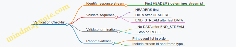
What You Should See in a Correct Run
A typical successful event sequence for a single request looks like:
HEADERS(response headers)- Zero or more
DATAframes (response body chunks) END_STREAM
If you see DATA before HEADERS, it usually means your callback is mixing streams or your event mapping is off. If you see DATA after END_STREAM, you likely logged events from multiple streams without filtering.
Practical Notes for Common Pitfalls
- Stream confusion: Always tag events with stream id and filter before verifying.
- Multiple HEADERS: Some implementations may emit additional header-related frames; if so, adjust Rule A to allow a second header-like event only when it is still semantically part of the response.
- Reset behavior: Treat
RESETas a terminal event and do not expectEND_STREAMafterward.
Run the verifier on every test request you send. When it fails, the event list becomes your map of what happened, not a mystery novel written in packet timing.
6. QPACK Behavior and Header Compression Optimization
6.1 QPACK Encoder and Decoder Roles with Dynamic Tables
QPACK is the header compression system used by HTTP/3. Its job is simple to state and subtle to implement: compress request and response headers while keeping the decoder from stalling the entire connection. The trick is splitting responsibilities between an encoder side and a decoder side, then coordinating them with a dynamic table that both sides can reference.
Core Roles and Division of Labor
On the encoder side, QPACK maintains a dynamic table that stores header fields for later reuse. When sending a header block, the encoder chooses either static table entries (predefined by the spec) or dynamic table entries (learned during the connection). The encoder then emits two kinds of information:
- Header blocks that carry compressed header representations.
- Dynamic table instructions that tell the decoder how to populate and index the dynamic table.
On the decoder side, QPACK receives header blocks and must map each reference to the correct table entry. If a header block references a dynamic entry that the decoder has not learned yet, the decoder cannot guess. Instead, QPACK provides a mechanism to wait efficiently without blocking unrelated streams.
Dynamic Tables as a Shared Index
A dynamic table is an ordered list of header fields. Each inserted field gets an index relative to the table’s current state. The encoder and decoder must agree on the sequence of insertions and evictions, otherwise an index would point to the wrong header field.
To keep this agreement, the encoder sends insert-with-indexing instructions. The decoder applies them in order, updating its own dynamic table. When the encoder later references an index in a header block, the decoder can resolve it deterministically.
Mind Map: QPACK Data Flow and Dependencies
How Encoding Works Step by Step
Consider a request with headers like :method GET, :path /video, and accept: video/mp4. The encoder typically:
- Uses the static table for well-known pseudo-headers.
- Chooses dynamic table entries for repeated or frequently used fields, such as
accept. - If it wants the decoder to use a dynamic entry, it first sends an instruction to insert that header field into the dynamic table.
- Sends the header block that references the dynamic index.
A key detail: the encoder does not have to wait for the decoder to process the instruction before sending the header block. That’s where QPACK’s coordination comes in.
How Decoding Works Step by Step
When the decoder receives a header block, it parses the representations and resolves each reference:
- Static references are resolved immediately.
- Dynamic references require the decoder’s dynamic table to already contain the referenced entry.
If the referenced dynamic entry is not yet available, the decoder must handle it without freezing everything. QPACK uses a controlled waiting mechanism so that only the affected stream’s decoding is delayed, while other streams can continue.
Example: Dynamic Table Insert and Reference
Suppose the encoder inserts accept: video/mp4 into the dynamic table. The decoder must learn this insertion before it can resolve a header block that references the resulting index.
Example:
- Encoder sends dynamic instruction: insert
accept: video/mp4. - Encoder sends header block: reference dynamic index for
accept: video/mp4. - Decoder applies instruction in its dynamic table.
- Decoder decodes header block using the dynamic index.
If the header block arrives first, the decoder cannot resolve the dynamic index yet. QPACK’s synchronization prevents incorrect decoding by forcing the decoder to wait for the missing dynamic table state.
Advanced Details That Matter in Practice
Ordering and Index Consistency
Dynamic table indices are only meaningful relative to the exact sequence of insertions and evictions. That means the decoder must apply instructions in the same order the encoder intended. If the decoder lags, it may temporarily lack entries, but it will not invent them.
Controlled Blocking
The system is designed so that waiting is localized. A stream that references an unavailable dynamic entry may pause, but other streams can still decode headers that rely only on static entries or already-known dynamic entries.
Why Two Channels Exist
QPACK separates header blocks from dynamic table instructions so that the decoder can receive instructions and apply them independently of stream scheduling. This separation reduces the chance that a single slow stream forces global stalling.
Quick Mental Model
Think of the dynamic table as a shared notebook page that the encoder writes into. Header blocks are like short notes that cite page numbers. If a note cites a page that hasn’t been written yet, the reader waits for that page—no guessing, no rewriting history.
Summary of Encoder and Decoder Responsibilities
- The encoder chooses which headers to store in the dynamic table and emits instructions plus compressed header blocks.
- The decoder maintains the dynamic table, resolves references during header decoding, and uses synchronization to handle cases where dynamic entries arrive later than the header blocks that reference them.
6.2 Acknowledgments and Insert With Acknowledgment Mechanics
QPACK splits header compression into two jobs: the encoder sends compressed header representations, and the decoder reconstructs them. The “acknowledgment mechanics” exist because the decoder may not yet have the dynamic table entries needed to interpret references. So the protocol uses explicit signals: the encoder can insert entries, and the decoder can acknowledge which inserts it has received and which references are now safe.
Core Idea: Why Acknowledgments Exist
In HTTP/3, header blocks travel on request and response streams. Dynamic table entries, however, are managed on separate control streams. That separation is useful for parallelism, but it means the decoder might see a header block that references an entry it has not learned yet. Acknowledgments let the encoder learn what the decoder knows, and they let the decoder avoid indefinite waiting.
A practical mental model: treat each dynamic table insert as a “dictionary update.” A header block can reference dictionary entries by index. If the decoder hasn’t received the dictionary update, it must either wait or fail the stream.
Insert Mechanics: What Gets Sent and When
An encoder sends dynamic table insert instructions on the encoder-to-decoder stream. Each insert is assigned an index in the dynamic table space. The decoder applies inserts in order, updating its dynamic table state.
Two details matter for correctness:
- Index stability: the decoder must apply inserts in the same order the encoder intended, so indices remain meaningful.
- Bounded memory: both sides enforce limits on dynamic table size, so inserts may evict older entries.
When the encoder emits a header block, it may reference dynamic table indices. If those indices correspond to inserts the decoder has not yet processed, the decoder must handle the gap.
Acknowledgment Mechanics: What the Decoder Sends Back
The decoder-to-encoder acknowledgment stream carries signals that describe which insert indices the decoder has received and processed. The encoder uses these acknowledgments to manage its own state and to decide how aggressively it can send future inserts.
A useful way to think about it:
- Decoder acknowledgments are a progress report for the dynamic table.
- Encoder insert scheduling is a pacing mechanism based on that progress.
This prevents the encoder from running far ahead of the decoder’s ability to apply inserts, which would otherwise increase the chance that header blocks reference missing entries.
Blocking Avoidance: How the Decoder Behaves
When a header block references an index not yet available, the decoder can enter a waiting state. The protocol provides a mechanism so the decoder can avoid deadlock by relying on the encoder’s inserts and the decoder’s own acknowledgment progress.
In practice, the decoder’s waiting is bounded by the protocol’s control flow:
- The decoder waits for the required inserts to arrive.
- The decoder continues to process control information so that inserts can be applied.
- If the required inserts never become available within the protocol’s constraints, the stream is reset.
This is why acknowledgments are not optional decoration; they are part of the control loop that keeps header decoding from stalling indefinitely.
Mind Map: Acknowledgments and Insert Flow
Example: A Missing Dynamic Index Reference
Assume the encoder sends:
- Insert entry #10 on the encoder-to-decoder stream.
- Immediately sends a header block referencing dynamic index #10 on the request stream.
If the request stream arrives before the insert stream update is processed, the decoder sees a reference to #10 that is not yet in its dynamic table. The decoder waits until it receives and applies the insert instruction for #10.
Now add acknowledgments:
- After applying #10, the decoder sends an acknowledgment indicating that #10 (and possibly earlier inserts) are processed.
- The encoder receives that acknowledgment and can safely schedule subsequent inserts and header blocks with fewer “wait for insert” events.
The key point is that the protocol doesn’t guess. It measures progress and uses that measurement to coordinate the two control planes.
Example: Insert Pacing to Reduce Decoder Waiting
Consider a workload with many short requests. If the encoder inserts a large batch of dynamic entries but the decoder lags, many header blocks may reference indices that are not yet ready. That increases waiting and can lead to stream resets under tight constraints.
A better approach is to pace inserts:
- Send a modest number of inserts.
- Wait for decoder acknowledgments that confirm those inserts are processed.
- Then send header blocks that rely on those indices.
This keeps the dynamic table “warm” at the decoder without forcing it to stall on every request.
Practical Checklist for Correctness
- Ensure insert indices referenced by header blocks correspond to inserts the decoder can reach.
- Treat decoder acknowledgments as the authority for decoder progress.
- Keep dynamic table limits consistent so indices don’t become invalid due to eviction.
- When debugging, correlate header-block arrival with insert processing order to explain waiting or resets.
Acknowledgments and inserts form a tight loop: inserts create dictionary entries, acknowledgments confirm their availability, and header blocks rely on that confirmed state. When the loop is respected, decoding stays orderly even when streams arrive out of sync.
6.3 Blocking Avoidance and Decoder Stream Constraints
QPACK’s job is to compress HTTP/3 headers without forcing the decoder to wait for the encoder’s future decisions. The main trick is to split header processing into two roles: the encoder sends instructions and the decoder applies them as soon as it can. When the decoder can’t apply an instruction yet, it must avoid stalling the entire connection. That’s where blocking avoidance and decoder stream constraints come in.
Core Idea: Keep Decoding Moving
In QPACK, the encoder maintains a dynamic table and emits updates. The decoder also maintains a dynamic table, but it learns updates via a dedicated control stream. If the decoder receives a header block that references dynamic table entries it hasn’t learned yet, it would normally have to wait. QPACK prevents unbounded waiting by using two mechanisms:
- A decoder stream for acknowledgments and requests so the encoder can learn what the decoder has consumed.
- Rules that limit how the decoder can request missing entries, ensuring the decoder doesn’t deadlock itself.
Decoder Stream Constraints: What They Prevent
The decoder stream is not a general-purpose channel. It exists to carry specific signals that let the encoder safely manage dynamic table state. The constraints are designed to avoid two failure modes:
- Head-of-line blocking at the connection level: if one stream stalls, other streams shouldn’t be forced to wait.
- Circular dependency between encoder and decoder: the decoder shouldn’t need the encoder to send something that the encoder can’t send until the decoder acknowledges it.
A practical way to think about it: the decoder can ask for entries, but it must do so in a bounded, ordered manner that the encoder can satisfy without waiting on the decoder’s future behavior.
Mind Map: QPACK Blocking Avoidance
Step-by-Step Flow: From Header Block to Safe Recovery
- Decoder receives a header block on an HTTP/3 request stream.
- The header block may reference dynamic table entries by index.
- If the decoder already has those entries, it decodes immediately.
- If not, it must determine whether it can request the missing entries without violating constraints.
- The decoder sends a signal on the decoder stream indicating what it needs.
- The encoder, upon receiving decoder stream signals, can transmit the required dynamic table updates on the encoder stream.
- Once the decoder receives and applies those updates, it can finish decoding the header block.
The key is that the decoder’s request is structured so the encoder can respond deterministically, rather than guessing which updates are safe to send.
Concrete Example: Missing Dynamic Entry Without Connection-Wide Stall
Imagine a client sends two HTTP/3 requests on different streams.
- Request A includes headers that reference dynamic table entry #12.
- Request B includes headers that reference dynamic table entry #20.
Suppose the decoder has learned up to entry #15 but not #20 yet. When decoding Request B, it can’t resolve #20 immediately.
Instead of pausing the entire connection, the decoder:
- Continues processing what it can for other streams.
- Sends a decoder stream signal requesting the missing entry range needed to resolve #20.
- Waits only for the specific dynamic table updates required for Request B.
This keeps the stall localized to the stream that needs the missing entry, which is the practical meaning of “avoid blocking.”
Advanced Detail: Why Ordering Matters
If the decoder were allowed to request arbitrary missing entries out of order, the encoder could be forced into sending updates that the decoder might never apply, or the system could end up waiting on acknowledgments that depend on updates that haven’t been sent. The constraints enforce an ordering discipline so that:
- The encoder’s dynamic table evolution remains consistent with what the decoder can eventually learn.
- The decoder’s requests correspond to a coherent prefix of dynamic table history.
In effect, the decoder stream acts like a “receipt lane” for progress, not a free-form instruction channel.
Practical Checklist for Implementers
- Ensure the decoder can identify when a referenced dynamic entry is unknown.
- Implement decoder stream signaling so requests are bounded and ordered.
- Make stream-level decoding behavior explicit: only the affected request stream should wait for missing entries.
- Confirm that encoder handling of decoder signals can advance dynamic table updates without requiring additional decoder actions that would create a cycle.
When these pieces line up, QPACK can compress headers efficiently while keeping decoding responsive, even when packets arrive out of order. The decoder stream constraints are what make that reliability possible without turning every header into a waiting game.
6.4 Tuning QPACK Settings for High-Latency Environments
QPACK sits between HTTP/3 headers and QUIC streams. It reduces header size by compressing repeated fields, but it also introduces a coordination problem: the decoder may need dynamic table entries that the encoder has not yet communicated. High latency makes that coordination more expensive, so tuning is mostly about controlling how often the decoder waits and how much state you allow to accumulate.
Core Mechanics You Tune
QPACK has two roles: the encoder sends instructions to build a dynamic table, and the decoder uses those instructions to interpret compressed header blocks. The key operational knobs are:
- Dynamic Table Capacity: how many entries the encoder can keep. Larger capacity improves compression when requests share header patterns, but it also increases the amount of state that must be synchronized.
- Stream Limits for QPACK Control: the number of streams used for encoder instructions and acknowledgments. More streams can reduce head-of-line effects between control traffic and header traffic.
- Acknowledgment Behavior: the decoder sends acknowledgments for received instructions. If acknowledgments lag, the encoder may be forced to wait before evicting or reusing indices.
- Blocking Avoidance Strategy: when the decoder references an index not yet known, it can block until the needed instruction arrives, or it can use a safer mode that trades compression efficiency for fewer stalls.
Mind Map: High-Latency QPACK Tuning
Step 1: Classify Your Header Patterns
Start with a simple observation: which headers repeat across requests from the same client or within the same service? If you mostly send stable headers like :method, :path prefixes, host, and a small set of application headers, a moderate dynamic table helps. If paths are highly unique, a large table mainly stores noise and increases synchronization cost.
Example: Suppose a CDN edge serves many requests where host and user-agent repeat, but :path varies per object. A smaller dynamic table still captures the repeated fields, while avoiding excessive churn from unique paths.
Step 2: Choose a Dynamic Table Capacity That Matches RTT
In high-latency networks, the decoder can be waiting for instructions longer than in low-latency networks. If the dynamic table is too small, you lose compression and send more literal headers. If it is too large, you increase the chance that the decoder references indices that are not yet available.
A practical approach is to set capacity so that the encoder can cover the working set of repeated headers for a short burst of concurrent requests.
Example: If you typically have 20 concurrent requests per connection and the repeated header set fits into about 200 distinct dynamic entries, start with a capacity near that scale. Then verify that blocked header blocks remain rare under induced delay.
Step 3: Reduce Decoder Blocking by Managing Instruction Flow
Decoder blocking happens when a header block references a dynamic table index that the decoder has not received. You can reduce this by ensuring the encoder sends the needed instructions early enough relative to header blocks.
Two tactics work well together:
- Pace encoder instructions so they are not delayed behind other QUIC traffic.
- Limit how aggressively you reuse indices when acknowledgments are slow.
Example: If you observe that header blocks frequently stall waiting for dynamic entries, slow down the rate at which you advance the dynamic table index for new entries. This keeps the decoder’s “known indices” closer to what the encoder references.
Step 4: Allocate Control Stream Concurrency Carefully
QPACK control traffic uses dedicated streams. With high latency, control streams can become bottlenecks if they share scheduling pressure with application streams.
- If your implementation supports it, allow enough control stream concurrency to prevent instruction and acknowledgment traffic from queueing behind each other.
- If you run many concurrent requests, ensure the control plane has room to keep up.
Example: A server handling 100 concurrent HTTP/3 requests per connection should not assume a single control stream will always stay ahead. If you see queueing in QPACK control streams, increase control stream concurrency or reduce per-connection request concurrency.
Step 5: Validate with Targeted Measurements
Tuning without measurement is just guessing with extra steps. Focus on three signals:
- Blocked Header Blocks Count: how many header blocks wait for missing dynamic entries.
- Time To First Decoded Header: the latency from header block arrival to successful decoding.
- QPACK Stream Queueing: whether control streams accumulate backlog.
Example: Run a controlled test with fixed RTT and induced jitter. Compare two configurations: one with smaller dynamic table capacity and one with larger capacity. The best choice is the one that minimizes blocked header blocks while keeping header size reasonable.
Practical Configuration Pattern
Use a conservative baseline for high-latency links: moderate dynamic table capacity, sufficient control stream concurrency, and instruction pacing that avoids referencing indices too far ahead of what the decoder can learn.
Example: For a connection profile with long RTT and bursty request concurrency, start with a dynamic table sized for the repeated header working set, then adjust upward only if blocked header blocks stay near zero and header size meaningfully decreases.
6.5 Trace-Based Debugging of QPACK Blocking and Recovery
QPACK blocking happens when the decoder needs header entries that the encoder has not yet made available. Recovery is the process by which the connection eventually supplies the missing dynamic table state so decoding can continue. Traces let you see both sides: what the decoder asked for, what the encoder promised, and when the protocol’s flow-control mechanisms allowed progress.
What to Look for First
Start with the HTTP/3 stream timeline. Identify the request/response header block stream and the QPACK control streams (encoder stream and decoder stream). Then locate the moment decoding stalls: the decoder has received a header block fragment but cannot map some dynamic table references.
In a trace, the stall usually shows up as:
- Header block fragments arriving without corresponding “decoded header fields” progress.
- QPACK instructions that arrive late relative to the header block.
- A gap between decoder stream acknowledgments and encoder stream inserts.
A useful mental model is a two-lane system: header blocks travel on one lane, while dynamic table updates travel on another. Blocking occurs when the header lane outruns the table lane.
Mind Map of Blocking and Recovery Signals
QPACK Blocking and Recovery Mind Map
Step-by-Step Trace Workflow
-
Mark the header block boundaries. Find the first header block fragment for a response (or request). Record the stream ID and the approximate packet number.
-
Extract QPACK instructions around the stall. In the same time window, capture QPACK frames on the control streams. You are looking for two categories: dynamic table inserts and acknowledgments.
-
Match dynamic table references. When the decoder blocks, it is typically waiting for a specific dynamic table entry index or a reference tied to an instruction sequence. In the trace, correlate the blocked header block with the later arrival of the insert that would have populated that entry.
-
Check instruction sequence ordering. QPACK uses instruction sequence numbers to coordinate availability. If you see inserts arriving after the header block references, blocking is expected. If inserts never arrive, the issue is usually flow control or stream cancellation.
-
Confirm recovery completion. Recovery is not “frames arrived”; it is “decoding progressed.” Look for the point where the decoder can finish the header block and the application receives the decoded fields.
Concrete Example: Decoder Waits for Missing Inserts
Assume a client sends a request with multiple header blocks on a single HTTP/3 connection. The trace shows:
- Packet A: header block fragment arrives on stream 7.
- Packet B: decoder cannot resolve a dynamic table reference and pauses.
- Packet C: encoder inserts dynamic table entries but they arrive after the pause.
- Packet D: decoder receives the insert and resumes decoding.
How to verify this is QPACK blocking rather than a generic transport issue:
- The stall aligns with QPACK control frames, not with general packet loss.
- The missing dynamic entries appear shortly after, and decoding resumes without a connection error.
If you also see decoder acknowledgments earlier than the corresponding inserts, that can still be normal. Acknowledgments indicate the decoder has processed some instruction sequence numbers; they do not guarantee that every referenced entry for the current header block is already present.
Concrete Example: Flow Control Deadlock Symptoms
A different pattern suggests flow control problems:
- Header blocks keep arriving.
- QPACK inserts stop or arrive only partially.
- Decoder acknowledgments do not lead to new inserts.
In traces, this often looks like repeated header block fragments with no decoding progress, while control streams show limited forward movement. The practical check is to compare:
- The encoder’s ability to send inserts against its configured limits.
- The decoder’s consumption of dynamic table state.
If inserts are constrained, the decoder may keep waiting for entries that cannot be produced until the encoder’s control stream can advance.
Debugging Checklist You Can Apply Immediately
- Stream mapping: Confirm you are reading the correct header block stream and the correct QPACK control streams.
- Temporal ordering: Determine whether the header lane outran the table lane.
- Instruction correlation: Match blocked dynamic references to the later insert instruction sequence.
- Recovery marker: Identify the packet where decoding completes, not just where frames arrive.
- Error vs stall: Distinguish “waiting” from “reset or termination,” since resets change the interpretation of missing frames.
When you follow this workflow, QPACK blocking becomes a traceable cause-and-effect chain: decoder requests what it needs, encoder supplies it when allowed, and decoding resumes when the dynamic table state catches up.
7. Transport Parameterization and Negotiation
7.1 Transport Parameters and Their Negotiated Meaning
Transport parameters are the knobs QUIC uses to agree on how the connection will behave before application data starts flowing. They are carried during the handshake, then treated as hard constraints by both endpoints. Think of them as “rules of the road” that prevent one side from assuming unlimited resources while the other side assumes strict limits.
What Gets Negotiated and Why It Matters
Transport parameters include limits and timers that directly affect reliability, buffering, and connection lifetime. Examples include maximum stream counts, flow-control limits, idle timeout, and the maximum datagram size when datagrams are used. Because these values influence how much state an endpoint must allocate and how aggressively it can send, negotiation is not just informational; it determines correctness.
A practical way to see the impact: if the client believes it can open more streams than the server will allow, the client will eventually hit a limit and must handle stream errors. Negotiated parameters reduce that mismatch by making the limit explicit.
Handshake Timing and the “Before Data” Contract
Transport parameters are exchanged during the handshake, so both sides can apply them before sending application data that depends on them. This ordering matters for two reasons.
First, it avoids mid-flight renegotiation of core limits that would otherwise require complex rollback. Second, it keeps loss recovery and flow control consistent: the sender’s pacing and the receiver’s buffering expectations are aligned from the start.
Interpreting Negotiated Values Correctly
Negotiated meaning is not always “take the peer’s number.” For many parameters, the effective behavior is the minimum of what both sides are willing to support. For example, if the client advertises a maximum stream count of 100 and the server advertises 50, the connection must behave as if the maximum is 50. This “min rule” prevents the sender from exceeding what the receiver can safely track.
Some parameters are instead interpreted as the sender’s capability that the receiver can rely on. For instance, when a maximum datagram size is negotiated, the sender must not exceed it because the receiver may not be able to process larger datagrams.
Mind Map: Transport Parameters and Their Effects
Worked Example: Stream Limits in Action
Assume the server sets:
- max bidirectional streams = 50
- max unidirectional streams = 20
The client sets:
- max bidirectional streams = 80
- max unidirectional streams = 10
Effective limits become:
- bidirectional streams = min(50, 80) = 50
- unidirectional streams = min(20, 10) = 10
If the client tries to open 60 bidirectional streams, it violates the negotiated contract and should expect a stream-related error rather than silent failure. The key point is that the client’s own advertised number does not grant extra capacity; the peer’s constraints cap it.
Worked Example: Idle Timeout and Keepalive Behavior
Suppose the server advertises an idle timeout of 30 seconds. If the connection sees no packets for longer than that, the server may close it. The negotiated meaning is operational: the client must ensure it sends something within the timeout window if it needs the connection to remain active.
A simple test scenario is to run a client that sends one request, then waits. If the server closes after ~30 seconds of silence, the behavior matches the negotiated idle timeout rather than any local guesswork.
Implementation Notes That Prevent Subtle Bugs
- Treat negotiated parameters as constraints, not hints.
- Apply the correct combination rule per parameter: min for shared limits, strict respect for capability bounds.
- When debugging, correlate application symptoms with the negotiated values from the handshake rather than with local defaults.
Mind Map: Effective Value Calculation
Example: A Minimal Negotiation Checklist
Before sending application data that depends on limits, verify:
- The handshake completed successfully.
- The negotiated stream limits are recorded.
- The idle timeout is known if you expect long pauses.
- If datagrams are used, the maximum datagram size is respected.
That checklist sounds boring, which is exactly why it works: most transport bugs come from assuming defaults that were never negotiated.
7.2 Limits for Streams and Flow Control with Practical Selection Guidance
QUIC gives you two knobs that strongly shape performance: stream limits (how many concurrent streams you allow) and flow control limits (how much data each side is permitted to send). If you set them too low, you throttle yourself. If you set them too high, you invite buffer bloat and long recovery times when loss happens. The trick is to choose limits that match your workload’s concurrency and its tolerance for backpressure.
Core Concepts That Drive Limit Choices
Start with the mental model: HTTP/3 carries requests and responses over QUIC streams, and QUIC flow control gates how much stream data can be in flight. QUIC has two layers of flow control: connection-level flow control caps the total bytes outstanding across all streams, while stream-level flow control caps bytes outstanding per stream. Stream limits cap how many streams can exist concurrently in each direction.
A practical consequence: even if you allow many streams, a small connection-level limit can still prevent progress because all streams share the same total budget. Conversely, a large connection-level limit with tiny stream-level limits can cause each stream to trickle data slowly, which is especially noticeable for large responses.
Selecting Stream Limits for Real Workloads
Stream limits should reflect how many independent units of work you expect at once. For HTTP/3, that usually maps to concurrent requests per client connection.
Use this rule of thumb:
- If your workload is request/response with short bodies, you can support more concurrent streams because each stream finishes quickly.
- If your workload includes large uploads or downloads, fewer concurrent streams often yields better responsiveness because flow control updates and loss recovery have less contention.
A concrete example: a client that fetches 20 small JSON documents in parallel can benefit from a higher stream limit. A client that uploads 5 large files concurrently may perform better with a lower stream limit, because each upload consumes stream-level and connection-level flow control budgets for longer.
Selecting Flow Control Limits for Throughput Without Bloat
Flow control limits should be large enough to keep the pipe moving, but not so large that you accumulate excessive queued data when the network misbehaves.
Think in terms of “in-flight bytes” during steady state. If your effective bandwidth is B bytes/second and your typical round-trip time is RTT seconds, then a rough target for in-flight bytes is B × RTT. QUIC flow control should allow at least that amount so the sender can keep transmitting while waiting for acknowledgments.
Now add loss and jitter reality: when packets are lost, the sender may continue transmitting until it hits flow control limits, and then it must wait for acknowledgments and recovery. Larger limits can hide some stalls, but they also increase the amount of data that may need retransmission.
A practical selection workflow:
- Estimate your typical RTT range and peak throughput.
- Compute a baseline in-flight target (B × RTT).
- Add headroom for burstiness in application writes.
- Cap concurrency so that the sum of per-stream needs does not exceed the connection-level budget.
Integrated Example with Numbers
Assume a client link that averages 5 MB/s with an RTT of 80 ms. The baseline in-flight target is:
- 5,000,000 bytes/s × 0.08 s = 400,000 bytes
If you set connection-level flow control to 400 KB, you may see underutilization when bursts occur or when acknowledgments arrive late. A reasonable starting point is to allow about 2× the baseline for connection-level flow control, such as 800 KB, while keeping stream-level limits aligned with typical response sizes.
For stream-level limits, consider a common case: small responses around 50 KB. If you set stream-level flow control to 64 KB, each stream can send its body with minimal waiting. For large responses, you can either raise stream-level limits or rely on incremental sending, but you should ensure that the connection-level limit can accommodate multiple large streams without stalling.
Mind Map: Stream and Flow Control Limit Selection
Validation Checklist That Prevents “It Works on My Network”
After choosing limits, validate behavior under two conditions: normal operation and mild impairment. Normal operation confirms you are not artificially throttling. Mild impairment confirms you do not create excessive queued data that slows recovery.
A simple test pattern:
- Run a workload with your expected concurrency.
- Observe whether streams stall waiting for flow control updates.
- Check whether loss causes large retransmission bursts that correlate with oversized flow control.
If you see frequent stalls, increase the relevant limit (connection-level if many streams compete; stream-level if single large streams crawl). If you see large retransmissions and long recovery, reduce headroom or concurrency so the sender cannot accumulate too much outstanding data.
The goal is not to maximize numbers. It is to keep the sender busy when the network is healthy and to keep the outstanding data bounded when it is not.
7.3 Idle Timeout, Keepalive Behavior, and Connection Longevity
QUIC connections are designed to stay useful even when traffic pauses. That said, “idle” is not a single universal state: different layers (QUIC, HTTP3, NATs, load balancers) each have their own ideas about when a path is no longer worth keeping. The goal of this section is to make those ideas concrete so you can choose timeouts and keepalive behavior that match your network reality.
Idle Timeout Fundamentals
An idle timeout is the maximum time a connection can remain without receiving or sending data before the endpoint closes it. In QUIC, “data” is not limited to application payload; it includes protocol packets that keep the connection alive in a meaningful way.
A practical way to reason about it is to separate two clocks:
- Local activity clock: how long since your endpoint last sent or received QUIC packets.
- Path viability clock: how long the network path (often via NAT state) will keep forwarding packets.
If your local idle timeout is shorter than the path viability clock, you close first and lose the benefit of keeping the connection around. If your local idle timeout is longer, the network may silently drop state, and the next packet you send may fail until you re-establish.
Example: Choosing an Idle Timeout for a Chat App
Suppose a chat client sends a message, then waits 30 seconds for a reply. If you set an idle timeout of 10 seconds, the connection will close during normal pauses. If you set it to 5 minutes, the connection likely survives typical pauses, but you must ensure the server can handle many long-lived idle connections without exhausting resources.
A good starting point is to set the idle timeout slightly above the 95th percentile of your observed inter-message gap, then validate with traces.
Keepalive Behavior
Keepalives are packets sent when there is no application data to send. In QUIC, keepalives are typically implemented using small frames that do not carry application semantics but still count as QUIC traffic.
The important nuance is that keepalives must be frequent enough to beat the smallest relevant timeout in the chain. That chain can include:
- NAT binding timeouts
- Firewall session timeouts
- Load balancer idle timers
- QUIC endpoint idle timeout
Example: Keepalive Interval vs NAT Timeout
If a NAT mapping tends to expire after 30 seconds of inactivity, sending a keepalive every 20 seconds gives you margin. Sending every 35 seconds might work on some networks and fail on others, which is the worst kind of “works on my machine.”
Keepalive Cost Accounting
Keepalives consume bandwidth, CPU, and packet processing overhead. They also create more events in your observability pipeline. A useful rule is to keep keepalives rare but reliable: pick an interval that is comfortably below the most constrained timeout you observe, then measure the resulting packet rate.
Connection Longevity and Resource Management
Long-lived connections are not free. Even when idle, they occupy state: cryptographic context, stream bookkeeping, flow-control limits, and congestion control variables. Longevity is therefore a balancing act between:
- User experience: fewer handshakes and faster resumption of streams
- Operational stability: bounded memory and file descriptors
Practical Strategy: Tiered Lifetimes
Instead of one global “forever” policy, use tiered behavior:
- Short idle timeout for low-value connections: e.g., connections that only serve infrequent requests.
- Longer idle timeout for high-value sessions: e.g., interactive clients that frequently resume.
This can be implemented by configuring different server endpoints or by applying policy based on request patterns.
Mind Map: Idle Timeout, Keepalive, Connection Longevity
Example: A Systematic Tuning Workflow
- Measure inter-arrival gaps for your traffic. Compute a distribution of time between meaningful requests.
- Measure network idle constraints by observing when connections break during inactivity in your target environments.
- Set idle timeout slightly above your typical long pause window, but keep it below the point where you see widespread “next packet fails” behavior.
- Set keepalive interval to beat the smallest observed network timeout with margin.
- Validate with traces by checking whether connections remain open across idle gaps and whether the first post-idle packet arrives without requiring a new handshake.
If you follow this sequence, you end up with timeouts that are justified by data rather than guesswork. The connection stays alive when it should, and it closes when it must—no more, no less.
7.4 Version Negotiation and Compatibility Handling
Version negotiation is the part of QUIC that prevents “almost compatible” endpoints from wasting time. When a client and server disagree on the QUIC version, the server can respond with a version list, and the client can retry using a mutually supported version. HTTP/3 sits on top of QUIC, so version compatibility also affects how HTTP/3 parameters are interpreted and how errors are surfaced.
Core Concepts That Drive Compatibility
QUIC version negotiation happens before the connection is fully established. The client sends an Initial packet that includes a version field. If the server does not support that version, it replies with a Version Negotiation packet containing supported versions. The client then selects one and sends a new Initial packet.
Compatibility is not only about “which version number.” It also includes:
- Transport parameters interpretation: the meaning and limits of parameters can vary by version.
- Packet format expectations: fields like packet number length, header layout, and integrity coverage must match.
- HTTP/3 mapping: HTTP/3 frames ride inside QUIC streams, but the transport version determines how those streams are carried and how errors are encoded.
Mind Map: Version Negotiation Flow
Step-by-Step Negotiation with Concrete Example
Imagine a client configured for QUIC version 1 and a server that only supports version 2. The client sends an Initial packet with version 1. The server cannot proceed because it does not implement version 1 packet semantics. Instead of pretending, it sends a Version Negotiation packet listing versions it supports.
The client receives the list and picks version 2. It then sends a fresh Initial packet using version 2. Only after the server accepts the version does the handshake proceed to key establishment and transport parameter negotiation.
A practical detail: the client should treat the first attempt as failed for transport-layer reasons, not as an HTTP/3 error. HTTP/3 request logic should start only after QUIC is ready to carry streams reliably.
Compatibility Handling Beyond Version Numbers
Once versions match, endpoints still need to agree on transport parameters. If the client proposes limits that the server cannot honor, the server can close the connection with an error that indicates parameter incompatibility. This is where “compatibility” becomes operational.
Key handling rules that keep behavior predictable:
- Fail fast on version mismatch: do not attempt to interpret frames or parameters from a mismatched transport.
- Validate transport parameters early: check stream limits and flow control constraints before relying on them for HTTP/3 concurrency.
- Keep HTTP/3 error mapping consistent: if QUIC closes during setup, the HTTP/3 layer should report a transport/setup failure rather than a malformed request.
Mind Map: Compatibility Decision Points
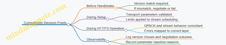
Example: Client Retry Strategy
A robust client keeps a small set of candidate versions and retries only when the server explicitly requests negotiation. The goal is to avoid repeated retries that look like network flakiness.
1. Send Initial with configured version Vc
2. If Version Negotiation received:
   a. Parse supported versions Vs
   b. Select V = first supported version in preference order
   c. Send new Initial with version V
3. If no overlap:
   a. Surface transport setup failure
   b. Do not attempt HTTP/3 requests
Example: Parameter Mismatch After Version Match
Suppose the client and server agree on QUIC version, but the client proposes a stream limit that exceeds what the server is willing to allocate. The server rejects the connection during setup. The HTTP/3 layer should not try to send requests on streams that the transport will never allow.
A clean implementation logs the rejection at the transport layer and returns an error to the caller that clearly indicates setup failure. The caller can then decide whether to retry with different transport settings.
Case Study: Mixed Environment with Two Server Pools
Consider a deployment where some servers support QUIC version 1 and others support version 2. A client configured for version 1 connects successfully to pool A. When it reaches pool B, it receives a Version Negotiation packet and retries with version 2. After that, HTTP/3 requests proceed normally.
The important compatibility behavior is that the client does not treat the first attempt as an HTTP/3 problem. It treats it as a transport negotiation step, which keeps error handling accurate and prevents confusing “bad request” reports when the real issue is “wrong transport version.”
7.5 Example: Selecting Parameters for a Target Network Profile
Suppose you run an HTTP/3 service for two user groups: (1) mobile users on LTE with frequent short outages, and (2) enterprise users on stable Wi‑Fi with occasional congestion. You want one QUIC configuration that behaves predictably, not one that “feels fast” in a lab and then trips over real networks.
Step 1: Start with a Network Profile That You Can Measure
Pick a target profile using concrete observations: typical RTT, RTT variance, loss rate, and whether loss is bursty. For instance, a reasonable LTE profile might be 80–120 ms RTT with occasional 1–3% burst loss and brief path changes. A stable Wi‑Fi profile might be 20–40 ms RTT with low loss but periodic queueing.
Step 2: Map Profile Signals to QUIC Parameters
QUIC behavior is shaped by transport parameters and implementation choices. The key is to set limits so the connection can make progress under stress while avoiding excessive buffering.
- Flow control limits: If you set connection and stream flow control too low, you throttle yourself during recovery. If you set them too high, you risk large queues that increase latency. A practical approach is to size flow control to cover at least one bandwidth-delay product worth of data per active stream class.
- Idle timeout and keepalive: Short outages can cause silent stalls if the connection waits too long. Too aggressive keepalives waste packets. Choose an idle timeout that exceeds typical inactivity gaps but is shorter than the longest expected “radio silence” window.
- Stream limits: If you allow too many concurrent streams, you can spend recovery and scheduling effort on work that doesn’t matter. If you allow too few, you force head-of-line behavior at the application level.
Step 3: Choose Values Using a Worked Example
Assume the LTE profile: RTT ≈ 100 ms, effective throughput during steady state ≈ 5 Mbps, and burst loss occurs during handovers.
- Compute a baseline bandwidth-delay product: 5 Mbps × 0.1 s = 0.5 Mb ≈ 62.5 KB.
- Set stream flow control: If your workload uses a small number of concurrent request/response streams, set per-stream flow control to cover multiple RTTs of data for that stream class. For example, 4×BDP ≈ 250 KB per stream.
- Set connection flow control: If you expect up to 16 concurrent streams, connection flow control should cover at least the sum of those stream budgets, with headroom for recovery. A conservative starting point is 16 × 250 KB = 4 MB, then add headroom for retransmissions; 6–8 MB is a common range for “works without surprises” behavior.
- Set stream concurrency: If your HTTP/3 clients typically open 6–12 streams concurrently, set the server’s maximum streams to something comfortably above that, such as 32, so you don’t reject legitimate concurrency during recovery.
- Set idle timeout: For LTE, a starting point might be around 30 seconds, because it tolerates normal pauses while still cleaning up dead connections. If your application has long-lived but quiet sessions, increase it; if it’s mostly request/response, keep it moderate.
Step 4: Validate with a Trace-Driven Checklist
Run the same workload under emulated conditions and check three things: (1) you never hit flow control limits during normal operation, (2) recovery completes without excessive queueing, and (3) the connection doesn’t churn due to timeouts.
- If you see frequent stalls where the sender waits for flow control, increase stream or connection limits.
- If you see rising latency after loss, reduce buffering by lowering flow control or limiting concurrent streams.
- If you see repeated connection re-establishment after brief inactivity, shorten idle timeout or add application-level keepalive behavior.
Mind Map: Parameter Selection Workflow
Example: Two Profiles, One Configuration Strategy
If you must support both LTE and Wi‑Fi with one configuration, base your flow control on the worse RTT profile (LTE) so you don’t throttle during recovery. Then cap concurrency so Wi‑Fi doesn’t accumulate too much queued data. In practice, that means: size flow control for LTE BDP, but keep stream concurrency moderate and rely on HTTP/3 stream scheduling to keep interactive responses from waiting behind bulk transfers.
Example: A Simple Decision Table
| Observation in Tests | Likely Cause | Parameter to Adjust |
|---|---|---|
| Sender pauses often | Flow control too tight | Increase stream or connection limits |
| Latency spikes after loss | Excess buffering | Reduce flow control or concurrency |
| Connections drop after quiet periods | Idle timeout too short | Increase idle timeout or add keepalive |
| Too many rejected streams | Stream limit too low | Raise max streams |
This example approach keeps the selection grounded: compute budgets from RTT and throughput, set limits that cover recovery without creating huge queues, and confirm with trace-based checks that match what you actually observe.
8. Handling High-Latency Networks and Long RTT Effects
8.1 RTT Budgeting for Handshake, Setup, and Application Data
RTT budgeting is the art of accounting for how many round trips your connection needs before useful bytes arrive, and how much time you spend waiting after that. In QUIC and HTTP/3, the “budget” is not just a single number; it’s a sequence: handshake, transport setup, then application data delivery. If you measure and plan those phases separately, you can make targeted changes instead of guessing.
Mind Map: RTT Budget Components
Phase 1: Handshake and Key Availability
A clean mental model starts with “when do encryption keys exist for the bytes I care about?” In a typical full handshake, the client sends Initial packets, the server responds, and only after the handshake completes can the client confidently send application data that the server can decrypt and process. That means your first useful application bytes are gated by at least one full RTT worth of timing in the common case.
With 0-RTT, the client may send early application data before the handshake finishes. The trade is that early data can be rejected, and the server must be prepared to handle replay safety rules. For budgeting, treat 0-RTT as “possibly useful bytes,” not “guaranteed useful bytes.” A practical way to keep the budget honest is to record two timings: time-to-first-decryptable-response and time-to-first-accepted-application.
Phase 2: Transport Setup and Negotiated Readiness
Even after keys exist, the connection still needs transport-level readiness. QUIC transport parameters and limits determine how quickly streams can start and how much data can be in flight. If your application assumes it can open many streams immediately, but the negotiated limits are tight, you’ll see a delay that looks like “mysterious latency” even though the handshake is already done.
HTTP/3 adds another setup layer: QPACK coordination. Headers are compressed, and the decoder may need dynamic table entries that arrive via dedicated streams. When those entries aren’t available yet, the decoder can block header processing until it receives the required information. In budgeting terms, this is a “setup-to-header-availability” gap that can be larger than you expect on high-latency paths.
Phase 3: Application Data and Delivery Timing
Application data delivery has its own gates: stream creation, flow control, and loss recovery. QUIC avoids head-of-line blocking across streams, but it still has ordering within a stream. If your request headers and body share a stream, the body can’t be processed until headers are parsed, and any retransmissions on that stream delay progress.
To budget application data, separate “bytes sent” from “bytes processed.” A connection can transmit quickly but still deliver late if acknowledgments are delayed, if loss detection triggers retransmissions, or if flow control limits force the sender to pause.
Example: Budgeting a Simple Request-Response
Assume a client connects to an HTTP/3 server over a path with RTT = 120 ms.
- Handshake phase: full handshake completes after roughly 1 RTT before application data is reliably usable. Budget: ~120 ms.
- Transport setup: stream limits and QPACK coordination add a small additional delay. Budget: ~10–30 ms in a healthy case.
- Application phase: request headers arrive, server processes, then response headers arrive. Even with good pipelining, expect another RTT-like component for request-to-response header availability. Budget: ~120 ms.
A reasonable first-byte estimate becomes ~250–270 ms for response headers, plus any extra time for response body pacing under flow control.
Now consider a high-loss variant where the first response packet is lost. Loss recovery can add another RTT-sized penalty depending on when loss is detected and how quickly retransmissions are scheduled. The budget should therefore include a “loss contingency” term rather than assuming a loss-free path.
Measurement: Turning Budgets into Numbers
To make this systematic, instrument three timestamps in your client and server logs:
- T0: time the client sends Initial packets.
- Tkeys: time application encryption keys are available for the relevant direction.
- Tfirst: time the application observes the first processed response bytes (not merely received packets).
Then compute:
- Handshake-to-keys = Tkeys − T0
- Keys-to-first = Tfirst − Tkeys
If Keys-to-first is large, the issue is usually transport setup (limits, QPACK blocking) or application processing, not the cryptographic handshake.
Optimization Levers That Match the Budget
- If handshake dominates, reduce round trips by using session resumption where appropriate and by ensuring early data is only used when replay safety and server behavior are compatible.
- If setup dominates, map headers and streams to avoid QPACK blocking and avoid opening more streams than your negotiated limits allow.
- If application dominates, tune packetization and avoid oversized writes that increase fragmentation risk; also design stream usage so critical headers are not delayed behind large bodies.
A good RTT budget ends up being a checklist: handshake phase, setup phase, application phase, and a loss contingency. When you can point to which bucket is large, you can fix the right thing without changing everything at once.
8.2 Impact of Loss, Reordering, and ACK Delays on Recovery
QUIC recovery is a balancing act between “I’m missing something” and “I’m sure I’m missing something.” Loss, reordering, and ACK delays each push that balance in different directions, and the side effects show up as different recovery patterns: earlier retransmissions, later retransmissions, or retransmissions that are technically correct but operationally wasteful.
Loss Detection Foundations
QUIC tracks packet numbers and uses acknowledgments to infer which packets arrived. When a packet is declared lost, QUIC can retransmit the frames it carried. The key detail is that loss detection is not instantaneous; it depends on how many newer packets have been observed and on timing rules. That means the same network event can produce different recovery timing depending on traffic rate and packet spacing.
Practical mental model:
- Loss creates gaps in packet number coverage.
- Reordering creates gaps temporarily, but they may later fill.
- ACK delays postpone the moment the sender learns about either gaps or fills.
Loss: When the Sender Should Retransmit
Loss is the cleanest signal: if packet N is missing and enough later packets are received, QUIC marks N lost and retransmits.
Example:
- Sender transmits packets 10–20.
- Packets 13 and 16 are dropped.
- By the time the sender has received packets far enough ahead, it marks 13 and 16 lost.
- Frames inside those packets are retransmitted on new packets, and the receiver can reconstruct the stream once the missing frames arrive.
What to watch: retransmission count and “recovery latency,” meaning the time from first loss to the first retransmitted packet that carries the missing frames.
Reordering: Correctness Without Premature Retransmission
Reordering means packets arrive out of order. QUIC’s loss detection tries to avoid declaring a packet lost just because it hasn’t shown up yet.
Example:
- Packets 30, 31, 32 arrive.
- Packet 33 is delayed in the network.
- Packets 34–36 arrive before 33.
- If the sender’s loss detection threshold is too aggressive, it may mark 33 lost even though it will arrive shortly after.
That leads to “unnecessary retransmissions”: the receiver will accept both the original and the retransmitted frames, but the sender spent bandwidth and the receiver spent processing to handle duplicates.
Operational nuance: reordering is often correlated with multipath routing, load balancing, or queueing differences across paths. Even when the network is healthy, reordering can look like loss until acknowledgments arrive.
ACK Delays: The Learning Problem
ACK delay affects when the sender learns what the receiver has received. QUIC can’t mark a packet lost based on knowledge it doesn’t have.
Example:
- Packet 50 is dropped.
- The receiver receives packets 51–60 but waits before sending ACKs.
- The sender continues transmitting new packets without learning that 50 is missing.
- Loss detection and retransmission are delayed because the sender’s “received coverage” view is stale.
This produces a different failure mode than reordering: fewer unnecessary retransmissions, but slower recovery. For real-time streams, slower recovery can mean missing deadlines even if the connection eventually recovers.
Combined Effects: How the Three Signals Interact
Loss, reordering, and ACK delays can stack in ways that change the recovery shape.
- Recovery Signals
- Loss
- Missing packet numbers
- Loss detection threshold triggers
- Retransmit missing frames
- Reordering
- Temporary gaps in packet numbers
- Threshold must be tolerant
- Risk of unnecessary retransmissions
- ACK Delays
- Sender learns later
- Loss detection delayed
- Recovery slower but often less wasteful
- Loss
- Recovery Outcomes
- Fast recovery
- Requires timely ACKs
- Works best when loss is clear
- Wasteful recovery
- Caused by reordering + aggressive thresholds
- Slow recovery
- Caused by ACK delays + loss
- Fast recovery
Concrete Walkthrough with Packet Numbers
Consider a sender transmitting packets 100–110.
- Packet 103 is lost.
- Packet 106 is reordered and arrives late.
- ACKs are delayed by the receiver.
Timeline sketch:
- Sender sends 100–110.
- Receiver receives 100–102, 104–105, 107–110.
- Receiver does not send ACK immediately.
- When ACKs finally arrive, the sender learns:
- 103 is missing for real.
- 106 arrived, so it was not truly lost.
Result:
- 103 is retransmitted.
- 106 is not retransmitted, avoiding waste.
- Recovery is slower than it would be with prompt ACKs.
Practical Validation: What to Measure
To reason about recovery behavior, measure three things together:
- Time to First Retransmission: how quickly missing frames reappear.
- Retransmission Rate: how often frames are resent.
- Duplicate Acceptance at Receiver: whether retransmissions were unnecessary.
Example checklist for a trace review:
- Identify packet gaps and when they become “declared lost.”
- Compare the arrival time of late packets to the sender’s loss declaration time.
- Compare ACK emission timing to the sender’s retransmission timing.
Key Takeaways for Tuning Decisions
- Loss drives retransmission correctness; reordering drives retransmission economy.
- ACK delays primarily drive retransmission timing, not correctness.
- The best recovery behavior comes from aligning loss detection sensitivity with the expected reordering and ACK behavior of the path.
In short: loss tells you what’s missing, reordering tells you what might be missing, and ACK delays tell you when you’ll know which one it is. QUIC’s recovery logic has to treat all three as first-class citizens, not just “packet loss with extra steps.”
8.3 Strategies for Reducing Effective Latency Without Speculation
Effective latency is what users feel: the time from “I want data” to “I can act on it.” In QUIC and HTTP/3, you can’t remove physics, but you can reduce the time spent waiting on avoidable stalls. The key is to separate latency into components—handshake setup, request/response scheduling, header processing, loss recovery, and application backpressure—then remove the biggest contributors with concrete, measurable changes.
Mind Map: Effective Latency Components and Fixes
Reduce Setup Latency with Connection Reuse
If a client repeatedly creates new connections, it pays setup cost every time. Reuse is the simplest win: keep a small pool of active HTTP/3 connections per origin and reuse them for multiple requests. When resumption is available, prefer it for repeat clients so the handshake path is shorter. For 0-RTT, treat it as “fast path with strict rules”: only send idempotent operations or operations that can tolerate replay without changing state. A practical pattern is to use 0-RTT for fetching cached or read-only resources, and fall back to a normal request when the server indicates it cannot safely accept early data.
Example: A client fetches a user profile and a list of recent items. The profile is safe to replay, so it can be sent on 0-RTT. The “mark notifications as read” action is not safe, so it waits for handshake confirmation.
Reduce Scheduling Latency with Stream Timing and Isolation
Even with a fast network, latency grows when your important stream waits behind work that doesn’t matter. HTTP/3 multiplexes streams over one connection, so you control ordering by how you create streams and how you structure responses.
First, create the “latency-sensitive” stream early. If you know you need a small response to render a page, start that request immediately rather than batching it behind larger downloads. Second, isolate large transfers: avoid sending a huge response on the same connection at the same time as a critical interactive request unless you have a clear prioritization strategy. Third, keep concurrency intentional. Too little concurrency causes idle time; too much can increase queueing and flow-control pressure.
Example: A client starts a small JSON configuration request, waits for it, then begins downloading a large media segment. If you must overlap, ensure the small request is not queued behind the large one in your application’s send loop.
Reduce Processing Latency with QPACK Discipline
Header compression can help throughput, but it can also introduce waiting. QPACK uses dynamic tables and separate encoder/decoder behavior; the decoder may block if it needs entries that haven’t arrived yet.
To reduce effective latency, keep headers small and predictable for early responses. Avoid sending unusually large header sets on the critical path. Also, structure responses so that the first response headers are likely to be decodable without waiting on late dynamic table updates. On the server side, choose QPACK settings that match your environment: in high-latency networks, you want enough capacity to prevent the decoder from stalling, but not so much that you create excessive churn.
Example: Instead of sending a long cookie header on every request, use a smaller session token and move bulky metadata into a later request. The first response becomes decodable sooner, even if total bytes are similar.
Reduce Network-Induced Latency with Faster, Smarter Recovery
Loss recovery is a major source of “mysterious” delay. QUIC detects loss using packet number spaces and timing, then retransmits. You can’t retransmit before you know something is missing, but you can reduce the time until detection and the time until the retransmitted data is usable.
Practical steps:
- Keep packet sizes aligned with the path MTU to reduce fragmentation and loss.
- Avoid sending bursts that exceed the congestion window; they increase loss probability and trigger recovery.
- Ensure acknowledgment behavior isn’t artificially delayed by your implementation. ACK delay should follow the protocol’s intent, not your application’s convenience.
Example: A real-time client sends small control messages and larger payloads. If the payloads are too large and cause occasional loss, the control messages get stuck waiting for recovery. Splitting control and payload into separate stream patterns and keeping payloads within a safe size reduces the chance that a single loss event delays the next control update.
Reduce Application-Induced Latency with Backpressure Awareness
Flow control can stall sending or receiving. If your application writes faster than the peer’s advertised limits, you’ll wait. If you read too slowly, you may delay the peer’s ability to send.
To reduce effective latency, implement backpressure correctly: write only when the stream has room, and read promptly from latency-sensitive streams. For interactive workloads, prioritize draining small responses first. Also, avoid buffering that holds data until a threshold is reached; for example, don’t wait for an entire response body if the application can act on the first part.
Example: A client receives an HTTP/3 response that includes a small header-like JSON block followed by a large array. If your parser waits for the full body before producing UI-relevant output, you add avoidable latency. Parse incrementally so the UI can update as soon as the JSON block is complete.
Mind Map: A Stepwise Checklist for Latency Reduction
Example: Putting It Together in One Request Flow
A client wants to fetch a small configuration and then start a media stream. It reuses an existing HTTP/3 connection if available. It sends the configuration request immediately on a dedicated stream and parses the response incrementally. The server keeps the configuration headers compact and avoids dynamic-table patterns that cause decoder blocking. The media payload uses a separate stream pattern with conservative packet sizing to reduce loss probability. If a loss event occurs, the configuration stream remains unaffected because it was already decoded and acted upon, and the media stream’s recovery doesn’t gate the interactive path.
8.4 Designing Stream Concurrency for Long RTT and Bandwidth Variance
Long RTT and changing bandwidth make “more parallelism” a tempting but often wrong answer. In QUIC, concurrency is useful when it helps keep the connection busy without causing excessive queueing, head-of-line effects at the application layer, or flow-control stalls. The goal is to shape concurrency so that each stream’s work matches the network’s ability to carry it.
Core Idea: Concurrency as a Budget
Treat concurrency as a budget measured in two currencies: stream-level work and connection-level capacity.
- Stream-level work is how much data each stream needs to send before it can be considered “done enough” for the user.
- Connection-level capacity is how much data the connection can actually put on the wire given congestion control, loss recovery, and flow control.
When RTT is long, acknowledgments arrive late, so the sender may keep sending based on older feedback. That’s fine if the sender’s outstanding data stays within what the network can absorb. If concurrency pushes outstanding data too high, you get larger queues, slower recovery, and more time spent waiting for credits.
Step 1: Classify Streams by Latency Sensitivity
Start by labeling each stream with a practical priority, not a theoretical one.
- Latency-sensitive streams: interactive responses, small control messages, early parts of a response body.
- Throughput streams: bulk uploads, large downloads, background telemetry.
Then decide what “good enough” means for each class. For latency-sensitive work, you usually want fewer bytes in flight per stream and earlier completion of the first bytes. For throughput work, you can tolerate slower start as long as the connection keeps moving.
Step 2: Choose a Concurrency Shape, Not a Maximum
A common mistake is setting a high global stream limit and hoping the scheduler behaves. Instead, use a shape that limits worst-case queueing.
A practical pattern is staggered concurrency:
- Allow a small number of latency-sensitive streams to run concurrently.
- Start throughput streams only after the first latency-sensitive bytes are delivered.
- Cap the total number of active streams so that flow control doesn’t become the bottleneck.
This keeps the connection from filling with data that can’t be acknowledged quickly enough to justify more sending.
Step 3: Map Concurrency to Flow Control and Backpressure
QUIC flow control credits are per-connection and per-stream. With long RTT, credits may arrive slowly, so you must avoid “credit hoarding” where you keep producing data that can’t be sent.
Use backpressure at the application boundary:
- If a stream hits its send window, stop generating new body bytes for that stream.
- Prefer switching to another stream that still has credits.
- If no stream has credits, pause sending rather than buffering indefinitely.
This approach prevents memory growth and reduces the chance that loss recovery will force retransmissions of data that was never worth buffering.
Step 4: Handle Bandwidth Variance with Adaptive Admission
Bandwidth variance means the connection’s effective sending rate changes. Rather than changing concurrency every packet, adjust admission at coarse intervals.
A simple rule works well in practice:
- Maintain a target number of active streams for each class.
- When loss or queueing increases, reduce throughput-stream admission first.
- Keep latency-sensitive admission stable until it starts missing its “first bytes” goal.
This keeps interactive behavior predictable while still letting bulk work progress.
Mind Map: Stream Concurrency Under Long RTT
Example: Mixed Interactive and Bulk Workload
Imagine an HTTP/3 client fetching a page that includes:
- A small JSON response that must arrive quickly.
- A large image download that can wait.
A good concurrency plan:
- Open 1 latency-sensitive stream for JSON.
- Open 1 throughput stream for the image only after the JSON stream has delivered its first chunk.
- Keep total active streams to 2 or 3, even if the server could handle more.
What this avoids:
- If you open many image streams at once, the connection may spend its limited credits and congestion window on data that can’t be acknowledged promptly, delaying the JSON completion.
- If the image stream triggers loss, retransmissions consume capacity that could have been used to finish the JSON earlier.
A quick validation checklist:
- Measure time to first JSON bytes across runs with emulated long RTT.
- Observe whether flow-control stalls occur frequently on the JSON stream.
- Confirm that retransmissions are not dominated by throughput streams during the JSON phase.
Example: Concurrency with Multiple Latency-Sensitive Streams
Suppose you have two interactive components that both need early bytes. Use parallelism carefully:
- Start both streams, but cap their combined outstanding data by limiting how much each can buffer before sending.
- If one stream stalls on credits, do not let the other stream grow unbounded; instead, alternate sending based on available windows.
This prevents one interactive component from “winning” the connection and starving the other, which is a subtle form of application-level head-of-line blocking.
Practical Takeaway
Design concurrency as a controlled admission system: small active sets for latency-sensitive work, delayed admission for throughput work, strict backpressure when flow control is tight, and adaptive reduction of throughput when the network shows signs of trouble. This turns long RTT from an excuse for buffering into a constraint you manage deliberately.
8.5 Practical Example: Measuring End to End Latency Components
You can’t optimize what you can’t name. This example shows a repeatable way to break end to end latency into measurable components for an HTTP/3 request, then map each component back to QUIC behaviors you can influence.
Step 1: Define the Latency Budget You Will Measure
Start with a simple timeline for one request:
- Client application start to first QUIC packet
- QUIC handshake time until 1-RTT keys are usable
- Request stream transmission time
- Server processing time until response bytes are ready
- Response transmission time until the client application receives the first byte
For a first run, measure “time to first byte” (TTFB) at the client. For a second run, also measure “time to last byte” (TTLB) to separate transport effects from application completion.
Step 2: Instrument the Client and Server with Consistent Timestamps
Use monotonic clocks on both sides. Record these events:
- Client: request creation, first packet sent, first ACK received, first response byte received
- Server: first packet received, request stream first byte received, response first byte sent
A practical trick: log a request identifier in the HTTP/3 layer and include it in QUIC packet metadata so you can correlate application events with packet captures.
Step 3: Capture Packets and Align Them to Events
Capture on the client host with a filter for the QUIC connection. Then align:
- The first Initial packet
- The Handshake packet carrying the server’s handshake flight
- The first 1-RTT packet containing your request stream frames
- The first 1-RTT packet containing response frames
When you align, treat ACK delay carefully. ACKs can arrive later than the packets they acknowledge, so “ACK received time” is not the same as “packet delivered time.” Use packet numbers and acknowledgment ranges to infer delivery.
Step 4: Compute Component Latencies from the Trace
Compute these components:
- Setup Latency: time from first Initial packet to first 1-RTT packet that carries request data.
- Request Transport Latency: time from first request-carrying 1-RTT packet to the first server packet that contains request stream bytes.
- Server Processing Latency: time from server receiving request stream bytes to server sending response first byte.
- Response Transport Latency: time from server sending response first byte to client receiving response first byte.
- Client Scheduling Latency: time from client receiving response first byte to application callback execution.
If you see large Setup Latency, you likely have a cold connection or a handshake path that is not using resumption. If Request Transport Latency is large, check loss and congestion control behavior around the request packets.
Step 5: Interpret Results with a Mind Map
Mind Map: End to End Latency Components for HTTP/3
Step 6: A Concrete Measurement Example
Assume a single request with these aligned timestamps (all monotonic):
- Client first Initial packet sent: 0 ms
- First 1-RTT packet with request data sent: 120 ms
- Server first packet containing request stream bytes received: 160 ms
- Server response first byte sent: 190 ms
- Client first response byte received: 260 ms
- Client application callback executed: 268 ms
Compute:
- Setup Latency = 120 - 0 = 120 ms
- Request Transport Latency = 160 - 120 = 40 ms
- Server Processing Latency = 190 - 160 = 30 ms
- Response Transport Latency = 260 - 190 = 70 ms
- Client Scheduling Latency = 268 - 260 = 8 ms
Now you know where to focus. In this example, Response Transport Latency is the largest non-setup component, which often points to loss recovery, congestion window constraints, or flow control limiting how quickly response frames can be sent.
Step 7: Validate by Changing One Variable at a Time
Run the same test again with one controlled change:
- Repeat on an already established connection to isolate Setup Latency.
- Reduce response size to see if Response Transport Latency scales with bytes.
- Increase stream concurrency to check whether flow control or QPACK decoding affects the client callback timing.
If the component breakdown shifts as expected, your measurement pipeline is behaving. If it doesn’t, you likely have timestamp misalignment, missing correlation identifiers, or confusion between “packet sent” and “frame delivered.”
Step 8: Turn the Breakdown into Actionable Checks
Use the component results to guide targeted checks:
- High Setup Latency: verify resumption behavior and whether 0-RTT is actually used.
- High Request Transport Latency: inspect loss events and whether request frames were delayed by congestion or flow control.
- High Server Processing Latency: confirm that response first byte is not blocked by application buffering.
- High Response Transport Latency: check retransmissions and pacing around the first response frames.
- High Client Scheduling Latency: review QPACK decoding and any buffering before delivering the first byte.
This method gives you a clean, numeric story. QUIC and HTTP/3 are fast when they’re not fighting loss, flow control, or handshake overhead; your measurements tell you which fight is happening.
9. Real-Time Traffic Optimization for Low Latency and Jitter
9.1 Latency Sources in QUIC and HTTP3 Data Paths
Latency in QUIC and HTTP/3 is not one thing; it’s a chain of small delays that add up, overlap, or sometimes get hidden until you measure them. The goal is to identify where time is spent from the moment an application asks for bytes until the peer’s application receives them.
Mind Map: Latency Sources Across the Data Path
Setup and Handshake Latency
Before any HTTP/3 bytes can be meaningfully delivered, QUIC must establish encryption keys and agree on transport parameters. In the common case, the initial handshake requires round trips, so the first request experiences setup latency even if the network is otherwise fast. If 0-RTT is used, the client can send early data, but the server may reject it, forcing the application to handle a fallback path. Even when 0-RTT is accepted, the peer still needs time to validate and integrate that data into the correct stream state.
A practical way to reason about this is to separate “time to keys” from “time to first useful bytes.” If keys arrive late, encryption can’t start, and the rest of the pipeline is idle. If keys arrive early but the server’s application waits on stream state, you’ll see a different pattern in traces.
Packetization and Transmission Latency
Once the application has data, QUIC still has to turn it into packets. If the sender chooses packet sizes that approach the path MTU, it can avoid fragmentation and reduce loss. If it overshoots, loss increases and recovery adds delay. Queueing is another silent contributor: even with perfect scheduling, packets can sit in kernel buffers or NIC queues, especially under load.
QUIC also uses pacing to avoid sending too aggressively. Pacing can reduce burst loss, but it can also spread packets across time, which matters for interactive workloads. The trick is to ensure pacing aligns with the congestion window and the observed RTT, so you don’t create self-inflicted gaps.
Loss Detection and ACK Timing
Loss recovery is where latency often becomes visible. QUIC doesn’t instantly know a packet is lost; it waits for evidence using packet number gaps and acknowledgment behavior. ACK delay settings influence when acknowledgments are sent, which affects when the sender can declare loss and retransmit.
A common pattern: if ACKs are delayed, the sender’s loss detection waits longer, so retransmissions start later. If ACKs are frequent, the sender can recover faster, but it may spend more time processing acknowledgments and generating more control traffic.
Congestion Control and Its Feedback Loop
Congestion control limits how much data can be in flight. If the congestion window is small, the sender may be forced to wait even when the application has plenty of data. RTT sampling also matters: if the sender’s RTT estimate is conservative, it may pace more slowly than necessary.
This is why “low latency” isn’t only about the network path. It’s also about how quickly the sender can ramp up sending while staying within the congestion control rules.
Stream and Flow Control Effects
QUIC multiplexes streams, but multiplexing doesn’t remove all waiting. Flow control can block sending when either the connection-level or stream-level credit is exhausted. When that happens, the sender must wait for the peer to update the relevant offsets.
Scheduling adds nuance. Even without head-of-line blocking at the transport level, the sender still chooses which streams to transmit first. If a latency-sensitive stream shares the connection with a bulk stream, poor scheduling can cause the sensitive stream to wait behind data that could have been sent later.
HTTP/3 Layer Latency: QPACK and Frame Processing
HTTP/3 adds its own timing constraints, especially around header compression. QPACK requires the encoder and decoder to stay synchronized via instructions and acknowledgments. If the decoder receives header blocks that reference dynamic table entries it doesn’t yet have, it may need to wait for those entries, which increases time-to-first-response.
This waiting is not the same as transport loss. It’s a coordination delay at the HTTP layer. In traces, you’ll often see the request arrive promptly, but the response application data is delayed until QPACK dependencies are resolved.
Example: Explaining a Slow First Response
Imagine a client sends an HTTP/3 request and receives the response body 120 ms later.
- If the handshake is still in progress, most of the 120 ms is setup latency.
- If the handshake is complete, check for queueing and pacing gaps: packets may be leaving in bursts rather than smoothly.
- If you see retransmissions, the delay likely comes from loss detection and recovery timing.
- If there are no retransmissions but the response headers arrive late, suspect QPACK decoder blocking or stream scheduling.
The key is to map the observed delay to one or two dominant sources, then verify with traces that show whether time is spent waiting for keys, waiting for credit, waiting for acknowledgments, or waiting for header decoding dependencies.
9.2 Packetization, MTU Considerations, and Avoiding Fragmentation
Packetization is where “protocol correctness” meets “network reality.” QUIC runs over UDP, so the path’s MTU and fragmentation behavior directly affect whether packets arrive intact, arrive late, or get dropped and trigger loss recovery. The goal is simple: keep QUIC packets small enough to fit the path without IP fragmentation, while still using the available bandwidth efficiently.
Core Concepts That Drive Packet Size
MTU is the maximum IP payload size a link can carry without fragmentation. If a QUIC packet’s UDP payload exceeds the path MTU, the IP layer may fragment it. Fragmentation is fragile: one fragment loss can cause the whole datagram to be discarded, which looks like packet loss to QUIC.
QUIC packet size is the UDP payload size that includes QUIC headers, packet number, and encrypted frames. Even if your application sends a large message, QUIC will packetize it into multiple QUIC packets. The key is to choose a packetization strategy that avoids creating packets that are too large for the path.
PMTU discovery is the mechanism that learns the largest safe packet size. In practice, you often rely on the network to signal “too big” conditions, then adjust. QUIC implementations typically incorporate this into their transport behavior, but you still need to understand what knobs and constraints exist.
A Systematic Approach to Choosing Packetization
Step 1: Start with a Conservative Baseline
Assume a typical Ethernet MTU of 1500 bytes. Subtract IP and UDP headers to estimate the maximum UDP payload. Then subtract QUIC overhead (encryption-related headers and frame headers). A conservative baseline might target a UDP payload that leaves headroom for path variation.
Why conservative? Because the first few packets are where you learn the path’s behavior, and because fragmentation penalties are steep.
Step 2: Account for Encryption and Frame Overhead
QUIC packet size is not just “application bytes.” Each packet carries:
- QUIC headers and packet number fields
- Encrypted payload framing
- Per-frame metadata (varies by frame type)
If you pack many frames into one packet, you increase the chance of overshooting the safe size. If you pack fewer frames, you may increase packet count and overhead. The sweet spot depends on workload and loss conditions.
Step 3: Use Path Signals to Adjust
When the network indicates that a packet is too large, you reduce the effective packet size. When conditions improve, you can cautiously increase. The important part is to avoid oscillation: adjust gradually and keep a stable target for a while.
Step 4: Align with Real Workloads
For real-time traffic, you usually prefer smaller packets to reduce the impact of loss and to keep latency bounded. For bulk transfers, larger packets can improve efficiency, but only if the path supports them without fragmentation.
Mind Map: Packetization and MTU
Example: Estimating a Safe UDP Payload
Suppose the path MTU is 1500 bytes. Subtract 20 bytes for IPv4 header and 8 bytes for UDP header, leaving 1472 bytes for the UDP payload. QUIC then adds its own headers and frame metadata, so targeting something like 1200–1300 bytes for the QUIC packet payload is often a safer starting point than trying to fill the entire 1472 bytes.
If your environment includes tunnels (VPNs, overlay networks), the effective MTU can be lower than 1500. That’s why “it worked on my LAN” is a classic trap: the path MTU can change between hops.
Example: Frame Packing Strategy
Imagine you have a stream that produces small application chunks (e.g., 200 bytes each). If you pack each chunk into its own QUIC packet, you’ll create many packets and overhead, but you’ll almost certainly stay under MTU.
If instead you aggregate multiple chunks into one packet until you reach a target size, you reduce overhead but risk overshooting when frame headers vary or when the target is too optimistic. A practical strategy is to cap packet payload size and stop adding frames when you approach that cap, rather than when you reach a “nice round” application byte count.
Example: Detecting Fragmentation Symptoms
You can infer fragmentation issues indirectly:
- Loss recovery triggers frequently even at moderate congestion levels
- Throughput drops sharply when packet sizes increase
- Latency spikes correlate with larger packets
Because fragmentation turns partial loss into full datagram loss, the pattern often looks like “everything is fine until packets get a bit bigger.” The fix is to reduce the effective packet size and stabilize it.
Practical Checklist for Avoiding Fragmentation
- Keep QUIC packet payloads below a conservative safe target until you have path confirmation.
- Cap frame packing by packet payload size, not by application chunk count.
- Adjust packet size downward promptly on “too big” signals.
- Re-check assumptions when traffic crosses tunnels or changes network segments.
- For real-time streams, prefer smaller packets to bound the cost of loss.
9.3 Loss Recovery Tradeoffs for Interactive and Streaming Workloads
Loss recovery in QUIC is where “fast” and “correct” negotiate in real time. The core idea is simple: when packets go missing, QUIC must decide how quickly to retransmit, how aggressively to declare loss, and how much data to keep in flight while doing so. The tradeoffs differ sharply between interactive workloads, where a few missing packets can ruin responsiveness, and streaming workloads, where a brief hiccup is often tolerable if playback continues.
Mind Map: Loss Recovery Decision Points
Loss Detection: How Early Is Too Early
QUIC uses ACKs to infer what arrived. If packets are merely delayed or reordered, declaring them lost too soon causes unnecessary retransmissions and extra congestion pressure. If QUIC waits too long, interactive latency balloons because the application keeps waiting for missing pieces.
A useful mental model is “evidence quality.” ACKs that arrive promptly and cover contiguous packet ranges are high-quality evidence. ACKs that arrive late or with gaps are lower-quality evidence. In interactive scenarios, you often accept a bit more retransmission overhead to avoid waiting for the last missing packet. In streaming scenarios, you can tolerate waiting slightly longer because the player can buffer and because retransmitting too aggressively can create a sawtooth pattern in throughput.
Retransmission Strategy: Immediate vs Evidence-Based
Once loss is declared, QUIC retransmits the missing data. The tradeoff is between retransmitting quickly and retransmitting accurately.
- Interactive workload pattern: retransmit quickly for small, deadline-sensitive data units. If a control message or request header is missing, the cost of waiting is usually higher than the cost of an extra retransmission.
- Streaming workload pattern: retransmit in a way that avoids turning every loss event into a burst of retransmissions. If you retransmit too many segments at once, you can saturate the path and delay later segments.
A concrete example: imagine a 30 ms RTT path with occasional 1% random loss.
- Interactive: a single lost packet carrying a short response chunk can add tens of milliseconds if retransmission is delayed. Faster loss declaration reduces perceived delay.
- Streaming: losing one segment might only reduce buffer by a small amount. Waiting for additional ACK evidence can prevent retransmitting segments that were only delayed.
Congestion Control Coupling: Recovery Mode Is Not Optional
Loss recovery is coupled to congestion control. When loss is detected, congestion control typically reduces sending rate to avoid worsening congestion. If you declare loss early due to reordering, you may trigger unnecessary rate reductions. If you declare loss late, you may keep sending into a situation where the network is already struggling.
Interactive workloads benefit from a recovery strategy that prioritizes timely completion of small transfers, even if it means a short rate dip. Streaming workloads benefit from a recovery strategy that preserves steady throughput so the buffer drains more slowly.
Stream-Level Effects: Different Streams, Different Priorities
QUIC multiplexes streams, but recovery decisions still affect the connection. Interactive streams often carry small request-response exchanges. When those streams are blocked waiting for retransmission, user-perceived latency spikes. Streaming streams carry larger, sequential data where the application can buffer.
A practical approach is to align retransmission urgency with stream behavior:
- For interactive streams, treat missing data as urgent and ensure retransmission happens promptly.
- For streaming streams, allow slightly more patience before declaring loss, and rely on buffering to smooth over brief gaps.
Flow Control and Backpressure During Recovery
Retransmissions consume congestion window and can also interact with flow control limits. If flow control is tight, retransmitted data may be delayed behind new data that cannot be sent due to limits, creating confusing stalls.
A simple rule of thumb: during recovery, ensure that the connection and stream flow control windows leave room for retransmitted bytes. Otherwise, you can end up with “loss recovery” that cannot actually send the recovered data.
Example: Validating Tradeoffs with a Trace
Use a controlled scenario with two streams on the same connection: one interactive (small messages) and one streaming (larger segments). Introduce controlled loss and reordering.
Watch these signals:
- Time from first gap in packet numbers to loss declaration
- Retransmission start time relative to ACK arrival
- Congestion window changes around recovery
- Interactive completion time vs streaming buffer drain rate
If interactive completion time improves when you declare loss earlier but streaming throughput becomes more erratic, you’ve found the boundary where evidence quality matters.
Case Study: Random Loss with Mild Reordering
Consider a workload where streaming segments are 16 KB and interactive messages are 1–2 KB. Under mild reordering, early loss declaration may retransmit segments that would have arrived soon. That can reduce streaming stability because retransmissions compete with new segments.
In contrast, interactive messages are small enough that retransmitting them quickly often improves responsiveness without overwhelming the connection. The result is a clean separation: interactive streams prefer speed, streaming streams prefer steadiness, and the connection-level recovery logic must respect both.
9.4 Flow Control and Backpressure Management for Real-Time Streams
Real-time streams care about two things at the same time: keeping latency low and preventing the sender from flooding the receiver. QUIC gives you the tools—stream-level and connection-level flow control—but you still need a policy for what to do when the network (or the application) can’t keep up.
Foundational Model of Backpressure
Flow control in QUIC is credit-based. The receiver advertises how many bytes the sender is allowed to send, and the sender must stop when it runs out of credit. Backpressure is what happens when “allowed” and “useful” diverge: the sender may still have credit, but the application may be unable to consume data promptly.
A practical way to reason about it is to separate three queues:
- Network queue: bytes in flight on the wire.
- Transport queue: bytes sent but not yet acknowledged.
- Application queue: bytes buffered for decoding, rendering, or processing.
Backpressure management is about keeping the application queue bounded while letting the transport queue absorb short bursts.
Flow Control Limits That Matter in Practice
QUIC has two relevant layers of flow control:
- Connection-level flow control: limits total bytes across all streams.
- Stream-level flow control: limits bytes per stream.
For real-time traffic, stream-level limits are usually the primary safety rail. If a single media stream stalls, you want it to stop consuming credit without blocking other streams like control messages.
A common mistake is treating flow control as “throughput tuning.” In real-time systems, it’s more like “memory and latency budgeting.” If you allow large buffers, you may get fewer stalls but higher end-to-end delay.
Designing a Backpressure Policy
A good policy answers four questions.
What Triggers Backpressure
Use two triggers:
- Transport credit exhaustion: sender reaches stream or connection credit limit.
- Application queue pressure: decoder/render queue exceeds a threshold.
The second trigger is essential because credit can be available while the application is still overloaded.
What to Do When Backpressure Starts
When either trigger fires, choose one of these actions per stream:
- Stop producing new data for that stream.
- Drop non-essential frames (for example, older video frames) while continuing to send key frames or control messages.
- Coalesce small writes into fewer larger writes to reduce overhead and scheduling churn.
Dropping is not a failure; it’s a deliberate trade. If you never drop, you eventually turn latency into a backlog.
How to Resume
Resume sending when either:
- new flow control credit arrives, and
- the application queue falls below a “resume” threshold.
Use hysteresis: resume at a lower threshold than you paused at. Without it, you get oscillation—pause, resume, pause—like a metronome with commitment issues.
How to Keep Control Streams Responsive
If you multiplex real-time media with control or telemetry, ensure control traffic is not forced to wait behind media credit. The simplest approach is to allocate separate streams and keep their production logic independent.
Concrete Example with Numbers
Assume a receiver can safely buffer 64 KB of decoded frames per stream before latency becomes noticeable. You set:
- stream-level credit budget target: 128 KB (gives the transport room to work),
- application queue pause threshold: 64 KB,
- application queue resume threshold: 48 KB.
When the application queue hits 64 KB, you stop producing new frames for that stream. You may still send occasional key frames if your encoder can produce them without growing the queue.
If the sender later receives more stream credit, it still won’t resume until the application queue drops below 48 KB. This prevents “credit-driven backlog.”
Implementation Pattern for Sender-Side Control
The key is to gate writes on both transport credit and application readiness.
on_app_frame_ready(frame):
  if stream_app_queue_bytes >= PAUSE_THRESHOLD:
    drop_or_skip(frame)
    return
  if stream_credit_bytes <= 0:
    buffer_or_drop(frame)
    return
  write_stream(frame)
  stream_credit_bytes -= frame.size

on_flow_control_update(new_credit):
  stream_credit_bytes = new_credit
  try_send_from_app_queue()
A small but important detail: if you buffer when credit is zero, you’re just moving the backlog from the network to your process memory. For real-time streams, prefer dropping or skipping over unbounded buffering.
Receiver-Side Considerations
The receiver controls how quickly it updates flow control credit. If you update credit only after fully processing data, the sender may stall too aggressively. If you update credit immediately upon receipt, you risk advertising credit faster than the application can drain it.
A balanced approach is to tie credit updates to buffer availability, not to “bytes fully decoded.” For example, credit increases when you free space in the application queue, not when you finish rendering.
Mind Map: Flow Control and Backpressure
Summary
Flow control prevents the sender from overrunning receiver capacity, while backpressure prevents the application from turning available credit into growing latency. For real-time streams, manage both transport credit and application queue with clear thresholds, hysteresis, and per-stream policies so that one stalled stream doesn’t drag the rest of the system down with it.
9.5 Example: Tuning a Real-Time Media Transfer Profile
Imagine a live audio stream sent over HTTP/3 to many listeners. The goal is not maximum throughput; it’s stable playback when packets arrive late or out of order. QUIC gives you knobs at the transport layer, while HTTP/3 shapes how requests and responses share streams. This example walks through a practical tuning workflow that you can apply to a real-time media transfer profile.
Step 1: Define the Traffic Shape and Constraints
Start by writing down what “real-time” means for your workload.
- Frame cadence: e.g., 20 ms audio frames.
- Target playout delay: e.g., 80 ms end-to-end from capture to playback.
- Loss tolerance: e.g., missing one frame is acceptable; missing five is not.
- Burst behavior: e.g., steady bitrate with occasional keyframe-like larger chunks.
From this, you can choose a packetization strategy: keep each media chunk small enough to fit comfortably within the path MTU, but large enough to avoid excessive header overhead. If you don’t control MTU, you still can control chunk size conservatively.
Step 2: Choose Stream Layout That Matches Priorities
Use separate streams for different kinds of data so loss recovery doesn’t stall everything.
- Media stream(s): one stream per track or per session segment.
- Control stream: small, frequent messages like timing updates.
- Optional metadata stream: infrequent but important headers.
A simple rule: if a piece of data must arrive quickly, it should not share a stream with bulk data.
Step 3: Set Flow Control Limits to Prevent Self-Inflicted Stalls
QUIC flow control can throttle the sender when the receiver’s advertised window is too small. For real-time, you usually prefer bounded buffering over unlimited queuing.
- Receiver advertises a window sized for a short buffer window, not the entire session.
- Sender keeps at most a few frames “in flight” beyond what the receiver can absorb.
Concrete example: if you buffer 5 frames at the receiver (100 ms at 20 ms/frame), advertise enough for those frames plus a small safety margin for ACK and retransmission.
Step 4: Tune Loss Recovery Behavior Around Interactive Deadlines
Loss recovery determines how quickly you retransmit and how long you wait before declaring loss. For real-time media, retransmitting too aggressively can waste bandwidth and increase delay; retransmitting too slowly can cause audible gaps.
A practical approach:
- Keep retransmission timers aligned with your expected RTT range. If your typical RTT is 80–120 ms, retransmit decisions should not assume 10 ms.
- Use pacing so retransmissions don’t create bursts. Bursty retransmissions can worsen queueing delay.
- Prefer forward error correction only if you can bound overhead. Otherwise, rely on retransmission for key frames and accept occasional loss for non-key frames.
Step 5: Apply HTTP/3 framing discipline
HTTP/3 carries media over QUIC streams. Ensure your HTTP layer doesn’t accidentally serialize everything.
- Keep the number of concurrent streams reasonable.
- Avoid large header blocks that force QPACK work to block application progress.
- Use a consistent request/response pattern so the receiver can process frames predictably.
If you send media as the response body of a single request, you can keep the stream mapping stable. If you use multiple requests, ensure the receiver doesn’t wait on header processing before it can start consuming media.
Step 6: Validate with Trace-Driven Iteration
Run a controlled test with network emulation: fixed RTT, controlled loss, and jitter. Then inspect whether the system behaves like a real-time pipeline.
Key checks:
- ACK delay: if ACKs are delayed, loss detection may lag.
- Retransmission frequency: too many retransmits can increase queueing.
- Buffer occupancy: receiver buffer should oscillate within a narrow band.
Mind Map: Real-Time Media Transfer Tuning
Example Configuration Walkthrough
Use these as starting points for a test profile. Adjust after you observe traces.
- Chunk size: sized to avoid fragmentation under typical MTU (start conservative).
- Receiver buffer: 5 frames worth of media plus margin.
- In-flight budget: 2–3 times the receiver buffer to cover RTT without runaway queueing.
- Stream mapping: one media stream per track, one control stream.
- Retransmission pacing: enable pacing so retransmits don’t create spikes.
Example: Expected Behavior Under 2% Loss
With 2% random loss and RTT around 100 ms:
- You should see occasional retransmissions for lost chunks.
- The receiver buffer should absorb most jitter without growing unbounded.
- Control messages should remain timely because they are isolated on their own stream.
If instead you observe buffer growth, it usually means the sender is producing faster than the receiver can drain, or flow control windows are too large. If you observe frequent gaps, loss detection or retransmission timing is likely too slow for your playout deadline.
Step 7: Summarize the Tuning Loop
A real-time profile is a feedback system: define deadlines, map data to streams, bound buffering with flow control, align loss recovery with RTT, and verify using traces. When the behavior matches the pipeline model, you can keep the profile stable and focus on correctness rather than constant knob-turning.
10. Connection Migration, Resilience, and Session Continuity
10.1 Connection Migration Requirements and Address Validation
Connection migration lets a QUIC endpoint keep an existing connection when the network path changes, such as when a device switches Wi‑Fi to cellular. The key idea is simple: the connection is identified by Connection IDs, while the peer’s current IP/port is treated as a path detail that may change.
Core Requirements for Migration
Migration is only safe if the endpoint can prove that the peer is still reachable on the new path. QUIC therefore requires address validation before accepting packets from a new address as belonging to the same connection.
- Connection IDs must remain stable across paths. The sender uses a Connection ID that the receiver can use to route packets to the right connection state. If the Connection ID changes, migration becomes harder because the receiver may not know which connection the new packets belong to.
- The receiver must not immediately trust packets from a new address. A new source address could be an attacker trying to hijack traffic. The receiver should treat the new path as unvalidated until it completes address validation.
- Address validation uses a challenge-response exchange. The receiver issues a token tied to the client’s new address and/or properties, and the client must return it on the new path.
- The receiver must handle packets arriving out of order. During migration, packets from the old and new paths can interleave. The implementation should keep loss recovery and acknowledgment logic consistent even while the path changes.
Address Validation Mechanics
Address validation typically works like this:
- The server receives a packet for an existing connection from an address it has not seen recently.
- The server sends a validation token request (or equivalent challenge) to that address.
- The client responds from the same new address with the token.
- Once validated, the server updates the active path and continues normal QUIC processing.
A practical way to think about it: the server is saying, “I’ll believe you’re really there once you can prove you can receive what I send.” That proof is the token returned from the new address.
Token Design and Verification
A token should be verifiable without keeping per-client state. Common approaches include:
- Stateless tokens that encode a timestamp and a keyed hash over client-relevant data.
- Short token lifetimes so replayed tokens stop working quickly.
The server must verify the token before switching the active path. If verification fails, packets from the new address should be ignored for connection state updates, though they may still be used for basic rate limiting.
Mind Map: Migration and Validation Flow
Example: Wi‑Fi to Cellular Switch
Assume a client is using Connection ID CID-A to talk to a server.
- Before migration: packets arrive from
192.0.2.10:44321. - After migration: the client’s network changes and packets arrive from
198.51.100.22:53010.
If the server immediately treats 198.51.100.22:53010 as the active path, an attacker could inject packets from a different address and cause the server to misattribute acknowledgments or data delivery. Instead, the server:
- Detects the new source address for the same Connection ID.
- Sends an address validation challenge to
198.51.100.22:53010. - Waits for the client’s token response.
- Only after token verification does it update the active path.
During the validation window, the client may still receive packets from the old path. Implementations should tolerate this by continuing to process valid packets for the connection while avoiding path-dependent state changes until validation completes.
Example: Token Verification Failure
If the client’s token is missing, expired, or malformed, the server should:
- Reject the new path for active use.
- Continue using the previously validated path if it still works.
- Avoid updating congestion or acknowledgment assumptions based on unvalidated packets.
This keeps the connection stable even when the network is flapping or when middleboxes drop challenge responses.
Practical Checklist for Implementers
- Keep Connection IDs stable long enough for migration.
- Treat new source addresses as untrusted until validated.
- Use stateless, verifiable tokens with short lifetimes.
- Ensure loss recovery and acknowledgment processing do not depend on the active path changing mid-flight.
- Rate limit unvalidated traffic to avoid resource exhaustion.
Migration works when the system separates identity (Connection IDs) from reachability (validated path). Address validation is the bridge between those two ideas.
10.2 Rebinding Paths With Connection Identifiers
When a client’s network path changes—Wi‑Fi to cellular, VPN route changes, or NAT rebinding—QUIC can keep the same connection alive by rebinding to a new 5‑tuple. The mechanism hinges on Connection Identifiers (CIDs): they let endpoints recognize that packets belong to an existing connection even when the address tuple changes.
Core Idea of Rebinding
Rebinding is not “guessing” that a new path is valid. It is a controlled transition: the client sends packets from the new path, and the server validates that the client still controls the connection by requiring address validation. Once validated, the server updates its notion of the client’s active path while preserving connection state such as stream data, flow control, and congestion control variables.
Connection Identifiers in Practice
CIDs are carried in packet headers so the receiver can route packets to the correct connection context. The key operational detail is that the receiver must map incoming packets to a connection using the CID, not the source address. This mapping is what makes rebinding possible without tearing down the connection.
A practical mental model: the CID is the “connection passport,” while the 5‑tuple is the “current travel route.” Rebinding updates the route; the passport stays the same.
Address Validation and Why It Exists
If the server accepted any packet with a known CID from any address, an attacker could hijack a connection by replaying or guessing CIDs. Address validation prevents this by requiring the client to prove reachability from the new address before the server commits to it.
In QUIC, the server typically issues a token tied to the client’s address and uses it to validate later packets. The token is not a secret password; it is a server-generated artifact that the client can present back after it has sent from the new path.
Step-by-Step Rebinding Flow
- Path change occurs: the client’s source IP/port changes, so the server would see a different 5‑tuple.
- Client continues sending: packets include the same CID, so the server can still associate them with the connection.
- Server detects mismatch: the server notices the packet arrived on a different address than the current active path.
- Server requests validation: the server requires the client to provide an address validation token.
- Client responds from the new path: the client sends again, now including the token.
- Server updates active path: after validation, the server switches the active path to the new 5‑tuple and continues normal operation.
This flow keeps the connection stable while ensuring the new path is actually controlled by the client.
Mind Map: Rebinding Paths with Connection Identifiers
Example: Wi‑Fi to Cellular Without Losing Streams
Assume a client is mid-download on a single QUIC stream. It moves from Wi‑Fi to cellular, so the source address changes.
- The client keeps the same connection and continues sending QUIC packets.
- Each packet carries the same CID, so the server routes them to the existing connection.
- The server sees the new source address differs from the current active path.
- The server requires address validation. The client obtains the token and resends packets from the cellular address.
- After validation, the server marks the cellular path as active.
From the application’s perspective, the stream continues. Any missing packets are recovered using QUIC’s loss detection and retransmission logic, but the connection itself remains intact.
Example: Token Handling and Failure Modes
Consider what happens if the client cannot present a valid token after the server requests it.
- The server continues to associate packets with the connection via CID.
- However, it refuses to switch the active path.
- Packets may still be processed for non-path-dependent tasks, but retransmission and acknowledgments tied to the active path will not fully progress.
A robust implementation treats this as a temporary stall: it keeps trying to validate, and it does not assume the new path is usable until the server confirms it.
Implementation Checklist for Rebinding
- Ensure CID-based connection lookup is performed before address-based routing.
- Track an active path and compare incoming 5‑tuples to detect changes.
- Implement address validation token generation and verification consistently.
- Update active path only after successful validation.
- Keep stream state and flow control state independent of the current 5‑tuple.
Rebinding works because the protocol separates identity (CID) from reachability (validated path). Once you keep that separation clean in your mental model and code, the behavior becomes predictable instead of mysterious.
10.3 Handling NAT and Address Changes Without Service Disruption
NAT and address changes are normal, not exceptional. A client may move Wi‑Fi to LTE, a NAT mapping may expire, or a middlebox may rewrite paths. QUIC is designed to keep the connection usable across these events by separating “who you are” from “where you are right now.” The key tools are Connection IDs, path validation, and careful handling of migration state.
Core Concepts That Make Migration Work
A QUIC Connection ID (CID) travels in packets so endpoints can recognize the connection even when the 5‑tuple changes. When the client’s source IP or port changes, the server can still associate the new packets with the existing connection using the CID.
Path validation prevents blind acceptance of traffic from an attacker. Instead of immediately trusting the new path, QUIC requires the peer to prove reachability by responding to a challenge on that path.
Flow control and loss recovery remain per connection, not per address. That means migration should not reset the entire transport state; it should continue with the same stream and congestion context, while switching which path is used for sending.
Mind Map: NAT and Address Change Handling
Stepwise Migration Flow with Concrete Behavior
-
Detect a new remote address. The server observes packets arriving with the same CID but a different source address. It records the new candidate path while keeping the old path active for a short period.
-
Send a path validation challenge. The server sends a probe that requires the client to respond from the candidate path. The client must include the right information so the server can match the response to the challenge.
-
Validate reachability before switching. Only after the server receives a correct response does it mark the candidate path as validated and start using it as the primary sending path.
-
Continue transport state without reset. Streams keep their progress. If packets on the old path arrive late, they are handled according to QUIC’s loss and acknowledgment rules rather than treated as a new connection.
-
Optionally retire the old path. Once the new path is validated and stable, the server can stop expecting packets from the old address.
A practical detail: during the transition, you may have a brief period where acknowledgments arrive from both paths. Implementations should attribute received packets to the correct path context so that loss detection and RTT estimation remain consistent.
Example: Client Handover from Wi‑Fi to LTE
Assume a client is streaming audio over HTTP/3. It moves networks, changing its source IP and port.
- The client continues sending QUIC packets with the same CID.
- The server receives packets from the new address and recognizes the connection.
- The server issues a path validation challenge to the client.
- The client replies from LTE, proving it can receive and respond on that path.
- The server switches the active path to LTE and continues sending audio frames.
From the application perspective, the HTTP/3 request and response streams do not restart. The transport may experience a short increase in loss or latency due to the validation exchange, but the connection remains intact.
Example: NAT Mapping Expiration Without Address Change
Sometimes the address stays the same but the NAT mapping expires and packets stop reaching the server. The client continues to send; the server sees no new packets.
When the client later sends again, the NAT may create a new mapping with a different source port. QUIC migration then triggers the same CID-based association and path validation process. The important point is that “address change” includes port changes, not just IP changes.
Common Implementation Pitfalls
- Accepting traffic without validation. If the server switches paths immediately after seeing a new address, it risks letting an unrelated host inject traffic into the connection.
- Forgetting to keep old-path handling. Late packets from the previous path can still carry useful acknowledgments or retransmission triggers.
- Insufficient CID checks. If CIDs are not validated correctly, a server can misassociate packets with the wrong connection.
Minimal Checklist for Robust Migration
- Use CIDs to map packets to the correct connection.
- Detect candidate path changes and keep old-path state briefly.
- Require path validation before switching the active sending path.
- Preserve stream, loss recovery, and congestion state across migration.
- Attribute received packets to the correct path context for accurate acknowledgments.
When these pieces are in place, NAT and address changes become a routine transport event rather than a reason to tear down service.
10.4 Session Resumption and Its Interaction with 0-RTT
Session resumption lets a client reuse prior cryptographic context so a new connection can start sending application data sooner. In QUIC, this is typically expressed through resumption tokens and the ability to attempt 0-RTT data. The key idea is simple: you trade a bit of replay risk and state management complexity for lower setup latency.
Core Concepts That Make Resumption Work
A QUIC connection has two relevant timelines. First is the handshake timeline, where keys are established and transport parameters are agreed. Second is the application timeline, where requests and responses flow over streams. Resumption primarily shortens the handshake timeline by allowing the client to present a token that proves it previously completed a handshake with the server.
0-RTT is the “send early” mode. The client uses keys derived from the resumption material to encrypt application data before the server has confirmed the new connection’s final handshake state. That means the server may later reject the attempt, and the client must be prepared to handle that outcome.
How 0-RTT Interacts with Stream and Request Semantics
HTTP/3 runs over QUIC streams, so early data arrives as frames on streams that are already usable. The practical consequence is that the client can start sending request headers and even body data before the handshake is fully validated.
However, HTTP semantics matter. If the client sends a request that could be replayed, the server must treat it carefully. A common pattern is to restrict 0-RTT to idempotent operations, such as safe reads or requests that the server can deduplicate. If the server cannot guarantee replay safety, it should avoid accepting 0-RTT for those operations.
Server Decision Points and Client Fallback
When the client offers 0-RTT, the server makes a decision after it processes the resumption token and completes the handshake. There are two broad outcomes:
- 0-RTT accepted: the server treats early streams as valid and continues normally.
- 0-RTT rejected: the server discards early application data and the client must resend using the newly confirmed handshake keys.
From an implementation standpoint, the client needs a mapping from “early” to “confirmed.” If a request was sent on a stream during 0-RTT, the client should be able to either keep it (if accepted) or recreate it (if rejected). This is easier when the client structures its request generation so it can be repeated without side effects.
Transport Parameters and Why They Still Matter
Even with resumption, transport parameters are not optional. The server may require different limits or settings than in the previous session. If parameters differ, the server can reject 0-RTT while still allowing the connection to proceed with a full handshake. This is why resumption reduces setup time but does not eliminate negotiation.
Mind Map: Session Resumption and 0-RTT Interactions
Example: Idempotent Request with Safe Resend
Assume a client previously connected to a server on 2026-02-24 and received a resumption token. On the next connection attempt, it sends an HTTP/3 GET for a resource that is safe to repeat.
- During 0-RTT, the client opens a request stream and sends headers.
- If the server accepts 0-RTT, the server responds and the client reads normally.
- If the server rejects 0-RTT, the client discards the response it might have received for the early attempt (or ignores it if none arrived) and resends the same GET after handshake confirmation.
The important detail is that the client’s request generation is deterministic for that operation, so resending does not create duplicate side effects.
Example: Non-Idempotent Request That Must Avoid 0-RTT
Now consider a POST that triggers a state change. If the client sends it during 0-RTT and the server later rejects, the client would need to resend after confirmation. Without server-side deduplication, this can create duplicates.
A robust approach is to gate non-idempotent operations behind confirmed handshake completion. That means the client waits for confirmation before opening the stream for the POST, even if it could send earlier.
Practical Checklist for Implementers
- Treat 0-RTT as “tentative application data” until the server confirms.
- Ensure the client can either keep or regenerate early requests based on acceptance.
- Restrict 0-RTT to operations that are safe to replay, or require server deduplication.
- Remember that transport parameter negotiation can still force 0-RTT rejection.
- Keep stream lifecycle logic explicit so discarded early work does not leak into confirmed state.
10.5 Practical Example: Verifying Migration With Packet Captures
Migration is easiest to trust when you can point to concrete evidence: the same QUIC connection continues while the 5-tuple changes, and packets still carry the same connection identity and cryptographic context. The goal of this example is to verify that behavior using packet captures and a small, repeatable test.
Test Setup and What to Capture
Use a client that supports connection migration and a server that logs connection IDs and transport parameters. Run the test on a controlled network so you can force a path change.
Capture requirements:
- Capture on the client side and server side if possible.
- Ensure you capture UDP payloads so QUIC packets are visible.
- Record timestamps with high resolution.
A practical scenario:
- Start a QUIC HTTP/3 request that keeps a stream open (for example, a long download or a periodic request).
- After a few seconds, change the client’s network path (switch Wi‑Fi to cellular, or change a NAT mapping in a lab).
- Continue the same request stream and verify it does not fail.
Mind Map: Migration Verification Workflow
Step 1: Identify the Connection and Its Identifiers
In the capture, locate the first QUIC packet for the session. QUIC packets include a connection ID field (the exact layout depends on the implementation and packet type). Record:
- Client-chosen connection ID (CID) and server-chosen CID.
- The first packet number you see for each direction.
- The initial 5-tuple (client IP:port → server IP:port).
Then find the moment you changed networks. In the client capture, you should see a new source IP:port for outgoing packets. In the server capture, you should see the remote address change for incoming packets.
Key verification rule: after the address change, the QUIC packets should still reference the same connection IDs that were established earlier. If the connection IDs change, you may be looking at a new connection rather than migration.
Step 2: Confirm There Is No “New Connection Disguised as Migration”
A common mistake is to assume migration when the client actually reconnects. Packet captures help you separate these cases.
What to look for:
- Handshake packets: if you see a fresh handshake sequence (including initial cryptographic negotiation) right after the address change, that’s reconnection.
- Packet number resets: migration typically continues packet number progression per direction; reconnection often restarts.
- Connection ID continuity: migration keeps the same connection identity; reconnection usually does not.
If the address changes but the QUIC connection IDs remain the same and the traffic continues, you have strong evidence of migration.
Step 3: Validate Continued Reliability Signals
Migration is not just “packets arrive”; it’s “the protocol keeps its reliability machinery coherent.” Look for:
- Acknowledgments resuming after the path change.
- Loss recovery not spiraling into repeated retransmissions.
- Stream data continuing without a reset.
In practice, you can correlate timestamps:
- Note the last packet before the address change.
- Note the first packet after the address change.
- Check whether ACKs for earlier packets appear shortly after.
A small delay is normal because the new path needs to deliver packets and trigger ACK generation. What you want to avoid is a long gap with no ACKs and repeated retransmissions of the same frames.
Step 4: Check Stream Continuity at the Application Level
For HTTP/3, the stream should keep its state. In the capture, you may not easily decode every HTTP/3 frame without keys, but you can still observe QUIC stream activity patterns:
- Continued QUIC STREAM frames on the same stream IDs.
- No abrupt stream reset behavior.
If you have server logs, match the stream ID and request ID to confirm the request completed or continued producing data.
Example: A Minimal Migration Verification Checklist
Use this checklist during a run:
- QUIC connection IDs match before and after address change.
- 5-tuple changes at the expected time.
- No fresh handshake sequence starts after the change.
- ACKs resume after the new path begins.
- STREAM frames continue on the same stream IDs.
- Application request completes without stream reset.
Mind Map: Evidence Mapping from Capture to Conclusion
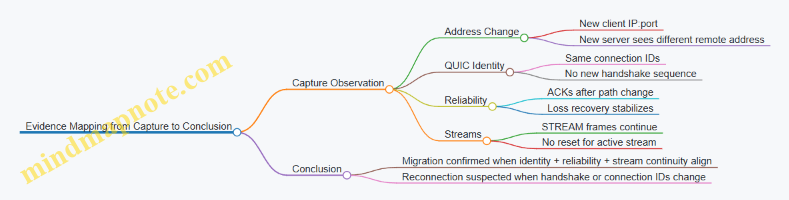
Practical Notes That Prevent False Positives
If you see address change but connection IDs differ, treat it as reconnection. If you see connection IDs match but the stream resets, treat it as migration followed by application-level failure or policy enforcement. If you see a handshake restart, treat it as a new connection even if the application appears to “resume.”
A clean run should produce a consistent story across layers: address changes in the network view, stable connection identity in QUIC, and uninterrupted stream behavior in HTTP/3.
11. Observability, Measurement, and Performance Engineering
11.1 Instrumentation Points for QUIC and HTTP3 Implementations
Good instrumentation answers three questions: what happened, when it happened, and why it happened. For QUIC and HTTP3, “why” usually means correlating transport events (loss, ACKs, congestion signals) with application events (streams, headers, responses). The trick is to instrument at the right layers and attach consistent identifiers so you can stitch timelines together.
Mind Map: Instrumentation Coverage
Connection Lifecycle Events
Instrument the start and end of the QUIC handshake with timestamps and outcomes. Record whether 0-RTT data was accepted, rejected, or ignored, because it changes what “early” application bytes mean. When the connection closes, log the close reason and whether it was local or peer-initiated. A practical example: if a client reports “first request timed out,” you can check whether the connection closed before the request stream was created.
Packet, ACK, and Loss Detection
Track packet send events with packet number ranges and the set of frames carried. When ACKs arrive, log the acknowledged packet ranges and the ACK delay value. Loss detection should emit a single event per detection decision, including the packet number range considered lost and the reason (e.g., time-based vs. threshold-based). Retransmission events should name which original frames were resent. This lets you answer: did the system retransmit because of real loss, or because of delayed ACKs?
Example: Suppose you see repeated retransmissions of STREAM frames on one stream while other streams progress. That pattern often indicates stream-level flow control or head-of-line behavior at the application layer, not a global congestion collapse.
Congestion Control and Pacing Signals
Instrument congestion window updates and pacing rate changes at the moment they affect sending. Also log ECN marks when observed and whether they were acted upon. If you estimate queueing delay, record it alongside the pacing decision. A useful sanity check is to compare “bytes sent per second” with “pacing rate” to confirm the sender is actually obeying its own pacing.
Flow Control and Backpressure
QUIC flow control failures are frequently the real reason for “slow responses.” Instrument both connection-level and stream-level flow control updates, plus counters for blocked states. Emit events when sending becomes blocked due to local limits and when the peer blocks you via advertised limits. For HTTP3, correlate these events with request/response stream activity.
Example: If response headers arrive quickly but the body stalls, you may see stream-level send blocked after headers, while the connection-level window still has room. That points to per-stream limits or application buffering strategy.
Stream and Frame Semantics
Log stream lifecycle transitions: created, started sending, first byte received, half-close, reset, and fully closed. For frames, record parsing errors and stream errors with the stream ID and error code. Keep byte counters per stream and per connection so you can compute effective throughput and identify “chatty” streams that send tiny frames.
Migration and Path Validation
When the network path changes, record the detected change, the new path characteristics you observe, and the outcome of address validation. Also log connection identifier changes so you can map packets to the correct logical path. If performance drops after roaming, you can check whether the sender waited for validation before resuming transmission.
HTTP3 Request and Response Instrumentation
Instrument HTTP3 at the request stream level. Record when request headers are decoded, when response headers are available, and when body chunks are delivered to the application. For errors, capture the HTTP3 stream error code and whether the QUIC stream reset preceded or followed the HTTP error.
QPACK Behavior Correlation
QPACK can cause stalls that look like transport issues. Instrument encoder insert events and decoder blocked/unblocked events. When the decoder blocks, log the reason (e.g., missing dynamic table entries) and the time until it unblocks. Then correlate that interval with QUIC ACK and loss events to see whether the stall is due to missing header references or delayed transport delivery.
Correlation Strategy with Identifiers
Use a consistent correlation key across layers: QUIC connection ID plus QUIC stream ID, and for HTTP3 also include the HTTP request/response stream role. Emit a single “timeline anchor” event when a request stream is created, then attach subsequent transport and HTTP events to that anchor.
Minimal Event Set for Fast Debugging
If you need a starting point, capture these events with timestamps: handshake outcome, connection close reason, packet sent ranges, ACK received ranges, loss detection decision, retransmission, flow-control blocked/unblocked, stream lifecycle transitions, HTTP header decode completion, and QPACK decoder blocked/unblocked.
Anchor: HTTP request stream created
Then: QUIC stream opened -> first bytes received
Transport: ACKs and loss decisions affecting those packets
HTTP: headers decoded -> body chunk delivery -> stream completion
This set is small enough to keep overhead reasonable, yet complete enough to explain most “it’s slow” reports without guessing.
11.2 Metrics for Throughput, Loss, Latency, and Stream Health
Good performance work starts with metrics that answer four questions: How much data moves? What goes missing? How long it takes? Whether streams behave like you expect. QUIC and HTTP/3 add structure—packets, acknowledgments, streams, and flow control—so the metrics should map to those structures rather than to vague “speed.”
Throughput Metrics That Actually Mean Something
Throughput is not one number. Track it at three layers:
- Application throughput: bytes delivered to the app per second, per request or per stream.
- Transport throughput: bytes acknowledged per second, which reflects what the network actually confirmed.
- Goodput: bytes that are useful at the application layer divided by time, excluding retransmitted payload.
A practical rule: if application throughput is high but transport throughput is low, you are likely buffering or stalled on flow control. If both are low, you are losing packets or constrained by congestion control.
Example: A video stream shows steady application bytes, but transport acknowledged bytes dip during bursts. That pattern often means the sender is pacing and the receiver is temporarily not advancing flow control windows.
Loss Metrics That Separate Loss from Delay
QUIC loss is best measured through acknowledgment behavior and recovery events, not just packet drops.
Track:
- Loss rate: lost packets per sent packets, based on packet number gaps and recovery decisions.
- Retransmission rate: retransmitted bytes per total bytes.
- Reordering depth: how far packets arrive out of order before being declared lost.
- Recovery time: time from first loss detection to the point when the missing data is acknowledged.
Example: If reordering depth is high but loss rate is low, you may be seeing path variability rather than true loss. If recovery time grows while loss rate stays constant, your loss detection or retransmission pacing may be too conservative for the workload.
Latency Metrics with Clear Ownership
Latency needs “ownership” so you can tell whether the delay is in the network, the protocol, or the application.
Use a small set of latency metrics:
- Handshake latency: time until keys are usable and the first HTTP/3 request can be sent.
- Time to First Byte: from request submission to first response data delivered.
- Per-stream RTT estimate: the sender’s view of round-trip time used for loss detection.
- Ack delay: how long the receiver waits before sending acknowledgments.
Example: Time to First Byte increases while handshake latency stays stable. That often points to stream scheduling, QPACK blocking, or flow control rather than connection setup.
Stream Health Metrics That Catch “It Works, But…”
Stream health metrics detect when streams are alive but not progressing.
Track:
- Stream completion rate: fraction of streams that finish within a target time.
- Stall duration: time between meaningful progress events on a stream.
- Reset rate: frequency of stream resets and the error codes involved.
- Flow control pressure: how often the sender hits stream-level or connection-level flow control limits.
- QPACK blocking indicators: how often header decoding waits for required dynamic table entries.
Example: A request stream completes, but it repeatedly stalls for short intervals. If stalls correlate with flow control pressure, you can reduce concurrency or adjust pacing. If stalls correlate with header decoding waits, you can change header patterns to reduce dynamic table churn.
Mind Map: Metrics and What They Diagnose
Correlating Metrics into Diagnoses
Metrics become useful when you correlate them with protocol events.
- Throughput drop + loss increase: congestion control and loss recovery are dominating.
- Throughput drop + loss stable + ack delay increase: receiver acknowledgment behavior or scheduling is slowing progress.
- Latency increase + resets increase: stream-level errors or header decoding issues may be causing early termination.
- Stalls + flow control pressure: sender is waiting for window updates; reduce concurrent streams or adjust pacing.
Example: During a test, you observe stable loss rate but rising Time to First Byte and increasing stall duration. If ack delay also rises, the receiver is acknowledging less frequently, which can delay retransmission triggers and stream progress.
Minimal Metric Collection Checklist
Collect metrics that let you compute the four core questions without guesswork:
- Bytes sent, bytes acknowledged, bytes delivered to app.
- Packet loss decisions, retransmissions, and recovery times.
- Handshake completion time, Time to First Byte, RTT estimate, ack delay.
- Stream progress events, stalls, resets, and flow control pressure.
If you can plot these on the same timeline, you can usually explain performance changes with one or two causal links. QUIC is deterministic enough that the metrics should point to a specific mechanism, not just a general “network is bad.”
11.3 Interpreting Traces With Wireshark and Key Log Files
When you inspect QUIC and HTTP/3 traffic, you’re really answering two questions: what happened on the wire, and why it happened. Wireshark tells you what bytes arrived and when; key log files help you interpret those bytes as meaningful protocol events, such as handshake progress, stream frames, and header decoding.
Trace Foundations You Should Get Right First
Start with a clean capture and a consistent filter strategy. Confirm you’re seeing UDP packets for the correct 5-tuple, and that the capture includes both directions. QUIC is packet-numbered per connection, so missing packets can make loss recovery look “mysterious” when it’s simply incomplete observation.
Then establish your timeline. In Wireshark, use packet ordering and timestamps to correlate: handshake packets first, then application data, then any retransmissions or stream resets. If you see application frames before the handshake completes, you’re likely looking at 0-RTT or a partial capture.
Wireshark Views That Map to QUIC Reality
Wireshark’s QUIC dissection is most useful when you read it in layers:
- Transport layer: packet number, packet type, ACK ranges, and loss-related behavior.
- Crypto layer: handshake messages and key updates.
- Stream layer: stream IDs, offsets, and frame types.
- HTTP/3 layer: request/response semantics and QPACK-related behavior.
A practical habit: when something looks wrong, jump to the packet details and check whether Wireshark is treating it as Initial, Handshake, or 1-RTT. Many “bugs” are actually misclassification caused by missing decryption keys or incomplete key log configuration.
Key Log Files for Meaningful Decryption
Key log files let Wireshark decrypt QUIC so it can show frames and headers instead of raw payload. The key idea is that QUIC derives traffic keys from secrets negotiated during the TLS 1.3 handshake. If the key log file is missing, mismatched, or generated with different process parameters, Wireshark will fall back to undeciphered payload.
Use a deterministic workflow:
- Generate the key log file from the same client or server process that produced the capture.
- Ensure the key log file is available to Wireshark before opening the capture.
- Verify decryption by checking that Wireshark shows decrypted QUIC packet contents and HTTP/3 frames.
If decryption fails, don’t guess. Confirm that the key log file contains entries for the connection you captured, and confirm that the capture includes the handshake packets that establish those secrets.
Mind Map: For Trace Interpretation
Systematic Workflow for a Single Connection
- Identify the connection: pick a packet that clearly belongs to the QUIC flow and note the connection identifiers shown by Wireshark.
- Locate the handshake boundary: find the transition from Initial/Handshake to 1-RTT. This is where application data becomes expected.
- Check ACK behavior: look for ACK frames and whether retransmissions occur. If you see retransmissions without corresponding ACKs, suspect packet loss or capture gaps.
- Inspect stream frames: for each stream, verify ordering and offsets. QUIC allows out-of-order delivery, so “out of order” in time doesn’t automatically mean “out of order” in stream offsets.
- Interpret HTTP/3 semantics: confirm that request headers arrive before response headers on the expected streams, and watch for stream resets that explain abrupt termination.
Example: Diagnosing a QPACK Blocking Symptom
Suppose you see response body data arriving, but response headers appear incomplete or delayed in Wireshark. With decryption enabled, check for QPACK-related behavior:
- Look for decoder instructions that depend on dynamic table entries.
- Identify whether the decoder is waiting for insert acknowledgments.
- Correlate the timing: header decoding should unblock once the required dynamic table entries are available.
A concrete check: compare the timestamps of QPACK insert-related events with the timestamps of the HTTP/3 header blocks. If inserts arrive later than expected, you may be observing normal behavior under loss or reordering, not a protocol violation.
Example: Verifying Loss Recovery with ACK Ranges
If a stream stalls, inspect the QUIC transport details for ACK ranges. You want to see:
- Which packet numbers were acknowledged.
- Whether missing packet numbers trigger retransmission.
- Whether retransmitted packets carry the expected stream offsets.
When retransmissions occur, Wireshark should show the same stream data being resent with the correct offsets. If offsets don’t match, you’re likely looking at different streams or a different connection identifier.
Common Failure Modes and How to Spot Them Quickly
- Undecrypted payload: key log mismatch or missing handshake secrets.
- Wrong packet type: incomplete capture or decryption not applied.
- Misleading “loss”: capture gaps that omit ACKs or retransmissions.
- Confusing stream order: time order differs from stream offset order.
A good trace is boring: clear handshake boundary, consistent ACKs, and stream frames that line up with offsets. When it’s not boring, the protocol still gives you the clues—you just have to read them in the right layer order.
11.4 Building Reproducible Test Scenarios with Network Emulation
Reproducible tests start with a simple rule: the network is part of the test, not a background condition. If you can’t describe the emulation settings in a way another engineer can re-run, you’re measuring your own uncertainty.
Define the Test Goal and Measurable Outcomes
Begin by writing one sentence that states what you want to prove. Examples:
- “Under 2% random loss and 80 ms RTT, interactive requests should complete within 95th percentile latency bounds.”
- “With path migration enabled, the connection should continue without a full handshake.”
Then list the metrics you will record. For QUIC and HTTP/3, keep it concrete:
- Handshake completion time and whether 0-RTT was accepted.
- Loss recovery behavior: time to first retransmission and number of recovery events.
- Stream-level effects: queueing delay, flow-control stalls, and stream reset counts.
- Application-visible timing: request start to response first byte.
Choose a Scenario Template and Lock It Down
A scenario template is a fixed set of emulation parameters plus a fixed traffic pattern. Lock these inputs before you tune anything.
Traffic pattern examples
- Single stream request/response at a fixed interval.
- Many concurrent streams with a mix of small and large payloads.
- Bursty traffic with a defined idle gap to test timeouts and keepalive behavior.
Emulation parameter examples
- RTT distribution (constant vs jittered).
- Packet loss model (random vs bursty).
- Reordering rate and maximum reordering depth.
- Bandwidth cap and queue size.
Keep the traffic generator deterministic: fixed seeds for request timing, fixed payload sizes, and stable concurrency limits.
Build a Mind Map of What Must Be Controlled
Mind Map: Reproducible Network Emulation for QUIC and HTTP/3
Create a Scenario Manifest and Use It Every Time
A scenario manifest is a plain-text checklist you attach to every run. It prevents “works on my machine” from becoming a lifestyle.
Include:
- Emulation settings: RTT, jitter, loss, reordering, bandwidth, queue.
- Traffic generator settings: request rate, concurrency, payload sizes, duration, random seed.
- QUIC/HTTP/3 configuration: stream limits, idle timeout, congestion control choice, QPACK behavior.
- Environment details: CPU pinning if relevant, container limits, and clock synchronization method.
Validate Reproducibility Before You Trust Results
Run the same scenario multiple times and measure variance. A practical approach:
- Do 5 runs for a quick check.
- Compare median and 95th percentile latency, plus counts of retransmissions and stream resets.
- If variance is high, fix determinism first (seeds, timing sources, concurrency scheduling) before changing network parameters.
Example Scenario: Long RTT with Loss and Reordering
Goal: confirm that loss recovery and stream scheduling behave consistently under long RTT.
Scenario
- RTT: 120 ms constant with 10 ms jitter.
- Loss: 1% random loss plus 0.5% burst loss lasting 2–3 packets.
- Reordering: 0.2% packets with a small reordering depth.
- Bandwidth: 20 Mbps with a queue sized to hold about 200 ms of data.
Traffic
- 20 concurrent streams.
- 10 small requests (1–4 KB) and 10 medium requests (64–128 KB) per batch.
- Batch interval: 1 second, total duration: 60 seconds.
- Fixed seed for request start times.
Pass criteria
- Handshake success rate is stable across runs.
- Retransmission counts vary within a narrow band.
- No unexpected surge in stream resets.
- HTTP/3 response first byte timing shows consistent tail behavior.
Example: Trace Alignment Rules for Debugging
When you compare runs, align on events rather than wall-clock time. For instance:
- Use the client’s “handshake complete” timestamp as t=0.
- Measure request completion relative to that anchor.
- For loss recovery, record the first packet number marked lost and the time until the first retransmission is observed.
This turns “the traces look different” into “the recovery started 35 ms later in run 3,” which is the kind of difference you can act on.
Reporting the Results Without Hand-Waving
Summarize each scenario with:
- A manifest snapshot.
- Metric table: median and 95th percentile latency, retransmission counts, stream reset counts.
- A short narrative that ties observed behavior to controlled inputs, such as “tail latency increases when loss bursts coincide with QPACK decoding stalls.”
If you can’t explain a result using only the manifest and the traces, the scenario isn’t yet reproducible in the way that matters.
11.5 Practical Example: Creating a Performance Regression Checklist
A performance regression checklist is a disciplined way to answer one question: “Did we make things worse, and where?” For QUIC and HTTP/3, the checklist should cover transport behavior, HTTP/3 framing, and the measurement method itself. The goal is not to chase a single number, but to catch specific failure modes like slower loss recovery, QPACK stalls, or changed stream scheduling.
Step 1: Define the Baseline and the Scope
Start by freezing the variables that can change without code changes: test topology, client/server versions, OS settings, and network emulation profile. Pick one baseline build and one baseline configuration. Then define what “regression” means for your workload: latency to first byte, time to complete N requests, sustained throughput, and stability under loss.
Example scope for a mixed workload:
- 10 concurrent HTTP/3 requests per connection
- 1 connection per client process
- Payload sizes: 1 KB headers-heavy, 64 KB body, and 1 MB streaming
- Network profiles: clean, 2% loss, 100 ms RTT with jitter, and a reordering profile
Step 2: Instrument What You Will Blame
If you cannot observe it, you cannot fix it. Your checklist should require these measurements for every run:
- QUIC loss and recovery events: packet loss rate, time-to-retransmit, and ack delay behavior
- Congestion control signals: cwnd evolution and pacing changes
- Stream-level flow control: blocked-by-connection-window vs blocked-by-stream-window
- HTTP/3 framing: request/response ordering, stream resets, and error codes
- QPACK behavior: encoder insert/ack counts and decoder blocking duration
A simple rule: every metric should map to a hypothesis. If a metric cannot explain a symptom, it probably does not belong in the checklist.
Step 3: Create a Run Matrix That Catches Common Regressions
Use a small but targeted matrix. Too many combinations create noise; too few miss real issues.
Example run matrix:
- Network: clean, 2% loss, 100 ms RTT + 10 ms jitter, 100 ms RTT + reordering
- Workload: headers-heavy (many small responses), mixed (small + medium), streaming (large body)
- Concurrency: 1, 10, 50 concurrent requests per connection
For each cell, record at least:
- p50 and p95 time-to-first-byte
- completion time for the workload
- retransmission count and recovery duration
- QPACK decoder blocking time
- number of stream resets
Step 4: Add Pass/Fail Thresholds with Reasonable Tolerance
Thresholds should reflect measurement variance. A practical approach is to use relative change from baseline plus an absolute floor.
Example thresholds:
- p95 time-to-first-byte: fail if +10% or +20 ms, whichever is larger
- completion time: fail if +15%
- retransmission count: fail if +25% under the same loss profile
- QPACK decoder blocking time: fail if it increases by any amount that exceeds 5 ms median
- stream resets: fail if any new non-zero count appears
When a threshold fails, the checklist should force a classification: transport regression, HTTP/3 regression, QPACK regression, or measurement regression.
Step 5: Use a Mind Map to Keep the Checklist Coherent
Performance Regression Checklist Mind Map
Step 6: Provide a Concrete Triage Workflow
When a run fails, do not start by rewriting code. Follow a deterministic path.
- Symptom first: If p95 time-to-first-byte rises but throughput stays similar, suspect handshake timing, QPACK blocking, or stream scheduling.
- Transport check: If retransmissions increase and recovery duration grows, inspect loss detection and ack delay behavior.
- HTTP/3 framing check: If stream resets appear or response ordering changes, inspect error handling paths and stream lifecycle.
- QPACK check: If decoder blocking time increases, compare insert/ack counts and ensure encoder/decoder streams are progressing.
- Measurement drift check: If only one network profile fails, verify CPU load, timer resolution, and emulation parameters.
Step 7: Example Checklist Entry You Can Copy
Test case: Headers-heavy workload, 10 concurrent requests per connection, 100 ms RTT + 10 ms jitter.
- Record
- p50/p95 time-to-first-byte
- retransmission count and recovery duration
- QPACK decoder blocking median and p95
- stream resets count
- Thresholds
- p95 TTFB: fail if +10% or +20 ms
- QPACK blocking: fail if median increases by >5 ms
- stream resets: fail if any new resets appear
- Triage mapping
- If QPACK blocking fails: inspect QPACK insert/ack progression and decoder blocking intervals
- If retransmission fails: inspect loss recovery timeline and ack delay
- If resets fail: inspect stream reset reasons and timing relative to request start
This structure keeps the checklist systematic: it starts with controlled baselines, then enforces observability, then evaluates with thresholds, and finally routes failures to the right subsystem using trace-backed evidence.
12. Implementation Guidance and Interoperability Testing
12.1 Server and Client Configuration Patterns for Common Deployments
A solid QUIC/HTTP3 deployment starts with predictable defaults and a small set of knobs you can reason about. The goal is not to “tune everything,” but to make behavior stable under real network conditions: loss, reordering, NAT rebinding, and varying RTT.
Mind Map: Server and Client Configuration Patterns
Server Configuration Patterns
1) Bind predictably and keep UDP handling boring. Bind a UDP socket on the intended interface(s) and ensure the server can handle bursts without blocking the receive path. If you run multiple instances behind a load balancer, confirm that the QUIC traffic stays on the same instance for the lifetime of a connection, or that your load balancer supports QUIC-aware routing.
2) Choose a Connection ID strategy that matches your routing reality. Connection IDs let a connection survive address changes, but they also affect how much state you keep and how you correlate logs. Use a Connection ID length and rotation policy that your deployment can track in observability. If you rotate aggressively, ensure your server can still map incoming packets to the right connection quickly.
3) Set transport parameters to protect the server while preserving client usability. Limits like maximum streams and flow control windows should reflect your expected concurrency and payload sizes. A common mistake is setting very small stream limits, which forces clients into extra round trips for new streams. Another mistake is setting huge limits without capacity planning, which can amplify memory pressure when many clients connect.
4) Pick idle timeout and keepalive behavior intentionally. Idle timeout controls when the server frees connection state. For interactive workloads, too-short timeouts cause frequent handshakes; too-long timeouts can waste resources. If you expect NATs to drop mappings, keepalive behavior should be consistent with your idle timeout so the connection stays alive long enough to be useful.
5) Configure QPACK behavior to avoid decoder stalls. QPACK is where header compression meets flow control. Ensure your server’s QPACK settings align with your expected header sizes and request rates. If you see stalls, it’s often because the decoder can’t progress due to missing dynamic table entries, not because the network is “slow.”
Client Configuration Patterns
1) Reuse connections when it helps, and close them when it doesn’t. For HTTP/3, connection reuse reduces handshake overhead and improves latency consistency. However, if your client talks to many hosts or uses short-lived sessions, reuse can increase resource usage. A practical pattern is to reuse per origin and cap the number of concurrent connections per host.
2) Decide on 0-RTT policy based on request safety. 0-RTT can reduce latency, but it must not cause unintended side effects. A safe deployment pattern is: allow 0-RTT only for idempotent requests (like GET) and disable it for requests that change server state unless you have explicit replay protections at the application layer.
3) Set timeouts that match QUIC’s recovery behavior. QUIC loss recovery is not identical to TCP’s retransmission timing. If your client times out too aggressively, you’ll abort connections that would have recovered. If it times out too slowly, you’ll keep dead connections around. Use measured RTT distributions from your environment to choose conservative initial timeouts.
4) Manage concurrency with backpressure, not hope. HTTP/3 allows multiple streams over one connection, but the connection still has flow control limits. Implement a strategy that limits in-flight work per connection and reacts to backpressure by pausing request generation rather than buffering unbounded data.
Example: A Common Web Service Deployment
A typical setup for a web service looks like this:
- Server: one UDP listener per instance, stable Connection ID mapping for logging, transport parameters sized for expected concurrency, and an idle timeout tuned to NAT behavior.
- Client: per-origin connection reuse, 0-RTT enabled only for GET, concurrency capped to avoid flow control pressure, and timeouts derived from observed RTT.
Here’s a compact checklist you can apply during rollout:
| Area | Server Pattern | Client Pattern | Validation Signal |
|---|---|---|---|
| Limits | Set max streams and flow control to match capacity | Cap concurrent streams | Fewer stream creation stalls |
| Timeouts | Idle timeout aligned with NAT mapping | Recovery-aware request timeouts | Reduced premature aborts |
| Headers | QPACK settings consistent with header rate | Handle decoder progress | No repeated header stalls |
| Security | TLS 1.3 correct cert chain | 0-RTT only for safe methods | No replay-sensitive failures |
Example: Debugging a Misconfiguration Without Guessing
If clients report intermittent slow responses, start by checking whether the issue is transport recovery or application scheduling.
- Confirm handshake completion timing and whether 0-RTT is used.
- Inspect loss recovery events and ACK delays to see if the connection is struggling.
- Check for QPACK-related stalls that can delay request processing even when the network is fine.
- Verify stream concurrency and flow control: if the client sends too many concurrent streams, it may hit backpressure and appear “slow.”
When you fix one knob, re-run the same scenario and compare the trace markers. QUIC behavior is deterministic enough that you can usually pinpoint the cause without turning every parameter into a mystery.
12.2 Interoperability Pitfalls with HTTP3 and QPACK Settings
Interoperability issues in HTTP/3 usually show up as “it works on my machine” symptoms: requests stall, headers arrive late, or streams reset in ways that look unrelated to the actual bug. Most of those failures trace back to mismatched expectations between peers about QPACK behavior, limits, and how endpoints react to blocking.
Core Interoperability Model
HTTP/3 carries requests and responses on QUIC streams, but header compression is handled by QPACK. QPACK splits responsibilities:
- The encoder sends compressed header blocks on the request/response stream.
- The decoder may need dynamic table entries that arrive on dedicated control streams.
- If the decoder references entries it has not received yet, it can block until they arrive or until the endpoint decides to abort.
Interoperability pitfalls happen when one side assumes a different QPACK mode, uses different limits, or treats blocking differently.
Mind Map: Interoperability Failure Points
QPACK Settings That Commonly Break Compatibility
Dynamic Table Capacity
If the encoder’s dynamic table capacity is larger than the decoder’s, the decoder may reject inserts or fail to keep up with references. The practical symptom is that header blocks decode slowly or trigger stream resets.
Example: A client uses a larger dynamic table and compresses headers by referencing many dynamic entries. A server configured with a smaller capacity may not accept the insert stream at the expected rate, so the decoder cannot resolve references quickly.
Mitigation: Ensure both endpoints agree on QPACK dynamic table capacity through transport parameters and that your implementation enforces the negotiated limits rather than local defaults.
Maximum Blocked Streams
QPACK defines a limit on how many streams the decoder can keep blocked waiting for dynamic entries. If one endpoint sets this too low, it may abort streams that another endpoint would tolerate.
Example: A CDN edge server sets a low maximum blocked streams value to reduce memory usage. A mobile client sends many concurrent requests whose header blocks reference dynamic entries not yet available. The server hits the blocked limit and resets streams, even though the missing entries would have arrived moments later.
Mitigation: Choose a maximum blocked streams value that matches expected concurrency and loss conditions, and test with bursty request patterns.
Encoder Stream and Acknowledgment Behavior
QPACK uses acknowledgments to let the encoder know which inserts the decoder has processed. If an implementation delays acknowledgments or mishandles them, the encoder can overrun the decoder’s ability to track dynamic entries.
Example: A client buffers acknowledgments until it sees certain frames, but the server expects timely acknowledgments to manage its insert rate. Under packet loss, the buffering delays compound, and the encoder’s control traffic becomes inconsistent with the decoder’s state.
Mitigation: Treat acknowledgments as state-critical. Drive them from decoder progress, not from application-level events.
Ordering and Loss: When “It’s Just Headers” Isn’t
Control streams and header blocks share the same QUIC transport, so loss and congestion affect them together. A subtle interoperability issue occurs when one endpoint assumes that control traffic will arrive early enough to avoid blocking, while the other endpoint is strict about blocked states.
Example: Under constrained networks, inserts on the QPACK control stream arrive late. One endpoint tolerates blocking longer and continues decoding once inserts arrive. The other endpoint enforces a shorter blocked timeout and resets the affected request stream.
Mitigation: Ensure your blocked-timeout and reset logic aligns with the negotiated QPACK behavior and that you test under loss and reordering, not just latency.
Stream Reset Semantics and Error Mapping
When QPACK decoding fails, endpoints must map that failure to QUIC stream errors and HTTP/3 error handling consistently. Interoperability bugs often come from treating a QPACK decoding failure as a generic application error, which can cause the peer to retry or to keep sending on streams that should be terminated.
Example: A server treats a QPACK decode failure as a recoverable header issue and continues the response stream. A client interprets the missing headers as a fatal decode error and resets the stream, leading to confusing partial behavior.
Mitigation: On decode failure, terminate the affected stream in a way that matches the peer’s expectations: consistent error codes, consistent reset timing, and no continued emission on a stream that cannot be decoded.
Practical Checklist for Interoperability Testing
- Verify negotiated QPACK parameters at connection setup and ensure they override local defaults.
- Test concurrent bursts that force dynamic table references before inserts arrive.
- Introduce controlled loss so control streams and header blocks desynchronize.
- Confirm blocked-stream limits are not exceeded under your target concurrency.
- Validate error mapping by checking that both sides reset the same stream types under the same failure conditions.
Example: Minimal Interop Debug Scenario
A client sends 50 concurrent requests with compressed headers that reference dynamic entries. The server has a low maximum blocked streams value. Under mild loss, inserts arrive late. The server blocks decoding for some streams, hits the blocked limit, and resets those streams. The client then observes request failures that look like application issues.
The fix is not “increase timeouts blindly.” It is to align QPACK settings and ensure the encoder’s insert/ack pacing matches the decoder’s capacity and blocked limits, then re-test with the same concurrency and loss profile.
12.3 Validating Stream and Frame Semantics Under Stress Conditions
Validating stream and frame semantics means proving that your implementation behaves correctly when the network misbehaves: reordering, loss, bursts, and timing shifts. The goal is not just “it works,” but “it works for the right reasons,” even when the trace looks messy.
Core Semantics to Validate
Start with a checklist that maps directly to observable behavior.
- Stream lifecycle correctness: creation, data transfer, end-of-stream signaling, reset behavior, and cleanup. Under stress, you must ensure that state transitions are monotonic and that no late frames resurrect closed streams.
- Frame parsing correctness: every frame type must be parsed deterministically, with strict length checks and correct handling of unknown or invalid fields.
- Ordering rules within a stream: QUIC preserves byte order per stream; HTTP/3 preserves frame order within the request/response stream. If you see reordering at the application layer, it’s usually buffering logic, not transport.
- Flow control interactions: flow control limits must gate sending and receiving without deadlocking. Stress often reveals “almost correct” backpressure handling.
- Error semantics: stream errors, connection errors, and how you surface them to the application. A reset should terminate only what it claims to terminate.
Stress Scenarios That Expose Bugs
Use scenarios that target specific failure modes.
- Loss bursts during header-heavy traffic: forces retransmission and tests whether HTTP/3 frame boundaries and QPACK-related behavior remain consistent.
- Reordering across packets: validates that your parser and stream assembler handle out-of-order arrival without mixing bytes from different offsets.
- Concurrent streams with mixed sizes: stresses scheduling and ensures that one large stream does not starve small control frames.
- Frequent resets: tests that reset frames stop further delivery and that your application does not read stale buffers.
- Backpressure pressure: artificially low flow control windows to confirm that you pause sending at the right layer.
Mind Map: Validation Plan
A Systematic Test Method
Treat validation as a pipeline: generate, observe, assert.
- Generate deterministic traffic: create a workload that produces known stream IDs and known frame sequences. For example, send three request streams concurrently: one with small headers, one with large headers, and one that triggers a reset mid-body.
- Instrument at three layers: (a) transport-level stream assembly events, (b) HTTP/3 frame decode events, and (c) application callbacks. The timestamps don’t need to match perfectly; the ordering of events must.
- Assert invariants at boundaries:
- After a stream reset, assert that no further frame decode occurs for that stream.
- When an end-of-stream is signaled, assert that the application receives exactly one completion event.
- During loss and retransmission, assert that frame boundaries remain stable; you should not “re-split” a frame differently after recovery.
- Cross-check with traces: when an assertion fails, correlate the failing event with packet-level offsets. Most semantic bugs reduce to one of two issues: incorrect offset-to-buffer mapping, or incorrect state transition on receiving end/reset.
Example: Reset Semantics Under Loss
Setup: Send a request stream that begins with a headers frame, then sends body data in two chunks. Force a loss burst so the second chunk’s packets are delayed. Midway, trigger a stream reset from the sender.
Expected behavior:
- The receiver may have already decoded the first body chunk.
- After the reset is processed, the receiver must not deliver the delayed second chunk to the application.
- The receiver should not emit a second completion event.
What to assert:
- Frame decode log shows headers and first body chunk.
- After reset, frame decode for that stream stops.
- Application sees one completion or one error, not both.
Example: Frame Boundary Integrity with Reordering
Setup: Create a stream containing a sequence of frames whose serialized lengths are distinct. Emulate packet reordering so that later bytes arrive first.
Expected behavior:
- The stream assembler reconstructs the byte stream correctly.
- The frame decoder emits frames in the correct order and with correct lengths.
What to assert:
- The decoder never reports “frame length exceeds available bytes” for valid traffic.
- The emitted frame sequence matches the generator’s sequence exactly.
Practical Assertion Patterns
Keep assertions tight and local.
- State monotonicity: record stream state transitions and assert they never go backward.
- Delivery uniqueness: each logical completion callback fires once per stream.
- Reset scoping: a reset for stream X never affects stream Y.
- Decode determinism: given the same assembled byte sequence, frame decode results are identical.
Failure Triage Without Guesswork
When something fails, classify it quickly.
- If frame boundaries shift after recovery, focus on offset-to-assembly mapping.
- If the application receives data after reset, focus on state gating in the delivery path.
- If you see deadlocks under backpressure, focus on where you block: sending, decoding, or callback dispatch.
A good stress validation run ends with a small set of precise, reproducible failures. That’s the point: semantics should be testable, not just believable.
12.4 Security Validation for Handshake and Keying Behavior
Security validation for QUIC and HTTP/3 is mostly about proving that both sides agree on keys, that those keys are used only for the intended cryptographic context, and that failures are handled in ways that don’t leak useful information. The goal is not just “it connects,” but “it connects for the right reasons,” even when packets are lost, reordered, or replayed.
Handshake Message Flow and State Checks
Start by validating the handshake as a state machine. For a full handshake, the server and client must complete the TLS 1.3 exchange, then derive QUIC secrets, then confirm that encrypted handshake traffic is actually decryptable with the derived keys.
A practical validation checklist:
- Confirm that the client does not accept application data keys before the handshake keys are established.
- Confirm that the server does not accept client application data until it has derived the same secrets.
- Verify that handshake completion triggers the expected transition in your connection object, including stream handling rules.
Easy example: log the derived secret labels (not the secret bytes) at each stage. If your implementation prints “handshake traffic keys ready” on the client but never on the server, you likely have a mismatch in transport parameters or TLS transcript handling.
TLS 1.3 Transcript Integrity and QUIC Secret Derivation
QUIC uses TLS 1.3, but the transcript is bound to QUIC-specific inputs such as connection identifiers and transport parameters. Validation should therefore include:
- Ensuring the TLS transcript bytes used for key schedule match what the QUIC layer claims it used.
- Ensuring transport parameters are parsed before key derivation and that negotiation failures abort cleanly.
Easy example: create a test where the client sends a transport parameter that the server rejects. Your server should fail the handshake before deriving application traffic keys, and your client should treat the failure as non-recoverable for that connection attempt.
0-RTT and Replay Safety Validation
0-RTT is where “works on my network” becomes “works on my attacker’s network.” Validation must ensure:
- The server’s policy for accepting 0-RTT is enforced consistently.
- Application data sent in 0-RTT is either replay-safe by design or gated behind logic that prevents unsafe side effects.
Easy example: implement a request that increments a counter. Send it as 0-RTT. In tests, simulate a replay by reusing the same early data. The server must either reject the replay or ensure the operation is idempotent (for example, using a client-provided request identifier stored for deduplication).
Key Update and Key Separation Rules
After handshake, QUIC may update keys. Validation should confirm:
- Key updates use the correct epoch and do not reuse keys across encryption contexts.
- Packet protection keys and header protection keys are derived and applied consistently.
Easy example: force a key update after a small number of packets in a test environment. Then verify that decrypting with the old keys fails for packets after the update, while decrypting with the new keys succeeds.
Connection Migration and Keying Consistency
Migration changes the network path but should not change cryptographic identity. Validation should confirm that:
- Connection identifiers map to the correct cryptographic context.
- Address changes do not cause the implementation to “reset” keys or accept packets under the wrong context.
Easy example: migrate mid-transfer by switching the client’s source IP in a controlled test. The connection should continue decrypting packets without re-handshaking, and rejected packets should fail authentication rather than being silently ignored.
Failure Handling Without Useful Leakage
When validation fails, the system should avoid giving an attacker a detailed oracle. That means:
- Use consistent error handling paths for decryption failures versus authentication failures.
- Ensure that logs used in production do not include sensitive material or overly specific reasons.
Easy example: in a test harness, intentionally corrupt a single byte in the encrypted payload. Your server should terminate the connection (or stream) deterministically, and your client should not be able to distinguish “wrong key” from “wrong packet number” based on observable behavior.
Mind Map: Security Validation Flow
Example: Minimal Validation Test Plan
Run a small suite that covers the cryptographic lifecycle:
- Full handshake success with negotiated transport parameters.
- Rejected transport parameter causes early abort before application keys.
- 0-RTT request is replayed and either rejected or deduplicated.
- Key update occurs and old keys no longer decrypt new packets.
- Migration changes path and decryption continues under the same keys.
- Corrupted ciphertext triggers deterministic failure without revealing sensitive distinctions.
If these tests pass, you’ve validated the handshake and keying behavior in the ways that matter: agreement on secrets, correct use of those secrets, and safe handling of failure modes.
12.5 Practical Example: Test Plan for Production Readiness
A production-ready QUIC and HTTP3 setup is less about passing a single “works on my machine” test and more about proving that behavior stays correct when the network misbehaves. This plan is written for a server and one or more clients, but the same structure applies to load tests and canary deployments.
Test Scope and Success Criteria
Start by listing what “ready” means in measurable terms.
- Correctness: requests complete with expected status codes and bodies; header decoding never deadlocks; stream resets map to the right HTTP semantics.
- Transport health: handshake succeeds under normal and lossy conditions; loss recovery completes; congestion control does not stall streams indefinitely.
- Performance stability: latency and throughput remain within agreed bounds across repeated runs.
- Operational safety: logs are actionable; metrics show clear failure modes; resource usage stays bounded.
Mind Map: Production Readiness Test Flow
Test Matrix That Actually Covers Failure Modes
Use a small set of network profiles that target known pain points.
- Normal: baseline RTT, low loss, stable bandwidth.
- Loss and Jitter: moderate RTT with controlled packet loss and variable delay.
- High Latency: long RTT with delayed ACK behavior.
- Reordering: out-of-order delivery without extreme loss.
- Bandwidth Variability: periodic throttling to force flow control pressure.
For each profile, vary:
- Concurrency: e.g., 10, 100, 500 concurrent requests.
- Stream mix: short request/response pairs plus one longer response stream.
- Header sizes: small headers and larger sets that stress QPACK.
Step-by-Step Execution
Handshake and Security Validation
Run a handshake suite that checks both success and failure clarity.
- Confirm that TLS 1.3 keys are established and that application data does not appear before handshake completion.
- Attempt session resumption and verify that 0-RTT behavior does not cause incorrect request replay handling.
- Intentionally misconfigure one client parameter (like transport limits) to ensure the server rejects cleanly.
Stream, Loss Recovery, and Flow Control
For each network profile:
- Send a workload that forces loss recovery by using a payload size that spans multiple QUIC packets.
- Verify that retransmissions complete and that the application receives ordered HTTP3 semantics even when transport delivery is not ordered.
- Apply backpressure by limiting server-side processing so flow control limits are exercised; ensure streams do not hang.
HTTP3 Frame and QPACK Behavior
This is where many “mostly works” systems fail.
- Use a request set that triggers QPACK dynamic table usage, then confirm that decoding completes without blocking indefinitely.
- Include a scenario with stream resets mid-response and verify that the client surfaces the correct failure for that request.
- Confirm that header encoding and decoding remain consistent across repeated runs.
Connection Migration and Resilience
If your environment expects address changes, test it explicitly.
- Simulate a client IP/port change while keeping the same logical session.
- Verify that the server accepts the new path using connection identifiers and that in-flight streams either complete or fail deterministically.
Trace-Based Validation Checklist
For each run, collect traces and check these invariants.
- Handshake timeline: no application frames before keys are ready.
- Loss recovery: ACKs advance packet numbers; retransmissions occur when expected.
- Flow control: send windows shrink and expand without deadlock.
- QPACK: encoder/decoder synchronization progresses; no indefinite waiting.
- HTTP3 mapping: stream resets correspond to the right request stream.
Example: Concrete Test Run Template
Test Run: High Latency With Loss
- Network: RTT 200ms, loss 2%, jitter 10ms, bandwidth 20Mbps
- Clients: 50 concurrent
- Workload: 40% short responses, 60% medium responses
- Headers: 10 fields average, plus 1% requests with 80 fields
- Steps
- Warm-up 30s
- Execute 5 minutes of steady load
- Pause 10s and resume for 2 minutes
- Trigger 10 connection migrations during steady load
- Pass Criteria
- 99.9% requests complete
- No client-side deadlocks
- P95 latency within agreed bound
- No unbounded memory growth
Gate Release with Clear Thresholds
Release only when repeated runs agree.
- Require at least three runs per network profile.
- Set thresholds for error rate, latency percentiles, and resource ceilings.
- Define rollback triggers based on correctness failures first, then performance regressions.
Operational Review That Completes the Picture
After tests, review logs and metrics together.
- Confirm that failures include enough context to identify whether the issue is handshake, QPACK, stream reset, or flow control.
- Ensure metrics show distinct counters for transport-level events and HTTP-level outcomes.
This plan turns production readiness into a checklist of observable behaviors. If the system stays correct under the targeted network profiles and the traces show progress rather than waiting, you can be confident the setup is not just functional, but dependable.