Miniaturized Harmonic Drives and Precision Servos
1. Scope and Design Goals for Miniaturized Actuation
1.1 Define Component Targets for Drone and Robotics Use Cases
Component targets turn a “we need precision” wish into measurable requirements. For miniaturized harmonic drives and precision servos, the targets should be set in a chain: mission needs → motion requirements → load and environment → geometry and materials → manufacturing and verification. If you skip a link, you’ll end up tuning the wrong thing.
Start with the Use Case Motion Profile
Begin by writing down what the actuator must do, not what it should feel like. For a drone, that might be gimbal pointing or control-surface actuation; for a robot, it might be joint positioning or link actuation.
Define these motion quantities:
- Range of motion: total angle or linear travel.
- Resolution: smallest meaningful step at the output.
- Speed: maximum angular velocity and typical operating speed.
- Acceleration: peak acceleration during starts and stops.
- Duty cycle: how long it runs at load before cooling.
Example: A compact gimbal needs ±45° output, smooth tracking at 30°/s, and the ability to correct small disturbances. If the output resolution target is 0.01°, you can back-calculate the required encoder resolution and gear reduction.
Convert Motion into Output Torque and Stiffness
Next, translate motion into forces. Harmonic drives are often chosen for their reduction and low backlash, but they still must carry torque without excessive deflection.
Set targets for:
- Peak output torque under worst-case load.
- Continuous output torque for thermal stability.
- Output torsional stiffness to limit pointing error under load.
- Allowable backlash at the output for control stability.
Example: If a robot joint must hold a 0.5 N·m gravitational load with a maximum pointing error of 0.05°, you can estimate the required stiffness and then check whether the gear mesh and flexure compliance can meet it.
Define Load Cases and Environmental Constraints
Targets must include the conditions that change performance. For drones and robots, the usual suspects are vibration, shock, contamination, and temperature.
Create a small list of load cases:
- Static hold: steady torque with minimal motion.
- Dynamic motion: torque during acceleration.
- Shock: brief high load from impacts.
- Vibration: cyclic excitation that can affect bearings and sensors.
- Temperature range: ambient and internal rise.
Example: A drone gimbal experiences vibration from motors and airflow. Even if average torque is low, vibration can amplify sensor noise and cause micro-slip if friction is not controlled.
Map Requirements to Architecture Choices
Now connect targets to design decisions. This is where many projects lose time: the architecture is chosen too early or too late.
Use a mapping approach:
- Reduction ratio: chosen to meet output torque and resolution.
- Motor type and sizing: chosen to supply motor torque and speed after reduction.
- Sensor selection: chosen to meet resolution and control bandwidth.
- Gear stiffness and preload strategy: chosen to meet backlash and compliance targets.
- Packaging and alignment: chosen to meet runout and concentricity limits.
Example: If your output must be both high-resolution and fast, you may need a higher motor speed capability and a sensor placement that avoids losing resolution through wiring and scaling.
Set Manufacturing-Driven Targets for Geometry and Tolerances
Finally, translate performance targets into what you can actually machine and measure.
For subtractive manufacturing, define tolerance targets for:
- Concentricity and runout at bearing and gear interfaces.
- Tooth geometry on flexspline and mating surfaces.
- Surface finish where sliding or rolling contact occurs.
- Thickness uniformity for flexure behavior consistency.
- Assembly fit for repeatable preload and engagement.
Example: If backlash must be below a specific angular threshold, you need dimensional control of engagement features and a repeatable assembly procedure. Otherwise, calibration will fight hardware.
Mind Map: Component Targets Flow
Quick Target Worksheet Example
Use a compact worksheet so targets don’t live only in someone’s head.
- Output range: ±45°
- Output resolution: 0.01°
- Max output speed: 30°/s
- Peak output torque: 0.6 N·m
- Continuous output torque: 0.3 N·m
- Max output backlash: <0.02°
- Temperature: -10°C to 60°C
- Vibration: motor-driven, moderate
- Assembly repeatability: same preload setting within tolerance
With these written down, the next step is straightforward: choose a reduction ratio and motor that can meet torque and speed, then set tolerance and inspection points that make the backlash and stiffness targets achievable.
Common Failure Mode to Avoid
If you set only a backlash number without specifying torque, stiffness, and temperature, you’ll measure a “good” backlash on the bench and then watch control degrade under load or heat. Targets must be consistent across motion, load, and environment, or the system will behave like it’s following different rules in different situations.
1.2 Identify Performance Metrics for Harmonic Drives and Servos
A harmonic drive and its servo controller are a coupled system: the gear train sets mechanical limits, while the control loop decides how those limits show up as motion error, noise, or heating. Good metrics start with what the mechanism must do, then map those needs to measurable quantities.
Performance Metrics That Tie Motion to Reality
Output accuracy is the first metric because it affects pointing, tracking, and stability. For harmonic drives, measure position error at the output shaft over a full cycle, not just at a single angle. A practical example: command a 10° step repeatedly while sweeping the input angle across its range, then record the output deviation. If the error pattern repeats with gear phase, you’re seeing gear-related repeatability limits rather than random sensor noise.
Backlash and lost motion matter because harmonic drives can have small but nonzero compliance and engagement variation. Measure hysteresis by approaching the same target angle from opposite directions. Example: command +5° from 0° and record the settled output; then command −5° from 0° and record again. The difference is a direct indicator of lost motion and friction asymmetry.
Torsional stiffness determines how much the output twists under load. Measure torque-to-angle compliance by applying known torque steps and recording the resulting steady-state twist. Example: hang a small calibrated weight on a lever arm attached to the output, then log the output angle change for each weight. This metric helps predict how much the servo must “fight” the mechanism.
Torque capacity and torque ripple define whether the servo can produce smooth motion. For harmonic drives, torque ripple often comes from tooth engagement geometry and flexspline behavior. Measure output torque ripple indirectly by commanding constant speed and recording the control effort and output angular velocity ripple. Example: run a low-speed constant command, then compare the standard deviation of measured velocity and the variation in motor current.
Speed range and acceleration limits are constrained by motor capability, gear friction, and compliance. Use maximum continuous speed and maximum acceleration without instability as metrics. Example: increase commanded acceleration in a test profile until the controller begins to overshoot excessively or oscillate. The point where performance degrades becomes your practical limit.
Efficiency and friction affect both energy use and temperature. Measure mechanical efficiency by comparing input electrical power (or motor torque and speed) to output mechanical power (output torque and speed). Example: at a fixed speed, measure motor current and output torque; compute efficiency and note how it changes with direction.
Thermal behavior is a performance metric, not an afterthought. Define steady-state temperature rise and thermal drift of zero. Example: run a repeated duty cycle long enough to reach near-steady temperatures, then re-check position error and backlash. If the error shifts, your “accuracy” metric must include thermal conditions.
Metrics That Connect to Control Loop Behavior
Servo performance depends on how the controller responds to errors and disturbances. Track settling time, overshoot, and steady-state error for standard motion commands. Example: use a step, a trapezoidal move, and a sinusoidal tracking test at a few amplitudes. If settling time increases with load, the limiting factor is likely stiffness or friction rather than sensor scaling.
Also measure disturbance rejection. Example: during a constant-velocity move, apply a small external torque disturbance (via a controlled friction brake or a brief push on a lever) and record how quickly the output returns to the commanded trajectory.
Mind Map: Metrics and How to Measure Them
Example Metric Set for a Small Drone Gimbal
For a compact gimbal, a sensible baseline metric set is: position error vs phase, hysteresis by approach direction, torque-to-angle compliance, velocity ripple at constant speed, and thermal drift after a duty cycle. In testing, you’d run a low-amplitude sinusoidal tracking move to expose repeatable gear-phase effects, then run a heavier load step to expose stiffness and friction limits. Finally, you’d repeat the same accuracy checks after thermal stabilization to confirm whether the mechanism’s “good behavior” survives real operating conditions.
Example Metric Set for a Robotic Link Actuator
For a link actuator that must hold posture, prioritize steady-state position error under load, disturbance rejection, and thermal drift. Add efficiency because holding torque can dominate energy use. Use a load-hold test: command a fixed output angle, apply a known external torque, and record the final error and motor effort over time until temperatures stabilize.
1.3 Establish Mechanical Interfaces and Packaging Constraints
Mechanical interfaces decide whether your precision actuation system behaves like a measured instrument or a slightly expensive rattle. Packaging constraints decide whether it fits, cools, assembles, and survives handling. This section treats both as one problem: define the interfaces first, then constrain the envelope so the interfaces can actually do their job.
Mechanical Interface Fundamentals
Start with a clear interface inventory. For a miniaturized harmonic drive plus precision servo, the usual interface set includes:
- Rotational interfaces: motor shaft to wave generator, gear output shaft to load, and any couplings.
- Axial interfaces: bearing stacks, spacer thicknesses, and end-stop geometry.
- Radial interfaces: bearing outer diameters, gear bores, and concentricity-critical fits.
- Mounting interfaces: bolt circles, locating features, and any datum surfaces.
- Environmental interfaces: seals, cable routing, and lubricant retention.
A practical best practice is to map each interface to a tolerance class and a failure mode. Example: a “sloppy” coupling tolerance might not hurt static alignment, but it can amplify torsional ripple under load because the coupling becomes a compliance element.
Packaging Constraints That Actually Matter
Packaging constraints are not just “space available.” They include how the part is assembled, how it is held during machining or inspection, and how it behaves under vibration and temperature.
Key constraints to document early:
- Envelope limits: maximum diameter, length, and clearance to adjacent structures.
- Assembly access: room for tools, torque application, and insertion of bearings or flexspline components.
- Fastener constraints: minimum edge distances, bolt head clearance, and thread engagement length.
- Cable and sensor routing: bend radius, strain relief, and encoder connector clearance.
- Thermal paths: where heat can go, and where it cannot.
- Serviceability: whether you can disassemble without destroying alignment features.
A helpful rule: if a constraint affects alignment, treat it like a tolerance. If it affects assembly, treat it like a process requirement.
Interface Datums and Alignment Strategy
Alignment is easiest when you define datums that match how the hardware is actually built. For example, if you machine a housing bore and then mount the gearbox to that housing, the housing bore should become a primary datum for concentricity.
A systematic approach:
- Choose primary datum surfaces that are stable and repeatable.
- Choose secondary datums that constrain the remaining degrees of freedom.
- Define mating feature roles: locating features for repeatability, clearance features for assembly.
- Specify how alignment is achieved: by machining, by dowel pins, by bearing seats, or by adjustable shims.
Example: If you rely on bolt tightening alone to align a bearing seat, you will eventually pay for it in inconsistent runout. A locating pin or dowel can convert “hope” into a repeatable constraint.
Constraint Mapping from Envelope to Interfaces
Once datums and interfaces are defined, translate the envelope into concrete constraints.
- Radial clearance: ensure the rotating elements never approach seals or wiring under worst-case eccentricity.
- Axial stack-up: compute the bearing-to-gear and gear-to-end-stop stack so preload lands in the intended window.
- Fastener reach: verify tool access and thread engagement at the smallest assembly clearance.
- Lubrication retention: confirm that seals and splash paths fit within the envelope without blocking venting or causing churning.
A concrete example: Suppose your housing length is fixed by a drone arm. If you shorten the housing, you must re-check bearing seat depth and preload adjustment range. Otherwise, the system may assemble but never reach the intended backlash and stiffness targets.
Mind Map: Interfaces and Packaging Constraints
Example: A Compact Servo Gearbox Mount
Imagine a gearbox that must mount to a drone frame with limited height. You choose a housing face as the primary datum and a dowel pin location as the secondary datum. The bolt circle provides clamping, not alignment.
Then you set packaging constraints:
- Axial: verify that the bearing stack plus preload adjustment fits within the housing length with at least a small adjustment margin.
- Radial: ensure the encoder cable and connector clear the rotating envelope even if the housing experiences a small misalignment.
- Assembly access: confirm a torque tool can reach the smallest fastener without contacting the motor wiring.
Finally, you validate the interface plan with two checks: housing-to-bearing runout and assembled preload range. If either fails, you adjust the interface strategy (datums, locating features, or stack-up) rather than trying to “fix it with torque.”
1.4 Select Materials and Manufacturing Routes for Subtractive Workflows
Selecting materials and subtractive routes is mostly about matching three things: what the part must resist (torque, bending, wear), what the process can reliably produce (tolerances, surface finish, repeatability), and what the assembly needs to survive (handling, lubrication, thermal changes). For miniaturized harmonic drives and precision servos, the “small” scale makes every mismatch show up as backlash, noise, or binding.
Mind Map: Materials and Subtractive Routes
Foundational Material Choices That Drive Process Decisions
Start with the flexspline. It must flex repeatedly, so fatigue resistance and predictable elastic behavior matter more than raw hardness. A practical approach is to use a material that can be machined into thin, uniform sections without excessive tool pressure, then heat-treated to stabilize fatigue performance. If the flexspline is too hard early in the workflow, machining forces rise and thin features distort; if it is too soft, the final stiffness and fatigue life suffer.
For the wave generator and other rigid members, stiffness and wear resistance dominate. These parts often benefit from a material that can reach a stable hardness after heat treatment, while still allowing accurate machining of the contact geometry. The key is that subtractive steps must preserve the intended shape: if heat treatment changes dimensions, you need a route that includes a finishing operation that can correct the critical surfaces.
Bearings and seats are where tolerances become non-negotiable. Rolling elements punish surface defects, so the material and process must support consistent surface integrity. Seats should be made from materials that hold hardness and resist corrosion, and the machining route should minimize chatter and tool marks that later become noise sources.
Subtractive Routes That Match Functional Surfaces
Treat each functional surface as a separate “job,” even if it is made on the same machine.
- Shafts and bearing seats: turning is usually the first pass because it naturally supports concentricity. Plan for a finishing pass after any operation that can change alignment, such as roughing of adjacent features.
- Tooth features and engagement geometry: milling or dedicated gear machining works when indexing accuracy is controlled. Use toolpaths that avoid sudden load spikes; small cutters can deflect, and deflection turns into pitch error.
- Final fit surfaces: grinding or lapping is often the last step for bearing seats and any surface that sets clearance. This is not “extra work”; it is how you convert a good rough shape into a controlled interface.
- Deburring and cleaning: deburring is not just cosmetic. A burr on a seat can create a false high spot that changes preload and increases friction. Cleaning must remove chips and abrasive residue, especially after grinding.
Practical Example: Choosing a Workflow for a Flexspline
Suppose you need a thin flexspline with tight concentricity to the circular spline. A workable subtractive workflow is:
- Rough machining in a more machinable condition to establish the outer diameter and thickness.
- Controlled finishing of critical diameters while the part is still stable enough to resist distortion.
- Heat treatment to reach the fatigue-oriented properties.
- Final light machining or finishing of the features that must match assembly geometry.
- Deburring with edge control so the tooth roots and thin sections keep their intended radii.
This sequence reduces the chance that heat-treatment distortion forces you to remove too much material from already thin sections.
Practical Example: Seat and Backlash Control
For backlash-sensitive assemblies, the seat surfaces set the baseline. If you machine seats and then later machine nearby features, you risk shifting alignment through stress relief or cutting forces. A robust plan is to machine seats early, then protect them from later operations, and finish them last using a method that targets surface finish and size together.
Material Compatibility Checks That Prevent Assembly Surprises
Before committing, verify compatibility between materials, lubricants, and assembly hardware. Some material pairs gall under small loads, and some surface finishes trap debris that later becomes abrasive. A simple check is to confirm that your deburring method leaves no loose particles and that your cleaning process removes grinding residue from pores and edges.
Finally, align the material choice with the inspection method. If you cannot measure the surface that matters, you are guessing. For miniature parts, that usually means planning the route so the critical surfaces are accessible to the gauges you actually have.
1.5 Set Verification Requirements for Fit Form and Function
Verification requirements turn “it should work” into measurable checks. For miniaturized harmonic drives and precision servos, fit, form, and function are tightly coupled: a few micrometers of mismatch can show up as extra friction, uneven tooth engagement, or control loop instability. The goal is to define what you will measure, how you will measure it, and what “pass” means—before you cut metal.
Fit Verification Requirements
Fit is about how parts locate and assemble. Start with the interfaces that control alignment: bearing seats, shaft bores, wave generator features, and any locating shoulders.
Practical requirement examples
- Seat concentricity: Require that the bearing seat runout is within a small tolerance relative to the intended axis. Example: if your servo output axis must be smooth, you verify runout at the seat before assembly rather than hoping the bearing “averages it out.”
- Shoulder contact: Define a minimum contact area by checking witness marks after dry assembly. Example: if a shoulder is meant to stop axial motion, you verify that at least a specified fraction of the ring shows contact, not just a single high spot.
- Clearance for assembly: Specify functional clearance for flexspline-to-circular-spline engagement zones and for fastener access. Example: if you need a tool to reach a screw head, you verify clearance with a go/no-go tool rather than measuring only the nominal CAD distance.
Form Verification Requirements
Form is the geometry that affects contact and motion: tooth profiles, surface finish, thickness uniformity, and flatness of mounting faces.
Practical requirement examples
- Flexspline thickness uniformity: Define a thickness measurement plan across the flex region. Example: measure at multiple angular positions and require the spread to stay within a band; large variation often becomes uneven strain and inconsistent backlash.
- Tooth geometry checks: Use a repeatable inspection method that matches your manufacturing method. Example: if you machine teeth with a specific toolpath, verify the profile using a gauge strategy aligned to that geometry rather than relying on a single “spot” measurement.
- Surface finish targets: Set finish requirements where friction and wear matter most, such as meshing surfaces and bearing contact areas. Example: if you observe stick-slip during calibration, you revisit finish and verify it at the same locations you later test.
Function Verification Requirements
Function is how the assembly behaves under load and motion. For harmonic drives and servos, function checks should connect directly to the control and mechanical realities.
Practical requirement examples
- Backlash and repeatability: Define a test that separates measurement noise from mechanical slack. Example: perform a controlled reversal test at a consistent speed and record the output angle change; pass/fail should be based on the measured distribution, not a single reading.
- Torque smoothness: Require a torque ripple check using a consistent excitation profile. Example: run a slow sinusoidal input and measure output torque or motor current signature; verify that ripple stays under a defined limit.
- Stiffness under load: Specify a load case that reflects assembly constraints. Example: apply a known radial load and measure output deflection; this catches misalignment that fit checks might miss.
Verification Planning Logic
A systematic plan prevents “check everything” chaos. Use a hierarchy: start with critical-to-alignment features, then critical-to-contact features, then system-level behavior.
- Identify critical interfaces: List every interface that constrains axes or controls engagement.
- Map each interface to a measurable attribute: Concentricity, runout, thickness spread, finish, or clearance.
- Choose measurement methods that match the tolerance: If the tolerance is tiny, the method must be stable and repeatable at that scale.
- Define pass/fail criteria: Use bands tied to function outcomes like backlash and smoothness.
- Set sampling and sequence: Verify early in the process for parts that can drift, and verify late for assembled behavior.
Mind Map: Fit Form Function Verification Flow
Example: Turning Requirements into a Check Sheet
A good check sheet is short enough to use during production. For instance, for a harmonic drive reduction stage you might define:
- Fit: bearing seat runout measured before bearing installation.
- Form: flexspline thickness spread measured at fixed angular positions.
- Function: backlash measured after assembly using a controlled reversal at a specified speed.
If any one of these fails, you don’t just scrap the part; you route it to the most likely root cause based on where the failure appears. That keeps verification from becoming a blame game and makes it a tool for learning.
Example: Common Failure Modes and What to Verify
- Uneven backlash often correlates with thickness variation or tooth engagement inconsistency, so you verify flexspline uniformity and tooth geometry at the same locations you later measure backlash.
- High friction or stick-slip often correlates with surface finish or misalignment, so you verify finish on meshing surfaces and runout on locating features.
- Control loop sensitivity can be mechanical in origin, so you verify stiffness under load and backlash repeatability before tuning control gains.
Verification requirements should be specific enough to guide machining and assembly, yet structured enough to be repeatable. When fit, form, and function checks are connected by measurement logic, you get fewer surprises and faster troubleshooting—without needing a crystal ball.
2. Fundamentals of Harmonic Drive Mechanisms
2.1 Explain Core Components and Motion Relationships
Core Components and Motion Relationships
A harmonic drive is a compact way to get high reduction ratios while keeping backlash low. The trick is that motion is shared between three parts: a wave generator that flexes a thin gear, a flexspline that deforms elastically, and a circular spline that provides the fixed tooth ring. If you picture the flexspline as a slightly springy ring and the circular spline as a rigid track, the wave generator “walks” a deformation around the ring. That walking deformation turns the flexspline relative to the circular spline.
The Three Main Parts
Wave generator: Typically an eccentric cam or similar profile. As it rotates, it forces the flexspline to bulge inward and outward. The wave generator’s rotation is the input.
Flexspline: A thin-walled, split-free gear ring that can elastically deform. It has teeth on its outer diameter (or inner, depending on design). The flexspline’s deformation is not a side effect; it is the mechanism.
Circular spline: A rigid ring with internal teeth (common layout). It is usually fixed to the housing or a stationary structure. Its job is to constrain the tooth engagement so the elastic deformation converts into net rotation.
Motion Relationship Without Math Panic
Start with the simplest mental model: the wave generator creates a moving “high” region of deformation that travels around the flexspline. Where the flexspline teeth are most compressed, they engage the circular spline teeth. As the deformation region moves, the engaged teeth effectively step along the circular spline.
That stepping produces a relative rotation between flexspline and circular spline. Because the flexspline is elastically strained, the teeth do not simply slide like a conventional gear pair; they roll through a sequence of engagement states.
A practical rule of thumb: the output rotation magnitude is tied to the tooth count difference between the circular spline and the flexspline, while the direction depends on the geometry and whether the circular spline is fixed.
Tooth Engagement and Why Backlash Can Stay Small
Backlash is the dead zone between commanded and actual motion. In harmonic drives, backlash is reduced because the flexspline teeth are held in engagement by the elastic preload created by the wave generator. When the load reverses, the teeth tend to remain in contact rather than separating.
However, “small backlash” is not “no backlash.” Under very light loads, elastic compliance and friction can still create a measurable dead zone. Under higher loads, contact is maintained more consistently.
Load Paths and Where Stiffness Comes From
Stiffness is not uniform across the mechanism. The wave generator imposes a deformation that creates a contact force at the tooth interface. That force flows through the flexspline wall into the wave generator and into the circular spline.
Two consequences matter for design and machining:
- Flexspline wall thickness controls compliance: Thinner walls deform more easily, improving reduction smoothness but reducing torsional stiffness.
- Tooth geometry controls contact quality: Tooth profile and surface finish affect how evenly the load is shared across the engagement region.
A Systematic Component-to-Behavior Map
The following mind map ties each component to the behaviors you measure on a test stand.
Mind Map: Core Components and Motion Relationships
Example: Fixing the Circular Spline
Assume the circular spline is fixed to the housing. When the wave generator rotates by one input cycle, the deformation wave travels around the flexspline. The flexspline teeth step relative to the fixed circular spline teeth, producing an output rotation with a magnitude much smaller than the input.
If you command a small reverse motion at the output shaft, the teeth must re-establish contact. Under moderate preload, the contact re-forms quickly, so the measured dead zone is small. Under very low torque, friction and elastic settling can dominate, and you may see a slightly larger dead zone.
Example: Changing What Is Fixed
If instead you fix the flexspline and allow the circular spline to move, the relative motion relationship changes. The same traveling deformation wave still exists, but the output member is different, so the direction and effective reduction you observe will differ.
This is why assembly and test fixtures matter: you must know which component is constrained, or your measurements will look inconsistent even when the parts are correct.
Practical Takeaways for Design and Manufacturing
- Treat the flexspline as an elastic element: machining tolerances affect not only fit, but also how the deformation wave forms.
- Assume engagement is distributed in space: tooth contact is not a single point; it moves as the wave travels.
- Measure with the correct constraint: backlash and stiffness tests must match the intended fixed member.
With these relationships in mind, later sections can connect geometry and machining choices directly to the behaviors you care about: smoothness, repeatability, and stiffness under real loads.
2.2 Describe Flexspline Strain Behavior and Compliance Effects
A harmonic drive’s flexspline is the “springy” gear. Its teeth are cut into a thin, compliant ring, so the drive ratio comes from controlled elastic deformation rather than from plastic tooth wear. In practice, the flexspline does two jobs at once: it must mesh smoothly with the circular spline while it repeatedly strains as the wave generator passes.
Core Strain Mechanisms
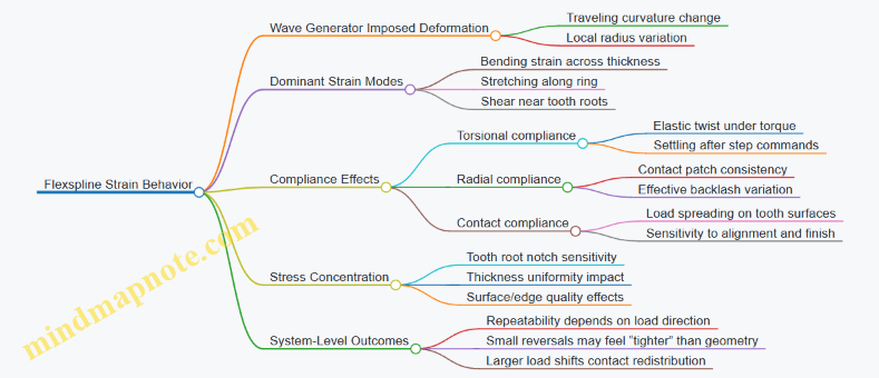
The wave generator imposes a traveling deformation on the flexspline. As that deformation moves, each flexspline tooth experiences a cycle of bending and stretching. The dominant strain modes are:
- Bending strain across the flexspline thickness, driven by the local curvature change.
- Membrane-like stretching along the ring, caused by the ring being forced into a different radius.
- Shear strain near the tooth roots and in the thin ligament regions, where the tooth geometry concentrates stress.
A useful mental model is to treat the flexspline as a thin ring with tooth “fingers.” The wave generator changes the ring’s local radius, so the tooth fingers must flex to maintain contact. If the tooth ligaments are too thick, the flexspline becomes stiff and the wave cannot form cleanly. If they are too thin, the teeth deform excessively and contact becomes inconsistent.
Compliance Effects on Motion
Compliance is not a defect; it is the mechanism that makes the reduction ratio possible. But compliance changes how the drive behaves under load.
- Torsional compliance: The flexspline twists elastically as torque transfers through the tooth engagement. This creates a small angular deflection between input and output.
- Radial compliance: The flexspline’s ability to change shape affects how consistently teeth stay in mesh. Under higher torque, the contact patch can shift, which slightly changes effective backlash.
- Contact compliance: Even when the flexspline geometry is fixed, the elastic deformation at the tooth surfaces spreads the load over a finite contact area. That spreading reduces peak stress but increases sensitivity to surface finish and alignment.
A concrete example: suppose you command a small step in position. If the flexspline is relatively compliant, the output will move, but the internal elastic twist will “wind up” and then settle as the tooth contact redistributes. The settling time depends on stiffness and damping, not just on your controller.
Stress Concentration and Tooth Root Behavior
Tooth roots are where strain energy likes to hide. The transition from tooth to base ring creates a geometry change, and that geometry change concentrates stress. Two manufacturing-related details strongly influence this:
- Thickness uniformity: Small thickness variations change local stiffness, so the wave deformation is not perfectly uniform.
- Surface and edge quality: Micro-roughness and tool marks can alter local contact pressure, which changes how much of the load goes through the tooth tip versus the root.
A practical example during machining: if a tool leaves a sharp burr at a tooth root, the burr can act like a tiny notch. The drive will still function, but the strain cycle becomes harsher at that location, increasing the chance of early fatigue.
Compliance vs Backlash and Repeatability
Backlash in harmonic drives is often discussed as a geometric gap, but flexspline compliance blurs the picture. When the wave generator engages, the flexspline deforms so that contact occurs even if there is nominal clearance. That means:
- Small reversals may show reduced “free play” because the elastic deformation takes up the gap.
- Larger load changes can shift the contact pattern, so repeatability depends on both load direction and magnitude.
A simple test setup: apply a constant torque, then command a small bidirectional oscillation. If repeatability degrades when you reverse direction, you are seeing compliance-driven contact redistribution rather than a purely geometric backlash issue.
Mind Map: Flexspline Strain and Compliance
Practical Design Implications
When designing or machining the flexspline, treat compliance as a controllable parameter. Increase stiffness by thickening the flexspline or reducing tooth ligament length, and you reduce elastic twist but risk poor wave formation and higher stress at contact. Reduce stiffness and you improve wave formation, but you increase elastic deflection and make the drive more sensitive to load-dependent contact shifts.
The best practice is to connect geometry choices to measurable behavior: torque-to-deflection under a known load, repeatability under bidirectional steps, and smoothness during engagement. If those checks line up with your expectations, the flexspline is doing its job—flexing enough to mesh, but not so much that the drive becomes a spring you didn’t ask for.
2.3 Cover Wave Generator Operation and Load Transfer Paths
A harmonic drive’s wave generator is the part that “writes” the motion into the flexspline. It does this by forcing a controlled deformation pattern into the flexspline, then letting the deformation travel around the circumference as the generator rotates. The key idea is that the wave generator is not merely a gear-like reducer; it is a deformation engine that creates a moving contact region.
Wave Generator Operation
The wave generator typically consists of a rigid elliptical cam (or equivalent geometry) and a bearing arrangement that allows the cam to rotate while maintaining its effective eccentricity relative to the flexspline. When the cam rotates, the eccentricity causes the flexspline to alternately bulge and relax around its circumference.
A practical way to picture the deformation: imagine a thin ring pressed by an off-center roller. At the “high” side of the ellipse, the ring is forced inward or outward (depending on design), and at the “low” side it is closer to its free shape. As the cam rotates, the location of maximum deformation moves with it.
Contact Region and Motion Transfer
The flexspline teeth engage the circular spline teeth only in the vicinity of the deformation maximum. That means the drive’s effective gearing action happens in a moving window rather than across the entire circumference. This moving window is what produces the reduction ratio: each full rotation of the wave generator advances the flexspline by a fraction of a turn determined by the tooth count relationship.
Why Deformation Must Be Controlled
If the flexspline deformation is uneven, tooth engagement becomes uneven too. That shows up as higher local stress, increased friction, and inconsistent backlash behavior. Good designs therefore aim for a predictable deformation shape by controlling flexspline thickness, material properties, and the wave generator’s eccentricity and surface finish.
Load Transfer Paths
Load transfer in a harmonic drive is a chain of cause-and-effect: motor torque creates generator reaction forces, those forces deform the flexspline, and the deformed flexspline transmits torque through tooth engagement to the circular spline.
Step-by-Step Load Path
- Input torque at the wave generator shaft creates a tangential force at the cam surface.
- Cam-to-flexspline normal force arises from the cam’s geometry and eccentricity. This normal force is the main driver of deformation.
- Flexspline bending and hoop strain distribute the load through the thin sections designed to flex. The flexspline is effectively a compliant structure with stiffness that depends on thickness and width.
- Tooth engagement forces occur where the flexspline teeth meet the circular spline teeth. These forces include tangential components (torque) and radial components (support).
- Circular spline reaction carries the load into its housing or output shaft.
A useful mental model is that torque is carried primarily by the engaged tooth pair(s) in the moving window, while the rest of the flexspline mainly provides the elastic “spring” that keeps the window traveling smoothly.
Force Components and Their Consequences
- Tangential component controls output torque. If it is too high for the tooth geometry and surface finish, you’ll see rapid wear and increased friction torque.
- Radial component affects stiffness and backlash. Too much radial load without adequate support can increase compliance variations, which can look like control jitter in a precision servo.
- Bending moment in the flexspline influences fatigue life. Even if torque seems acceptable, excessive bending from misalignment or poor fit can shorten life.
Integrated Example
Consider a compact drone gimbal joint where the harmonic drive must hold position under small disturbances. During operation, the wave generator rotates and the deformation maximum sweeps around the flexspline. The engaged tooth region moves, so the load is not applied uniformly at every angle.
If assembly alignment is slightly off, the deformation window may become biased toward one side. The result is that one portion of the tooth engagement carries more tangential and radial load. In practice, that can increase friction torque and create a repeatable position error pattern tied to the generator’s rotation angle.
A good diagnostic approach is to correlate measured friction or position ripple with generator angle. If the ripple frequency matches the wave generator’s rotation pattern, the issue likely sits in the load transfer geometry rather than in the motor electronics.
Mind Map: Wave Generator Operation and Load Transfer Paths
Quick Check for Understanding
If you can answer this in one sentence, you’ve got the core mechanism: the wave generator rotates, causing a controlled deformation maximum to travel around the flexspline, and the moving tooth engagement window is where torque is transferred from the generator to the circular spline while the flexspline provides the compliant spring path.
2.4 Analyze Backlash and Torsional Stiffness in Practice
Backlash and torsional stiffness are the two gremlins that show up when you try to command precise angles with a harmonic drive. Backlash is the “dead zone” between commanded and transmitted motion. Torsional stiffness is how much torque it takes to twist the drivetrain by a given angle. In practice, they trade off with geometry, preload, lubrication, and assembly quality.
What Backlash Means in a Harmonic Drive
Backlash is not just a single number; it depends on direction and load. In a harmonic drive, the flexspline and circular spline mesh through a wave generator. When torque reverses, the contact pattern shifts, and the system may rotate a small amount before the next tooth engagement path carries torque.
A practical way to measure backlash is to use a controlled reversal test: hold the input fixed, apply a small torque to the output in one direction until motion stabilizes, then reverse torque and record the output angle change before torque starts to rise again. If your sensor is on the output, you can directly observe the dead zone. If the sensor is on the motor side, you must account for compliance in the transmission and bearings.
How Torsional Stiffness Shows Up
Torsional stiffness is the slope of torque versus twist angle in the operating range. For control, stiffness matters because it sets how much the drivetrain “springs” under load. Low stiffness makes the closed-loop system work harder and can increase overshoot or steady-state error when friction and backlash are present.
In a harmonic drive, stiffness is influenced by flexspline thickness, tooth geometry, bearing fit, and preload. Even if backlash is small, a drivetrain can still feel soft if the flexspline strain dominates the compliance.
A Systematic Measurement Workflow
Start with a measurement plan that separates backlash from stiffness.
- Choose a torque level that is high enough to overcome static friction but low enough to avoid nonlinear contact changes. A good starting point is a torque that produces measurable motion within a few degrees.
- Measure stiffness first in a monotonic sweep. Apply increasing torque in one direction and record torque and angle. Fit a line to the central region to estimate stiffness.
- Measure backlash second using reversals. Keep the torque magnitude the same in both directions, reverse slowly, and record the angle gap between the last stable point in one direction and the first stable point in the other.
- Repeat at multiple torque levels. Backlash often changes with load because contact stiffness and friction change the effective engagement.
A simple sanity check: if your measured stiffness changes drastically with tiny torque variations, you may be measuring friction and contact hysteresis rather than elastic twist.
Mind Map: Backlash and Torsional Stiffness in Practice
Example: Reversal Test on a Small Output Shaft
Suppose you command an output angle using a servo that measures angle at the output. You perform a reversal test with a torque of 0.05 N·m.
- In the clockwise direction, you apply torque until the angle stabilizes at 12.40°.
- Then you reverse torque to 0.05 N·m counterclockwise.
- The output angle moves to 12.10° before torque begins to rise consistently.
The backlash gap is 0.30°. If you repeat the test at 0.10 N·m and the gap becomes 0.22°, you have evidence that backlash is load dependent. That matters for control: a controller tuned at one load may behave differently at another.
Example: Stiffness Sweep and Control Implications
Now run a monotonic sweep in the clockwise direction. At 0.02 N·m you measure 0.08° twist, and at 0.06 N·m you measure 0.24° twist. The slope is 0.24° / 0.06 N·m = 4° per N·m.
If your control loop commands a torque step that expects a certain angle response, but the drivetrain twist is larger than predicted, you’ll see a lagged angle response and potentially oscillation when the loop corrects. Increasing preload might reduce backlash, but stiffness depends on flexspline compliance and bearing/housing deformation, so you should not assume preload alone fixes everything.
Practical Best Practices That Improve Both Metrics
- Use consistent torque magnitude during reversals so backlash comparisons are meaningful.
- Control the direction of approach in tests; always approach the reversal point from the same prior condition.
- Check sensor placement and scaling. A small encoder offset can masquerade as backlash.
- Keep lubrication and temperature stable during measurement. Contact friction changes with viscosity, which changes the apparent dead zone.
- Verify assembly alignment. Misalignment can increase both hysteresis and effective compliance.
Backlash tells you how much motion you lose on reversals. Torsional stiffness tells you how much the system twists under load. When you measure them separately but under the same operating conditions, you get a drivetrain model that matches what your servo controller actually experiences.
2.5 Translate Gear Geometry into Machining and Inspection Needs
Gear geometry is not just a drawing exercise; it is a set of constraints that must survive tool access, fixturing, cutting mechanics, and measurement. The goal of this section is to convert geometric requirements into concrete machining steps and inspection checks, so the finished harmonic drive components mesh smoothly and repeatably.
Start with Geometry Requirements That Actually Matter
Begin by listing the geometry features that control function. For harmonic drive elements, the most common “must be right” items are: tooth profile form, tooth spacing and indexing accuracy, concentricity between functional axes, surface finish on mating faces, and thickness or diameter tolerances that affect engagement and stiffness. A practical habit is to annotate the CAD model with “functional surfaces” and “datums,” then carry those labels into process planning.
Example: if the flexspline tooth form must match a mating wave generator surface, the functional requirement is not “looks smooth,” but a specific profile accuracy and a surface finish that supports low friction during repeated flexing.
Map Each Geometry Feature to Machining Reality
Machining can only reproduce what the tool can reach and what the setup can hold. Translate each geometry feature into three machining questions: (1) what tool motion creates it, (2) what datum controls it, and (3) what error sources can distort it.
- Tooth profile form
- Machining translation: choose a toolpath strategy that follows the intended profile rather than approximating it with coarse steps.
- Error sources: tool radius compensation mismatch, feed marks, and deflection under cutting load.
- Inspection translation: measure profile deviation using a method aligned to the profile direction.
- Indexing and tooth spacing
- Machining translation: define the indexing method and the angular reference used during cutting.
- Error sources: backlash in indexing hardware, runout in the rotary axis, and inconsistent zeroing.
- Inspection translation: check angular spacing by measuring multiple tooth-to-tooth intervals.
- Concentricity and axis alignment
- Machining translation: select workholding datums that are stable and repeatable, then reference all critical features to those datums.
- Error sources: soft jaw deformation, part rocking, and thermal drift.
- Inspection translation: measure runout and concentricity at the functional diameters.
- Surface finish and micro-topography
- Machining translation: set finishing passes and cutting parameters that reduce tool marks on mating surfaces.
- Error sources: chatter, inconsistent tool wear, and interrupted cuts.
- Inspection translation: verify finish with a consistent measurement direction and location.
Choose Datums Early and Keep Them Consistent
Datums are the bridge between CAD, machining, and inspection. If you change datums midstream, you create a tolerance stack that no one can explain. A systematic approach is to define: a primary datum for axis location, a secondary datum for angular reference, and a tertiary datum for locating faces.
Example: when machining a circular spline seat, use the same axis datum for both cutting and measurement. If the inspection uses a different reference surface than the machining setup, the reported concentricity may be “correct” relative to the wrong axis.
Build a Geometry-to-Process Checklist
Use a checklist that forces every requirement into a machining and inspection action. This prevents the common failure mode where drawings specify tolerances but the process plan never states how they will be achieved.
- Feature: tooth profile
- Machining action: profile-following toolpath, finishing pass, controlled compensation
- Inspection action: profile deviation check at multiple angular positions
- Feature: tooth spacing
- Machining action: calibrated indexing, verified zero repeatability
- Inspection action: angular interval measurement across the tooth set
- Feature: concentricity
- Machining action: stable fixturing datums, minimize runout
- Inspection action: runout measurement at functional diameters
- Feature: surface finish
- Machining action: finishing parameters, tool wear monitoring
- Inspection action: finish measurement at defined locations and direction
Mind Map: Geometry to Machining and Inspection
Example: From CAD Tolerance to Shop Checks
Suppose the circular spline requires a tight concentricity between the bearing seat and the spline axis. The translation is:
- Machining: cut the bearing seat first using the primary axis datum, then machine spline features without re-clamping to a different reference. If re-clamping is unavoidable, add a re-zero step and verify repeatability.
- Inspection: measure runout at the bearing seat and at the spline functional diameter using the same axis reference. If the two runout readings disagree, the issue is not “the part is bad,” it is “the reference chain is broken.”
Example: Tooth Profile Form with Tool Access Limits
If the flexspline tooth profile is specified tightly, tool access may prevent a single-pass strategy. The translation is:
- Machining: use a multi-step approach that maintains the intended profile direction, then finish with a pass that targets the mating surface.
- Inspection: check profile deviation after finishing, not after roughing, because roughing can leave geometry errors that finishing cannot fully remove.
Close the Loop with In-Process Verification
Finally, inspection should not be a surprise at the end. Add in-process checks at points where geometry is still adjustable: after roughing but before finishing, after any re-clamping, and after tool changes that affect surface finish. The best inspection plan is the one that catches the error while it is still cheap to fix.
3. Precision Servo Architectures for Small Actuators
3.1 Compare Common Servo Layouts for Robotics and Drones
Servo layout choices determine how torque, stiffness, and sensing errors show up at the output shaft. In practice, you’re balancing four things: where the reduction happens, how the motor and load are aligned, how backlash and friction are managed, and how much wiring and mass you can tolerate.
Foundational Layout Types
Direct-Drive With High-Torque Motor places the motor close to the joint and uses little or no gear reduction. This layout is simple to assemble and often gives smooth motion, but it usually demands a larger motor and stronger power electronics to achieve the same torque at low speed. A common example is a small pan-tilt stage where the joint torque is modest and the control loop can handle higher motor inertia.
Geared Servo With Motor Near the Joint uses a compact gearbox between motor and output. Reduction lowers motor speed and current for a given joint torque, which helps with efficiency and thermal headroom. The tradeoff is that gear mesh introduces compliance and backlash, so you must design the control strategy around measurable friction and deadband.
Remote-Motor With Belt or Shaft Transmission moves the motor away from the joint to save space or reduce heat near sensitive components. The transmission adds torsional windup and can complicate calibration because the measured position may not represent the joint angle directly. A typical use case is a drone where the motor sits in a fuselage bay and the joint is at the wing or tail.
Harmonic-Drive Style Reduction uses a flexspline strain wave mechanism to achieve high reduction in a compact package. It can provide low backlash, but it still has torsional compliance and friction that vary with preload and temperature. This layout is often chosen when you need high ratio without a large gearbox footprint.
How Layout Affects Control Behavior
Start with the output equation you care about: joint torque versus joint angle under load. If reduction is high, motor current changes become a smaller fraction of output torque, which can make tuning feel “stiffer” at the joint but “softer” at the motor side. If the motor is remote, the transmission adds an extra spring, so the control loop may see phase lag and overshoot unless you measure or model that compliance.
Backlash shows up differently depending on where it lives. In a geared layout, backlash can create a dead zone in output motion when reversing direction. In a remote layout, backlash plus belt elasticity can create a delay-like effect that looks like sluggishness rather than a clean deadband.
Practical Comparison Criteria
Use the same checklist for each candidate layout:
- Stiffness at the Output: Higher stiffness reduces tracking error under disturbances.
- Backlash and Friction: Low backlash helps repeatability, but friction still affects steady-state error.
- Sensing Placement: If the sensor measures motor position, you must account for transmission compliance; if it measures joint position, wiring and packaging get harder.
- Thermal Path: Motor placement changes how quickly torque can be sustained.
- Assembly Tolerance Sensitivity: Misalignment and concentricity errors can dominate small-part performance.
Mind Map: Servo Layout Decision Flow
Concrete Examples with Reasoned Tradeoffs
Example: Drone Gimbal Pitch Joint
- If the joint must hold attitude against wind gusts, output stiffness matters more than maximum speed.
- A geared servo near the joint reduces motor current and keeps wiring short.
- If you place the encoder at the joint, you avoid having to estimate belt or gear compliance, which simplifies tuning.
Example: Robotic Arm Wrist Rotation
- The wrist often needs fast direction changes and repeatable positioning.
- A harmonic-drive style reduction can reduce backlash, improving reversal behavior.
- You still need to manage friction and preload consistently during assembly, because small changes alter the torque required to start motion.
Example: Drone Tail Actuation With Space Constraints
- If the motor must sit away from the tail for mass and airflow reasons, remote transmission becomes attractive.
- Expect torsional windup and phase lag, so the control loop benefits from either joint sensing or a model-based compensation approach.
Summary Comparison
Direct-drive layouts prioritize simplicity and smoothness but often require bigger motors. Geared layouts near the joint balance compactness with manageable backlash. Remote layouts trade packaging for compliance that must be handled in sensing and control. High-ratio wave reduction targets compact torque with low backlash, at the cost of preload-sensitive friction and compliance that you must treat as part of the system, not an afterthought.
3.2 Select Motor Types and Match Them to Gear Reduction
Choosing a motor for a harmonic drive or precision servo is mostly about matching torque and speed to what the gear train can actually deliver. The gear reduction changes the relationship between motor torque and output torque, but it does not magically remove limits like motor current, thermal rise, bearing friction, or control bandwidth. A good match starts with the output requirements, then works backward through reduction, efficiency, and inertia.
Step 1: Define Output Requirements in Plain Numbers
Start with steady torque and motion profile, not just peak torque. For example, if a drone gimbal needs 0.25 N·m to hold position and 0.40 N·m during a fast slew, treat those as separate design points. Also note required output speed: if you need 120 °/s output, convert to rad/s and keep it consistent across calculations.
Step 2: Convert Output Torque to Required Motor Torque
For a harmonic drive, the ideal relationship is:
- Motor torque ≈ Output torque / reduction / efficiency
Use a realistic efficiency for your configuration and lubrication state. If you assume 60:1 reduction and 0.75 efficiency, then for 0.40 N·m output:
- Motor torque ≈ 0.40 / 60 / 0.75 ≈ 0.0089 N·m
That number tells you the motor must supply about 9 mN·m at the motor shaft during the demanding segment. If your motor’s torque constant and current limits cannot reach that torque without overheating, the mismatch will show up as sluggish motion or thermal shutdown.
Step 3: Convert Output Speed to Motor Speed
Gear reduction multiplies speed in the opposite direction:
- Motor speed ≈ Output speed × reduction
If output is 120 °/s (2.094 rad/s) and reduction is 60:1, motor speed is about 126 rad/s or 1200 rpm. This matters because many motors can produce rated torque only up to a speed where back-EMF and voltage limits take over.
Step 4: Choose Motor Type by Where Its Limits Live
Different motor types fail in different ways, so the “best” choice depends on whether your constraints are current-limited, voltage-limited, or control-limited.
Brushless DC (BLDC) servo motors are a common fit for precision servos because they provide smooth torque with closed-loop commutation and strong torque density. They are often current-limited at low-to-mid speeds and voltage-limited at higher speeds. If your required motor speed is moderate and you need crisp torque control, BLDC is usually a straightforward match.
Coreless DC motors can be excellent for low inertia and high responsiveness. Their low rotor inertia helps the control system react quickly to disturbances, which is useful when the load inertia changes with mounting orientation. The tradeoff is typically cost and sometimes lower continuous torque capability compared with larger-frame options.
Stepper motors can work when the motion is mostly open-loop or when you can accept torque ripple and resonance management. With harmonic drives, the high reduction can help reduce output ripple, but it does not remove motor detent torque effects at the motor shaft. If you need tight position repeatability under varying loads, steppers often require careful current control and damping.
Pancake and ironless variants are often chosen for compactness, but the same rule applies: check torque constant, thermal limits, and maximum speed. A thin motor that fits the envelope can still be unusable if its continuous current is too low for your required motor torque.
Step 5: Match Motor Inertia to Gear Train and Control Bandwidth
Even with perfect torque numbers, the motor and gear train inertia affect how quickly the servo can correct errors. A practical rule is to keep the motor’s reflected inertia from dominating the load inertia at the frequencies you care about. If the motor inertia is too high, the controller may need more gain to achieve the same response, which can amplify noise and saturate current.
Step 6: Use a Simple Selection Workflow
A reliable workflow prevents “it fits on paper” surprises.
- Compute motor torque from output torque using reduction and an efficiency assumption.
- Compute motor speed from output speed using the same reduction.
- Check motor torque at that speed against continuous and peak current limits.
- Check voltage headroom for the motor’s back-EMF at that speed.
- Confirm thermal rise is acceptable for your duty cycle.
- Verify that motor inertia and gearbox friction do not exceed what your control loop can handle.
Mind Map: Motor Type Selection and Gear Reduction Matching
Example: Matching a BLDC Motor to a 60:1 Harmonic Drive
Assume a gimbal needs 0.25 N·m holding torque and 0.40 N·m during slews, with 120 °/s output speed. Using 60:1 reduction and 0.75 efficiency:
- Motor torque for slew ≈ 0.0089 N·m
- Motor speed ≈ 1200 rpm
If a candidate BLDC motor has a torque constant of 0.03 N·m/A, then required current for slew torque is about 0.0089 / 0.03 ≈ 0.30 A. That current is plausible, but you still check whether the motor can sustain it at the required speed without exceeding voltage limits and thermal rise. If the motor’s driver voltage is insufficient at 1200 rpm, the motor will produce less torque than expected, and the gimbal will lag during fast moves.
Example: When a Coreless Motor Makes Sense
If the same gimbal must reject quick disturbances from prop wash or cable motion, low rotor inertia can reduce the time the controller spends “chasing” the error. Even if the torque requirement is similar, the coreless motor’s lower inertia can improve settling time because the motor accelerates the reflected load more readily. The selection still depends on continuous torque and thermal limits, but the dynamic advantage can be real when response time is the key requirement.
Example: Stepper Choice for Lower-Speed, High-Repeatability Moves
If the output speed is modest and the motion is mostly point-to-point with minimal disturbance torque, a stepper with microstepping can be adequate. The harmonic drive reduction helps reduce output step size, but you must ensure the motor can hold the required torque without losing steps under friction and compliance. In practice, the “match” is less about peak torque and more about whether the stepper stays synchronized through the full motion profile.
The core idea is simple: compute what the motor must do at its own shaft, then pick the motor type whose limits align with your operating point and whose dynamics your controller can manage.
3.3 Choose Sensors and Feedback Topologies for Position Control
Position control lives or dies by what you measure and how quickly you can measure it. For miniaturized harmonic drives and precision servos, the sensor choice should match the dominant error sources: motor-side commutation errors, gear-train compliance, backlash, and friction that changes with load and temperature.
Start with a simple mental model: the controller wants a mapping from command position to actual output position. If the sensor is on the motor shaft, the controller sees motor motion but not the gear-train effects directly. If the sensor is on the output shaft, the controller sees the result of everything in between, but you pay in packaging, wiring, and sometimes measurement resolution.
Foundational Sensor Placement
There are three common placement strategies.
-
Motor-side sensing measures rotor angle or motor shaft position. This is straightforward and often high resolution. The downside is that gear compliance and backlash become “invisible” disturbances.
-
Gear-train intermediate sensing measures after some reduction stage. This can reduce the impact of motor-side disturbances while keeping the sensor easier to package than an output-shaft sensor.
-
Output-side sensing measures the final shaft angle. This directly closes the loop around backlash and compliance effects, improving repeatability when the mechanism is well assembled.
A practical rule: if your application cares most about output accuracy under varying load direction, output-side sensing is usually worth the extra effort. If your application cares most about smooth motion and you can keep loads consistent, motor-side sensing can be sufficient.
Feedback Topologies That Match the Physics
A topology is how you combine sensor signals with control loops.
-
Single-loop position control uses one position sensor and computes the position error. It’s conceptually clean and works well when the sensor is on the output or when disturbances are small.
-
Cascaded loops use an inner loop for current or velocity and an outer loop for position. The inner loop handles fast dynamics; the outer loop handles slower position correction. This reduces the burden on the position loop and helps the system stay stable.
-
Hybrid sensing combines motor-side and output-side information. A common approach is to use motor-side sensing for fast response and output-side sensing to correct steady-state errors and backlash effects.
When backlash exists, a single-loop controller can “hunt” around the dead zone if the sensor is motor-side. Output-side sensing reduces that hunting because the controller sees the actual output movement.
Sensor Types and What They Measure Well
Incremental encoders provide high resolution and good bandwidth. They require careful index handling at startup and can be sensitive to electrical noise in small enclosures. They are excellent for velocity estimation in cascaded loops.
Absolute encoders provide position without a homing routine. They simplify startup and reduce the chance of losing track after power cycles. The tradeoff is often lower resolution per cost tier and more complex wiring.
Resolvers are robust in noisy environments and can be easier to integrate with some motor types. Their angle accuracy depends on excitation and signal conditioning quality.
Hall sensors are typically used for commutation and coarse position. They rarely provide the resolution needed for tight output positioning unless paired with a higher-resolution sensor.
Potentiometers can work for low-cost prototypes but are usually limited by wear, nonlinearity, and mechanical stability. In miniaturized mechanisms, their wiper alignment can become a hidden source of drift.
Mind Map: Sensor and Topology Selection
Systematic Selection Workflow
-
List the dominant error sources: backlash, torsional compliance, friction, and sensor quantization. If backlash is significant, prioritize output-side sensing or hybrid sensing.
-
Check bandwidth requirements: if you need quick settling, ensure the sensor and interface support the loop rates. Incremental encoders often excel here.
-
Match sensor resolution to control needs: quantization noise shows up as limit-cycle motion. If your controller step size is smaller than the sensor’s effective resolution, you’ll waste effort.
-
Validate mechanical mounting: runout and misalignment between encoder and shaft can create angle ripple that the controller interprets as motion. A stiff mount and controlled concentricity matter as much as sensor specs.
-
Plan signal conditioning: differential encoder signals and proper grounding reduce noise-induced jitter. In small builds, cable routing and shielding can be the difference between “works on the bench” and “works in the drone.”
Example: Choosing Between Motor-Side and Output-Side Encoders
Suppose you’re building a compact servo for a robotic link that reverses direction frequently. With motor-side incremental sensing, the controller sees rotor angle changes immediately, but the output lags while the harmonic drive takes up compliance and backlash. You’ll often observe a small overshoot or slow correction when the direction changes.
If you move the sensor to the output shaft, the controller directly measures the lag and dead zone behavior. The same cascaded control structure can then correct position based on what the mechanism actually does, improving repeatability. If packaging makes output sensing difficult, a hybrid approach can still help: use motor-side sensing for fast inner-loop control and output-side sensing for the outer position loop.
Example: Hybrid Topology with Backlash Compensation by Measurement
In a hybrid setup, the inner loop uses motor-side encoder feedback to regulate velocity tightly. The outer loop compares the commanded output angle to the output sensor reading. This arrangement keeps the fast dynamics stable while letting the outer loop correct the slow, direction-dependent errors introduced by the gear train.
The key is to avoid fighting the same error twice. If the outer loop is too aggressive, it can reintroduce hunting around backlash. If it’s too weak, the system behaves like motor-side control. The sensor placement and loop gains should be tuned together, using the output sensor as the truth source for settling behavior.
3.4 Build a Practical Control Stack from Measurement to Actuation
A practical control stack is just a chain of decisions that turns sensor readings into actuator commands. The trick is to make each link measurable, testable, and small enough that you can debug it without a full-body shrug.
Step 1: Define Signals and Units
Start by writing down every signal with units and expected ranges: position (rad or deg), velocity (rad/s), current/torque (A or N·m), and time (s). If your encoder outputs counts, decide the conversion to radians early and keep it consistent. A common “small” mistake is mixing degrees in the controller with radians in the plant model; it usually shows up as a controller that feels like it’s fighting itself.
Example: If the encoder is 2048 counts per revolution and you use radians, then
- angle_rad = counts * (2π / 2048)
- velocity_rad_s comes from a filtered derivative of angle_rad over time.
Step 2: Choose the Measurement Path
You typically need two measurement paths: one for the control variable (position or velocity) and one for disturbance estimation (often current or torque proxy).
Best practice: filter only what you must. Filtering position too aggressively adds phase lag, which makes tuning harder. A simple approach is:
- Use a low-pass filter on velocity (derived from position).
- Keep position lightly filtered or not filtered if your encoder is clean.
Concrete example: If your position signal has quantization steps, compute velocity using a difference over a short window (e.g., 2–5 samples) and then apply a first-order low-pass filter to reduce noise.
Step 3: Implement State Estimation When Needed
If you can measure velocity directly with a tachometer, great. If not, estimate it. For many small servo systems, a velocity estimate from filtered position is enough. For tighter performance, use a simple observer that blends a model with measurements.
Practical rule: start with the simplest estimator that produces stable control. If you later add an observer, keep the interface the same: the controller should still receive “estimated velocity” in consistent units.
Step 4: Build the Feedback Controller
A common baseline is a cascaded structure:
- Outer loop: position controller outputs a velocity or torque demand.
- Inner loop: velocity or current controller drives the actuator.
For harmonic drives, friction and compliance can cause steady errors and sluggish response if you only use position feedback. Adding a velocity loop helps because it reacts to motion error rather than only to final position error.
Example cascade:
- Position loop: PID (or PI) producing velocity demand.
- Velocity loop: PI producing torque/current demand.
Keep integrators under control. Use anti-windup so the integrator doesn’t accumulate when the actuator saturates.
Step 5: Add Feedforward That Actually Helps
Feedforward reduces the burden on feedback. Use it when you have a reliable reference trajectory.
Two practical feedforward terms:
- Velocity feedforward: helps with friction and damping.
- Torque feedforward: if you can estimate required torque from load and gear ratio.
Example: If your reference is a smooth sinusoid, you can compute desired acceleration and estimate torque proportional to inertia. Even a rough inertia estimate often improves tracking because the controller spends less time “catching up.”
Step 6: Handle Saturation, Rate Limits, and Safety
Actuators have limits: maximum current, maximum voltage, maximum command rate. Put these constraints between controller output and the motor driver.
Best practice: saturate the command, then adjust integrators or demands so the system doesn’t keep requesting impossible values.
Example: If torque demand exceeds the current limit, clamp it and freeze or back-calculate the integrator term in the velocity loop.
Step 7: Close the Loop with a Test Plan
Before tuning, verify timing and scaling:
- Confirm control loop period is stable.
- Confirm sensor conversion is correct.
- Confirm command-to-actuator mapping is correct.
Then tune in layers:
- Tune inner loop first (current/torque or velocity).
- Tune outer loop second (position).
- Add feedforward last.
Use step tests and small-amplitude sine tests. A step reveals overshoot and damping; a sine reveals phase lag and friction-induced distortion.
Mind Map: Measurement to Actuation Control Stack
Example: Minimal Working Control Stack for a Small Servo
- Read encoder counts, convert to angle_rad.
- Estimate velocity_rad_s from angle_rad over a short window, then low-pass filter.
- Position controller computes velocity_demand.
- Velocity controller computes torque_demand.
- Apply saturation to torque_demand and anti-windup.
- Convert torque_demand to current command using motor torque constant and gear ratio.
- Send current command to the driver, then log signals for tuning.
This structure keeps the interfaces clean: measurement outputs feed estimation, estimation feeds control, and control feeds constrained actuation. Once it runs, you can tune each block without rewriting the whole system—like fixing one gear tooth at a time instead of rebuilding the gearbox.
3.5 Define Mechanical and Electrical Integration Requirements
Mechanical and electrical integration requirements are where “it works on the bench” becomes “it works in the robot.” For miniaturized harmonic drives and precision servos, the integration spec must connect geometry, motion, and signals into one consistent set of constraints.
Mechanical Integration Requirements
Start with the motion path and work outward. Define the output interface first: shaft diameter, keying or spline type, allowable axial play, and the maximum permitted radial runout at the mating surface. For example, if a gimbal joint expects a 6.00 mm shaft with ±0.01 mm runout, your gearbox output must be measured at the same reference plane used by the gimbal bearing.
Next, specify the housing and alignment strategy. Harmonic drives are sensitive to misalignment because the flexspline and circular spline share load through mesh. A practical requirement is to limit angular misalignment between the wave generator axis and the output axis. If you do not have a direct measurement method, require a surrogate: concentricity of bearing seats and perpendicularity of mounting faces.
Then define fastener and preload behavior. Small assemblies often fail from “almost right” torque. Write the requirement as a torque range plus a seating procedure: for instance, tighten in two stages, verify that the wave generator housing seats flush, and confirm that the output rotates freely before final torque. Add a requirement for thread engagement length and fastener material to prevent loosening under vibration.
Finally, include cable and strain relief constraints. A servo cable that flexes at the connector can create intermittent encoder faults. Specify bend radius, minimum cable length to the first tie point, and a strain relief method that does not load the connector shell.
Electrical Integration Requirements
Electrical requirements should be stated in terms of signals, timing, and protection. Begin with the sensor interface: encoder type, resolution, output format (differential or single-ended), and expected supply voltage. If the encoder is differential, require twisted pair routing and a defined termination scheme at the controller side.
Define motor drive electrical limits. Specify phase current range, bus voltage tolerance, and allowable peak current duration. For a concrete example, if the controller can supply 2.0 A peak but the motor winding is rated for 1.6 A continuous, you must state the current limit and the controller’s current loop bandwidth so the drive does not overshoot during startup.
Now address grounding and shielding. Require a single-point reference strategy or a defined chassis connection method. For small systems, the most common integration bug is ground loops that shift encoder thresholds. State the requirement: shield termination at the controller end, motor phase wiring kept separate from encoder wiring for a defined distance, and no shared return paths for encoder current.
Add protection requirements that match the mechanical reality. If the gearbox assembly can experience occasional stall torque, specify overcurrent and overtemperature behavior in the controller. Also require connector pinout verification and keyed mating to prevent swapped phase leads.
Integrated Interface Checklist
Use one checklist that ties mechanical and electrical constraints together.
- Output shaft interface: diameter, runout reference plane, axial play limit.
- Mounting geometry: face perpendicularity, bearing seat concentricity, alignment method.
- Assembly procedure: torque stages, seating verification, free-rotation check.
- Cable routing: bend radius, tie points, strain relief, connector loading limits.
- Encoder interface: signal type, voltage, termination, routing separation.
- Motor drive: current limits, bus tolerance, startup behavior.
- Grounding: shield termination rule, return path definition.
- Protection: stall/overcurrent/thermal response behavior.
Mind Map: Mechanical and Electrical Integration
Example: Integration Spec for a Compact Robotic Joint
A robotic elbow joint uses a harmonic drive reduction and a 20-bit encoder on the motor side.
- Mechanical: output shaft 6.00 mm with runout ≤ 0.01 mm measured at the joint bearing seat; mounting faces perpendicular within 0.02 mm over the bolt circle; torque fasteners in two stages (50% then 100%) and verify free rotation before final torque.
- Electrical: encoder differential outputs, 5 V supply, twisted pair routing with shield termination at the controller end; motor phase wiring separated from encoder lines by at least 15 mm along the harness; controller current limit set to 1.6 A continuous equivalent with defined peak duration; overcurrent trips within 50 ms to prevent repeated stall chatter.
This kind of integrated spec prevents the classic mismatch where the mechanical assembly meets tolerances but the controller wiring quietly changes the encoder signal quality.
4. Subtractive Manufacturing Tooling and Setup for Small Parts
4.1 Choose Machine Tools and Fixturing Approaches for Miniatures
Miniature harmonic drives and precision servos punish sloppy setups. A flexspline tooth might be only a few tenths of a millimeter wide, so the machine tool and fixturing must deliver repeatable geometry, not just “good enough” parts. The goal is simple: control the workpiece position in all relevant degrees of freedom, then keep it stable while cutting forces and thermal effects do their thing.
Foundations: What Miniature Machining Must Control
Start by listing the error sources you can’t afford:
- Workpiece location errors: wrong center, tilted axis, or inconsistent height.
- Runout and concentricity errors: tool or spindle wobble, loose clamping, uneven seating.
- Tool deflection: small tools flex more relative to their size.
- Thermal drift: the part warms, the fixture warms, and the reference shifts.
A practical way to connect these to machine choice is to ask: “How will I measure and correct the work coordinate system (WCS) every time?” If you can’t reliably re-establish WCS, the machine’s nominal accuracy won’t matter.
Machine Tool Selection: Capabilities That Actually Matter
Spindle and Speed Control
For small cutters, surface finish and dimensional stability depend on consistent spindle speed and low vibration. Look for:
- Stable speed under load so tooth features don’t smear.
- Low runout at the spindle nose so circular features stay circular.
Example: If you’re machining a wave generator surface with a small end mill, speed variation can show up as waviness that later assembly can’t fix.
Rigidity and Tool Overhang
Miniature work often uses short tools, but tool overhang still happens with reach requirements. Choose a machine with:
- Rigid tool holders and predictable clamping.
- Enough spindle bearing stiffness to resist deflection.
Example: Two machines can both “cut the same material,” but the one with higher stiffness will hold tooth flank angles closer to the programmed profile.
Axis Accuracy and Motion Quality
You care about more than positioning resolution. Motion quality affects:
- Interpolation smoothness for curved tooth paths.
- Repeatability when you re-zero after tool changes.
Example: When cutting a circular spline interface, poor motion quality can create subtle chord errors that become backlash later.
Work Envelope and Access
Fixturing for small parts needs clearance for:
- Tool approach angles
- Chip evacuation
- Probe access for in-process measurement
Example: A compact fixture that blocks the probe can force you into “measure later” habits, which increases scrap.
Fixturing Approaches: Repeatability over Heroics
Fixturing is the part of the system that most often ruins good machining plans. The best fixturing approach is the one that makes re-clamping predictable.
Reference Strategy: Where Is Zero?
Pick a primary datum and stick to it:
- Primary datum: the surface that defines height and most of the orientation.
- Secondary datum: the surface that defines rotation about the primary.
- Tertiary datum: the surface that prevents rocking.
Example: For a flexspline blank, using a ground outer cylinder as the primary datum and a flat as the secondary datum helps keep thickness-related features consistent.
Clamping Method: Avoid Distorting the Part
Small parts can deform under clamp force. Prefer:
- Soft jaws shaped to the part geometry.
- Low-force, high-repeatability clamping where possible.
- Support under thin sections to prevent bending.
Example: Over-tightening a collet on a thin ring can change the local thickness, and the machined tooth geometry will reflect that distortion.
Locating Features and Repeatability
Use features that constrain the part without relying on “feel”:
- Close-tolerance pins or bushings for repeat location.
- Shoulders for consistent seating.
- Kinematic-style locating when you need high repeatability.
Example: A small shoulder plus a single locating pin can outperform a “tighten until it looks right” approach by removing guesswork.
Chip Control and Contact Surfaces
Miniature machining needs clean contact surfaces:
- Chip traps and shields to keep grit off reference faces.
- Regular cleaning of locating surfaces.
Example: A single chip under a datum face can shift the part by more than your inspection tolerance.
Mind Map: Machine Tool and Fixturing Decision Flow
Example Workflow: From Setup to Verified Cutting
- Dry-fit the fixture and confirm probe clearance for the datums you will measure.
- Define datums on the part and fixture, then program WCS based on those datums.
- Probe the primary and secondary datums after each re-clamp to confirm repeatability.
- Run a short “first-article” cut on a non-critical area to check surface quality and dimensional response.
- Inspect concentric features early, because correcting a bad datum later is expensive.
This workflow keeps the system honest: if the machine is accurate but the fixture can’t re-establish the same reference, the part will still miss.
Practical Checklist for Small Parts
- Can you re-establish WCS after tool changes without manual guessing?
- Does the fixture support thin sections without bending them?
- Are chip paths designed so reference faces stay clean?
- Do you have a probe or measurement method that can validate datums quickly?
- Is the machine rigid enough for your tool diameter and required reach?
If you can answer “yes” to these, you’ve chosen a machine tool and fixturing approach that supports miniature accuracy instead of fighting it.
4.2 Select Cutting Tools and Determine Practical Cutting Parameters
Selecting tools and parameters for tiny, subtractively manufactured harmonic-drive components is mostly about controlling three things: how the tool contacts the work, how much heat you create, and how repeatable your results are from part to part. The goal is not maximum speed; it’s stable cutting that preserves geometry and surface finish.
Tool Selection Foundations
Start with the material state you’re actually cutting. If you’re machining a flexspline blank, you often care about uniform thickness and minimal distortion, so tool choice should prioritize dimensional stability and consistent chip formation. For circular spline and bearing interfaces, tool choice should prioritize accuracy at shoulders and seats.
Next, match tool geometry to the feature. Small tooth forms and bearing seats punish tools that are too blunt or too aggressive. A sharp edge with predictable runout tolerance matters more than exotic coatings. If your machine is small and your workholding is compact, you also need a tool that can reach the feature without excessive stickout.
Finally, decide how you’ll manage chips. In miniature gear work, chips that don’t clear can re-cut and smear, which ruins surface finish and can seed burrs that later interfere with assembly.
Cutting Parameter Logic
Cutting parameters are a chain: spindle speed sets cutting velocity, feed per tooth sets chip thickness, and depth of cut sets cutting forces and tool deflection. When any link is wrong, the chain breaks as chatter, burrs, or poor finish.
A practical workflow is to begin with a conservative starting point, then adjust one variable at a time while watching three signals: sound and vibration, chip appearance, and measured surface finish.
Speed and Feed Starting Points
Use the tool manufacturer’s recommended range as a ceiling, not a target. For small tools, the limiting factor is often tool deflection and heat at the cutting edge. If you see a shiny burnished surface, you’re likely rubbing too much; if you see rough tearing, you may be feeding too fast for the tool’s edge strength or chip evacuation.
A simple rule for first trials: keep depth of cut modest and use a feed that produces continuous chips rather than dust. Continuous chips are your evidence that the tool is cutting, not polishing.
Depth of Cut and Stepovers
For thin or flexible parts, depth of cut should be small enough to avoid bending the work during cutting. Stepovers should be chosen to maintain surface finish without overloading the tool laterally. If you’re finishing tooth-adjacent surfaces, smaller stepovers reduce scallop height and help you hit inspection targets.
Toolpath Strategy
Toolpath affects effective cutting load. Climb milling generally improves surface finish and reduces rubbing, but only if your setup is rigid enough. Use ramp entry or controlled lead-ins to avoid sudden engagement that can chip the tool.
For pocketing or roughing, leave a finishing allowance that your finishing pass can remove cleanly. If you try to finish from rough stock, you’ll chase errors with parameters instead of geometry.
Tool Wear and Inspection During Setup
Miniature tools can lose sharpness quickly, and wear changes your effective cutting parameters. Plan a short test cut, then inspect. Look for edge rounding, burr formation, and changes in surface texture.
When you adjust parameters, do it with a reason. If chips are short and powdery, increase feed or reduce speed slightly. If chips are long and stringy, reduce feed or increase chip evacuation effectiveness. If you see chatter marks, reduce depth of cut and improve rigidity or tool engagement.
Mind Map: Tool and Parameter Selection
Example: Flexspline Tooth Machining Trial
Assume a small end mill is used to generate tooth-adjacent surfaces on a flexspline blank. Begin with a conservative spindle speed and a feed that produces continuous chips. Use a shallow depth of cut to avoid bending the blank during engagement. Keep stepovers small enough that the finishing pass can remove scallops without excessive lateral load.
After the first test, inspect three things: (1) surface texture for signs of rubbing, (2) burr presence at tooth edges, and (3) any measurable change in thickness uniformity near the machined region. If burrs appear, reduce feed slightly or improve tool sharpness and entry strategy. If the surface looks smeared, reduce speed and confirm coolant or air blast effectiveness.
Example: Bearing Seat and Shoulder Cutting
For bearing seats, the priority is concentricity and shoulder sharpness. Choose a tool that can reach the seat with minimal stickout, and use a finishing pass with controlled depth of cut. If you rough too aggressively, the finishing tool must remove uneven material, which increases the chance of tool deflection and seat waviness.
Start with a speed/feed combination that yields clean chips and a stable finish. Use a consistent approach angle so the tool engages smoothly at the shoulder. After machining, measure seat diameter and shoulder location, then adjust parameters only if the surface finish indicates rubbing or if burrs indicate excessive edge load.
Practical Parameter Checklist
- Tool stickout minimized for rigidity.
- Conservative speed to prevent edge overheating.
- Feed chosen to create continuous chips.
- Modest depth of cut for thin or compliant parts.
- Small stepovers for tooth-adjacent finishing.
- Controlled lead-ins to prevent tool edge chipping.
- Short test cut followed by chip, finish, burr, and dimensional checks.
4.3 Plan Workholding for Repeatable Concentricity and Runout
Repeatable concentricity and low runout start long before the first cut. Workholding is the part of the process that quietly decides whether your machining results look consistent across parts—or like each part had a different mood.
Foundational Concepts That Drive Workholding Choices
Concentricity is about how well two features share a common axis. Runout is about how much a feature varies as it rotates. In small harmonic-drive components, the axis you think you’re using is often not the axis the machine actually sees. Workholding planning therefore focuses on three things: where the part’s reference axis is defined, how that reference is constrained, and how the constraints behave under cutting forces.
A practical rule: pick one datum axis for the entire setup chain. For example, if you will later machine flexspline features relative to a central bore, then the bore (or a temporary pilot) must be the primary reference during every operation that affects concentricity.
Step 1: Choose Datums and Define the Setup Chain
Start by listing the features that must be coaxial. Then decide the earliest feature you can reliably reference with your available tools.
- If the part already has a pilot bore from a prior operation, use it as the primary datum.
- If it does not, plan a temporary pilot strategy such as a soft center, a sacrificial boss, or a controlled drilling step that creates a reference you can later remove.
Next, map which operations must share the same axis. If an operation changes the reference axis, treat it as a new setup and plan a re-referencing method.
Step 2: Select a Workholding Strategy That Matches the Geometry
For miniaturized parts, the “best” workholding is usually the one that minimizes overconstraint and allows predictable seating.
-
Soft Jaws or Custom Inserts
- Use when the part has irregular outer geometry.
- Best practice: seat the part against a defined face and clamp radially with controlled pressure.
- Example: For a thin-walled ring, clamp on a thicker land rather than the thin section to avoid bending that later shows up as runout.
-
Collets and Precision Chucks
- Use when you can grip a cylindrical surface with enough length.
- Best practice: ensure the gripping surface is clean and free of burrs; even a small burr can create a repeatable but wrong axis.
- Example: When machining a circular spline seat, grip on a turned land and keep the land length consistent across parts.
-
Mandrels and Backing Supports
- Use when the part is too delicate to clamp directly.
- Best practice: support the part near the cutting zone to reduce deflection.
- Example: For flexspline blanks, use a mandrel that contacts a reference surface and provides axial support so the part doesn’t “float” under tool pressure.
Step 3: Control Seating, Clamp Force, and Overconstraint
Repeatability fails when the part can settle differently each time. Plan for consistent seating by using hard stops, locating shoulders, or a defined face contact.
Overconstraint is the silent enemy: if you clamp in a way that forces multiple points to match imperfect surfaces, the part may rock slightly, producing runout.
- Use one primary radial constraint and one axial constraint.
- Allow compliance where appropriate, such as using a soft interface layer (for example, a thin shim stack) only if it is controlled and repeatable.
Example: If you clamp a ring by both inner and outer diameters, but the inner diameter is slightly out of round, the ring can be forced into a shape that changes the effective axis. Prefer referencing one diameter and letting the other float.
Step 4: Plan for Cutting Forces and Deflection
Even with perfect alignment, cutting forces can bend the part or the workholding. Plan tool engagement to reduce side loading.
- Use conservative radial depth of cut for thin sections.
- Keep tool overhang short.
- Prefer climb milling when it improves surface quality and reduces chatter in your setup.
Example: When machining a bearing seat on a small housing, a long-reach tool can push the housing away from the reference. Shorten the tool, reduce overhang, or add support so the reference axis stays stable.
Mind Map: Workholding Planning for Concentricity and Runout
Workholding Planning Mind Map
Step 5: Verification Loop Before Committing to Cutting
Plan a quick check that catches alignment problems early. Measure runout on the reference surface before machining the critical coaxial features.
A simple workflow:
- Mount the part using the planned datum strategy.
- Dial-indicate the reference surface and record the runout.
- Make a small correction to seating or clamp position.
- Re-check runout.
- Only then start machining the features that must be coaxial.
Example: If you see a repeating high spot at the same angular position across parts, the issue is likely a burr, chip, or inconsistent seating. Fixing that is faster than chasing the problem with toolpath tweaks.
Step 6: Lock in Repeatability for Production Runs
Repeatability is not just geometry; it’s process discipline. Standardize the steps that affect seating: cleaning, burr removal, clamp position, and any shim or insert selection.
Example: If you use soft jaws, mark the jaw orientation and keep the same jaw set for a batch. If you swap jaws, treat it as a new baseline and re-check runout.
When workholding planning is done this way, concentricity and runout stop being surprises and start being controlled outcomes.
4.4 Manage Tool Wear and Surface Finish Consistency
Tool wear and surface finish are linked: as cutting edges dull, cutting forces rise, chips change shape, and the surface starts showing the same “signature” repeatedly—scratches, waviness, or a dull sheen. The goal is not to eliminate wear, but to manage it so the part stays within spec from the first cut to the last.
Foundational Concepts That Control Wear
Start with three cause-and-effect chains.
-
Edge condition affects chip formation. A sharp edge shears material cleanly; a worn edge rubs more. More rubbing means higher heat at the tool-work interface, which accelerates wear and can soften or smear surface layers.
-
Heat and friction affect both wear rate and finish. Even if the tool geometry is unchanged, a hotter cut can increase built-up edge formation on some tool-work combinations, producing patchy surface texture.
-
Workholding stability affects finish more than people expect. If the part shifts by a few microns, the tool repeatedly “re-contacts” at slightly different positions, turning normal tool marks into irregular patterns.
A practical baseline is to treat surface finish as a process output that depends on tool state, cutting parameters, and rigidity. If you change only one variable, you can usually explain the result.
Tool Wear Types and What They Look Like
Common wear modes show up differently on miniature parts.
- Flank wear (VB). You’ll see gradual loss of edge sharpness and a rise in cutting forces. Surface finish often degrades uniformly across the machined area.
- Crater wear. Often linked to heat and can create a smoother-looking surface at first, then a sudden change when the crater grows enough to alter the effective rake.
- Chipping and micro-fracture. On small cutters, a tiny chip can create a repeating scratch pattern at the spindle frequency. This is especially noticeable on circular spline or bearing seat surfaces.
A useful habit is to inspect the tool after each “finish-critical” operation, not only when a part fails. If you can correlate a specific wear pattern to a specific surface defect, you can stop wasting time.
Surface Finish Consistency Through Process Control
Consistency comes from controlling three things: tool life, cutting state, and measurement feedback.
Tool Life Management with Clear Triggers
Instead of relying on a single time-based tool life, use triggers that match your operation.
- Force or power monitoring. If your machine supports it, set a threshold for cutting force increase. A worn edge often causes a measurable rise before finish becomes unacceptable.
- In-process dimensional checks. For features like seats and tooth-adjacent surfaces, a small change in diameter or runout can indicate tool wear or deflection.
- Planned tool swaps. For production runs, define a maximum number of parts per tool based on measured finish from the first and last acceptable part.
Example: If you machine flexspline tooth flanks with a finishing pass, you can record surface roughness for the first part, then again after every N parts until you reach the upper roughness limit. The tool swap point becomes evidence-based.
Cutting State Control with Stable Parameters
Surface finish is sensitive to small parameter changes.
- Maintain constant engagement. If chip load changes because the tool enters a different depth of cut, finish will drift even with the same tool.
- Control coolant or air blast behavior. In small cavities, coolant can be inconsistent. A dry spot can increase temperature and cause built-up edge, which looks like random texture.
- Use conservative feeds for finishing. Finishing passes should prioritize stable chip formation over aggressive removal.
A simple rule: if you can’t keep engagement constant, reduce the finishing pass feed and shorten the pass length so the tool spends less time rubbing.
Advanced Details for Miniature Harmonic Drive Features
Miniature harmonic drive components amplify wear effects because the tool diameter is small and the surface area is limited.
- Avoid edge contact during retraction. When the tool lifts, any lingering contact can leave a crescent mark that repeats every cycle.
- Use a finishing strategy that reduces tool path “restarts.” Re-entering the cut can cause a local scratch where the edge is already slightly worn.
- Protect critical surfaces from handling. Even if machining is perfect, tool marks can be smeared by burrs or contact with fixtures. Deburr only where it won’t change the functional geometry.
Measurement and Feedback Loop
To manage consistency, measure the same way every time.
- Pick measurement locations that represent the process. For example, measure roughness on the most loaded tooth flank region or the most critical bearing seat shoulder.
- Use consistent filtering and direction. Surface roughness depends on scan direction relative to tool marks.
- Track tool condition alongside measurements. A simple log linking tool inspection notes to roughness values turns troubleshooting into pattern recognition.
Example: If roughness increases while diameter stays stable, wear is likely changing the cutting edge rather than causing deflection. If both roughness and diameter shift, check workholding and engagement first.
Mind Map: Tool Wear and Finish Consistency
Example Workflow for a Finishing Pass
- Machine a short finishing segment on a test coupon or first part.
- Measure roughness at the representative location and record the tool inspection result.
- Run the next batch with identical engagement and coolant behavior.
- After N parts, repeat roughness measurement and compare to the acceptance limit.
- If roughness drifts upward, swap the tool before the next batch and review whether the drift correlates with force rise, chip behavior, or fixture contact.
This workflow keeps decisions tied to evidence, so tool wear becomes a managed variable rather than a surprise.
4.5 Establish Inspection Points During The Machining Sequence
Inspection during machining is not a single “check at the end” moment. It’s a set of checkpoints placed where errors become expensive, hard to detect later, or both. The goal is to catch drift early while the part is still easy to correct.
Inspection Strategy from Datum to Final Geometry
Start by deciding what must be true for the rest of the process to make sense. For small harmonic-drive parts, the most common failure mode is not “wrong size,” but “wrong relationship” between features: tooth geometry relative to the axis, bearing seats relative to the gear centerline, and surfaces relative to each other.
A practical strategy is to inspect in this order:
- Datums and setup: confirm the work is located the same way every time.
- Intermediate critical features: confirm geometry that later operations depend on.
- Functional interfaces: confirm fit and motion-related surfaces.
- Final checks: confirm the assembled behavior inputs (backlash contributors, runout contributors).
Mind Map: Where to Inspect and Why
Setup Verification Checkpoints
The first inspection point happens before cutting meaningful material. If the part is mislocated, every later measurement can look “consistent” while being consistently wrong.
What to check:
- Datum surface flatness and cleanliness: wipe and re-seat before measuring. Chips under a clamp are tiny, but they move the whole part.
- Runout at the spindle-to-part interface: measure with a dial indicator or probe while the part is still in the same setup.
- Repeatability of the workholding: if you remove and re-clamp, re-measure the same datum feature. A good target is “small enough that you can’t see it in the final fit,” but you must define that in your acceptance criteria.
Example: When machining a bearing seat, a 20 µm shift in axis location can create a visible runout change after assembly. Checking runout right after setup tells you whether the axis is trustworthy before you cut the seat.
Intermediate Geometry Checkpoints
After roughing or semi-finishing, inspect features that will become datums for later operations.
What to check:
- Seat shoulders and step heights that control axial positioning.
- Concentricity between axis features and the surfaces that will later be referenced for tooth machining.
- Preliminary tooth-adjacent surfaces if they influence tool access or later finish passes.
Example: If you plan to machine flexspline-related features after establishing a circular reference, confirm the circular reference first. If the reference is off, you can spend hours finishing teeth that will never mesh correctly.
Functional Interface Checkpoints
Functional interfaces are where inspection pays off most. For harmonic drives and precision servos, these include bearing seats, engagement surfaces, and clearance-critical steps.
What to check:
- Bearing seat diameter and shoulder location: verify both size and axial position. A seat that is slightly large can still fail if the shoulder is slightly wrong.
- Surface finish on motion-related areas: use a consistent method and direction. If you change toolpath strategy mid-run, finish can change even when dimensions look fine.
- Burr and edge condition: a burr can create false “tight fits” during assembly and distort measurement results.
Example: After finishing a bearing seat, do a quick burr check with a light touch and visual inspection under good lighting. Removing a small burr before measurement prevents you from chasing a dimension error that is really a burr artifact.
Measurement Method Checkpoints
Inspection is only as good as the method. Confirm that your measurement approach is repeatable and aligned with the tolerance type.
What to check:
- Gauge selection: use go/no-go for simple size limits, and use dial/probe measurements for runout and concentricity.
- Contact force discipline: probing with inconsistent force can smear readings on small parts.
- Calibration and zeroing: re-zero between setups if the machine coordinate system changes.
Example: If you measure runout with a probe, keep the probe approach angle consistent. Changing the angle changes the effective contact point and can add noise that looks like machining variation.
Documentation and Pass-Fail Discipline
Each inspection point should have:
- A clear acceptance criterion tied to function.
- A rework path: what you do if it fails (adjust offset, re-machine a surface, or scrap).
- A record that links the measurement to the setup and toolpath version.
Example: If a bearing seat fails size, record whether the failure is consistent with tool wear or with a setup shift. That single note often determines whether the next part is corrected by tool compensation or by fixturing.
Practical Checkpoint Sequence for a Typical Setup
Use a repeatable order so operators don’t improvise:
- Verify datums and runout immediately after clamping.
- Inspect intermediate seat and axis features after semi-finishing.
- Inspect functional interfaces after finishing passes.
- Perform final runout and fit-related checks after deburring and cleaning.
This sequence keeps the “easy-to-fix” problems early and the “hard-to-fix” problems late, which is exactly where you want them.
5. Machining Flexsplines and Wave Generator Surfaces
5.1 Prepare Flexspline Blanks and Control Thickness Uniformity
A harmonic drive flexspline is only as good as the thickness you start with. Before any tooth machining, you want a blank whose thickness is predictable around the circumference and consistent along the face. That uniformity reduces tooth-to-tooth variation later, lowers the chance of uneven strain, and makes assembly feel less like a guessing game.
Foundational Targets for Thickness Uniformity
Start by defining what “uniform” means for your design. Use three practical checks: (1) radial thickness variation around the circumference, (2) axial thickness variation across the face, and (3) local thickness errors near features like reliefs or clamp zones.
A useful way to set targets is to link thickness error to strain sensitivity. Flexsplines behave like compliant springs; small thickness changes can noticeably change stiffness. As a rule of thumb for planning, treat thickness variation as a direct contributor to stiffness variation, then confirm with a simple stiffness estimate or a measured deflection test on a sample blank.
Blank Selection and Pre-Inspection
Choose a starting material and heat treatment that already supports stable dimensions. If the material is prone to warping during handling, your machining effort will mostly be spent chasing distortion.
Before machining, inspect the blank for:
- Thickness baseline using a micrometer or thickness gauge at multiple angular positions.
- Face flatness and parallelism if the blank will be clamped during later steps.
- Surface condition that affects fixturing repeatability, such as burrs or scale.
A practical habit: mark the blank with a reference index (a small scribe line) so every later measurement and machining pass can be compared in the same angular frame.
Fixturing Strategy That Preserves Thickness
Thickness uniformity is often lost during fixturing, not during cutting. Use a support scheme that minimizes bending. For thin flexspline blanks, avoid point contacts that create local stress.
A common approach is to clamp over a larger area with soft, conformal pads, then machine in a sequence that reduces re-clamping. If you must re-clamp, record the orientation and use the same reference mark so you can separate “machine error” from “blank error.”
Machining Sequence for Thickness Control
Plan the blanking and roughing steps to leave a controlled stock allowance for final thickness. If you rough too aggressively, you risk tool deflection and heat gradients that distort the part.
A systematic sequence looks like this:
- Face one side to establish a datum.
- Turn or mill the OD while maintaining a stable thickness stock.
- Thin the blank in controlled passes, measuring frequently.
- Finish the second face to restore parallelism.
Measure after each major change in geometry. Thickness control is easier when the part is still “stiff enough” to resist cutting forces.
Controlling Heat and Residual Stress
Even modest temperature rise can change thickness readings. Use cutting parameters that avoid rubbing, and keep chip evacuation consistent. If your process uses coolant, ensure it reaches the cutting zone rather than pooling.
Residual stress shows up as thickness drift after unclamping. To catch that, do a short “clamp-release check”: measure thickness while clamped, then measure again after a fixed time off the machine. If the drift is large, adjust fixturing pressure or change the order of operations.
Measurement Plan for Uniformity Mapping
Uniformity is not a single number. Build a thickness map.
Mind Map: Thickness Uniformity Workflow
A practical grid is 12 to 24 angular points. For each point, record thickness and compute max-min and standard deviation. If you see a repeating pattern, it often points to fixturing or material anisotropy rather than random measurement noise.
Example: Diagnosing a Thickness “Wobble”
Suppose your thickness map shows a sinusoidal pattern: thicker on one side, thinner on the opposite side. If you re-measure the same blank after rotating it 180° and the pattern rotates with the part, the issue is in the blank or its initial heat treatment. If the pattern stays fixed relative to the machine or fixture, the issue is fixturing or tool deflection.
Then take corrective action:
- If the pattern follows the part, reduce stock removal variability by improving blank preparation or selecting a different starting lot.
- If the pattern stays fixed, adjust support stiffness, check tool wear, and verify that the datum face is truly established before thinning.
Acceptance Criteria and Documentation
Set acceptance criteria that match your downstream process capability. If your later tooth machining can tolerate small thickness variation, you can allow slightly wider blank tolerances. If your design is sensitive to stiffness, tighten the blank targets and document the measured thickness map for each part.
Finally, keep the measurement records tied to the reference mark and the machining program version. When a flexspline later shows uneven engagement, you want to know whether the cause was in the blank thickness or introduced during tooth machining.
5.2 Machine Tooth Features with Accessible Toolpaths
To machine harmonic drive tooth features, you’re really solving two problems at once: creating the required geometry and doing it with toolpaths that don’t fight your fixturing. “Accessible” means the cutter can reach the surface without collisions, the path can be repeated across parts, and the resulting surface finish supports smooth meshing.
Foundational Geometry and What the Toolpath Must Respect
Start by translating tooth requirements into machining constraints. Tooth features typically include a controlled pitch, flank angle, and a surface finish that reduces micro-stick during engagement. The toolpath must also respect minimum radii at transitions so the cutter doesn’t gouge near the root.
A practical way to think about it: the cutter sweeps a “tool envelope” through space. If the envelope intersects a forbidden region—like the flexspline root, a clamped area, or a nearby shoulder—your CAM will either fail or generate a path that looks fine on screen but leaves a thin, fragile edge in reality.
Tool Access Planning Before You Touch CAM
Before programming, confirm three clearances:
- Radial clearance between the cutter and any nearby cylindrical surfaces.
- Axial clearance so the tool doesn’t crash into the part during entry and exit.
- Approach clearance for ramping or lead-in moves.
A simple check is to simulate the tool at the worst-case orientation: the position where the cutter is closest to the clamp and the tooth root simultaneously. If you can’t safely approach there, you’ll need a different strategy, not a different feed rate.
Choosing a Machining Strategy That Matches the Tooth Form
For small tooth features, three strategies cover most cases.
- 2.5D adaptive or contouring works when the tooth surface can be represented as a height field relative to the tool axis. It’s predictable and easy to verify.
- 3D scallop machining is better when flank curvature matters and the surface must be smooth across multiple axes.
- Index-and-mill segmentation is useful when the tooth form is periodic and you can rotate the part in controlled increments.
A good rule: use the simplest strategy that still produces the required flank finish. If you overcomplicate early, you’ll spend time debugging toolpath artifacts instead of tooth geometry.
Mind Map: Toolpath Decisions for Tooth Features
Toolpath Parameters That Actually Change the Tooth
Stock to leave should be consistent with your finishing pass capability. If you leave too much, the finishing pass becomes a cleanup that can’t correct flank errors. If you leave too little, you risk rubbing and chatter that smear the surface.
Stepover and stepdown control scallop height and tool marks. For tooth flanks, smaller stepover reduces waviness that can translate into torque ripple. Keep stepovers uniform across the tooth so the finish doesn’t vary from tooth to tooth.
Lead-in and ramp angles matter because they determine how the cutter enters the flank. A shallow lead-in can reduce sudden load spikes, but it may increase rubbing if the toolpath stays too close to the surface. A steeper ramp can improve chip formation but may increase the chance of leaving a witness mark near the entry.
Example: Accessible Toolpaths for a Periodic Tooth Set
Imagine machining a flexspline tooth form where each tooth repeats around the circumference. You can reduce complexity by combining indexing with a consistent tool approach.
- Program one tooth segment with the correct flank profile.
- Use index rotation to replicate the segment around the circle.
- Apply the same lead-in geometry for every segment so the entry mark lands in the same relative tooth region.
This approach makes inspection easier: if one tooth shows a slight entry mark, you can compare it across the set and decide whether it’s a toolpath issue or a fixturing issue.
Example: Preventing Root Gouges with Collision-Aware Paths
Root gouges often come from toolpath smoothing that ignores tight transitions. To prevent this:
- Set a minimum curvature control so the path doesn’t “round off” into the root.
- Use collision checking with the actual tool length and holder model.
- Add a local refinement region near the root where the toolpath is regenerated with tighter tolerances.
If you see a thin crescent of uncut material at the root after a roughing pass, don’t immediately blame the cutter. It can be a sign that your approach clearance forced the tool to skip a small region, leaving a pocket that the finish pass can’t fully remove.
Verification Steps That Close the Loop
After the first part, verify three things in order:
- Tooth profile at a representative tooth using a simple gauge or optical measurement.
- Surface finish on the flank where meshing occurs.
- Engagement smoothness using a controlled hand-rotation check before committing to full assembly.
If the tooth profile is correct but engagement feels rough, the issue is usually finish quality or entry marks. If engagement is smooth but backlash is off, the geometry near the flank and transitions is likely slightly shifted, often from stock-to-leave or stepdown behavior.
Summary
Accessible toolpaths come from planning tool access first, selecting a strategy that matches the tooth surface complexity, and tuning parameters that directly affect flank geometry and finish. When you verify the first article with targeted checks, you can separate toolpath artifacts from real geometric errors quickly—without guessing.
5.3 Achieve Required Surface Finish for Smooth Meshing
Smooth meshing in a harmonic drive is mostly a surface story: the flexspline tooth and the mating circular spline tooth must meet with consistent micro-geometry, not just correct nominal dimensions. When surface finish is too rough, you get higher friction, uneven load sharing across the tooth engagement, and a control loop that spends its time compensating for mechanical “personality.” When it’s too smooth without the right texture, you can also reduce lubricant retention and increase boundary wear. The goal is a finish that supports stable lubrication and predictable contact.
What “Required” Means in Practice
Surface finish requirements should be tied to contact mechanics and lubrication mode. For small harmonic drives, you typically want a finish that reduces asperity plowing while still allowing a thin lubricant film to remain continuous under load.
A practical way to set targets is to define three checkpoints:
- Initial meshing smoothness: rotation should feel consistent during a short break-in cycle.
- Load-dependent friction stability: friction should not spike when torque rises.
- Wear progression: after a controlled run, tooth surfaces should show even polishing rather than localized scuffing.
Even if you measure roughness (like Ra or Rz), treat it as a proxy. Two surfaces with the same roughness can behave differently if their lay direction, waviness, and edge condition differ.
How Surface Finish Is Created by Subtractive Steps
Surface finish is the sum of several machining outcomes:
- Tool marks from feed rate and tool geometry.
- Lay direction from toolpath strategy.
- Edge condition from tool wear and micro-chipping.
- Waviness from tool deflection, workholding stiffness, and depth-of-cut choices.
For flexspline teeth, the tooth flanks are often produced with small tools and tight clearances. That means tool wear can change finish quickly, and the first few parts after tool change may differ from later parts. A simple best practice is to record roughness measurements at the same tooth location for each part and correlate them with tool life.
Toolpath Strategy That Actually Helps
A common mistake is to chase a low Ra number while ignoring lay direction. For meshing teeth, the direction of tool marks relative to the sliding direction matters because it changes how lubricant is carried and how asperities interact.
Use these guidelines:
- Prefer consistent flank toolpaths so lay direction is uniform across the engagement zone.
- Avoid abrupt toolpath transitions that create micro-steps at the start/stop of passes.
- Use a finishing pass that removes the tool marks from the roughing pass without introducing new waviness.
Concrete example: if roughing leaves pronounced scallops on the flexspline flank, a finishing pass with a smaller radial engagement and a controlled feed can reduce the scallop height while keeping the same general lay direction. The result is a flank that polishes evenly during meshing rather than “catching” at scallop peaks.
Cutting Parameters and Their Surface Consequences
Surface finish is sensitive to cutting parameters, but the relationships are not magic. Feed rate often dominates tool mark spacing, while depth of cut and radial engagement influence tool deflection and waviness.
A systematic approach:
- Lock the workholding and tool stickout first. If stiffness changes, finish changes.
- Choose a finishing feed that keeps the tool from rubbing. Rubbing tends to smear material and can create a glossy but fragile surface.
- Control radial engagement to limit deflection. Too much engagement can create waviness that roughness alone won’t reveal.
- Use coolant or air management consistently. Temperature swings can alter cutting behavior and surface integrity.
If you see a “striped” pattern on the flank, it often indicates intermittent tool contact or inconsistent chip evacuation. Fixing chip evacuation usually improves finish more reliably than changing only the roughness target.
Measuring Finish Where It Matters
Measure finish on the actual functional surfaces: the flexspline tooth flanks and the circular spline tooth flanks. Avoid measuring on edges that are not in the engagement path.
A good measurement routine:
- Use the same stylus orientation or optical scan direction each time.
- Measure at multiple angular positions to capture any variation from toolpath or blank thickness.
- Record both roughness and waviness indicators. Waviness can cause uneven contact even when Ra looks fine.
Concrete example: if one tooth flank shows slightly higher Ra but also lower waviness, it may still mesh better because the contact patch is more stable. That’s why you should treat roughness as one input, not the only decision.
Lubrication Compatibility and Finish Interaction
Surface finish affects how lubricant stays in place. A finish that is too “sharp” in micro-geometry can break the lubricant film under load, while a finish that is too smooth can reduce lubricant retention.
Best practice: after machining, keep surfaces clean and avoid handling marks. Even a light fingerprint can create localized boundary wear during the first engagement cycle.
Mind Map: Surface Finish for Smooth Meshing
Example: From Rough Flanks to Even Polishing
Start with a batch where meshing feels gritty at low torque. Roughness readings look acceptable, but inspection shows uneven polishing: one side of the flank shines while the other shows streaks.
Fixes that usually address this pattern:
- Check lay direction against sliding direction. If they’re mismatched, lubricant transport becomes inconsistent.
- Add or refine a finishing pass to remove roughing scallops without changing the flank texture direction.
- Reduce radial engagement during finishing to lower waviness.
- Confirm tool wear state at the time of the last finishing pass.
After changes, the wear pattern should become more uniform across the engagement zone, and friction should rise more gradually with torque instead of jumping when contact shifts across asperities.
5.4 Control Residual Stress and Avoid Distortion During Handling
Residual stress is the quiet troublemaker behind “it measured fine on the machine” and “why is it tight after assembly?” In flexspline and wave-generator parts, stress can shift the geometry during unclamping, handling, lubrication, or even a short pause between operations. The goal of this section is practical: reduce stress sources, control the timing and mechanics of handling, and verify the part in the same state it will be assembled.
Foundational Concepts That Matter in Practice
Residual stress in subtractively machined parts typically comes from uneven material removal, thermal gradients, and plastic deformation near the surface. For thin or compliant features, even small stress gradients can cause measurable changes in tooth profile, concentricity, and runout.
A useful mental model is “stress + release = movement.” When a part is held rigidly during machining, the tool and fixture constrain deformation. After unclamping, the part relaxes toward a new equilibrium. If the relaxation changes the features that later control meshing, you get backlash drift, uneven engagement, or binding.
Stress Sources in Miniature Harmonic Components
- Uneven cutting depth and stepovers: Localized removal creates local temperature rise and different plastic strain zones.
- Tool engagement changes: Entering and exiting cuts repeatedly can create alternating hot spots.
- Surface finish passes: Finishing cuts can reduce roughness but may also introduce a different stress state than roughing.
- Deburring and edge conditioning: Aggressive deburring can plastically deform thin teeth edges.
- Handling-induced bending: Gripping a thin ring at the wrong points can temporarily bend it, and the bend can “stick” if the material yields slightly.
Handling Practices That Prevent Distortion
Start by treating handling as part of the process plan, not an afterthought.
- Support the part on stiff, repeatable datum areas: Use soft pads only where they do not allow the part to sag. For a flexspline ring, support near the thickest sections rather than on the thinnest tooth band.
- Minimize time between operations that change constraints: If you machine, then unclamp, then wait, the part can relax while it’s sitting in a new orientation. Keep the “stress release window” short and consistent.
- Avoid point loading: Use broad contact surfaces or custom fixtures that match the part’s curvature. Point loading is a fast path to ovality.
- Control orientation during storage: Store parts in a fixture that maintains the same orientation used during measurement. If you measure flat-on-v-block but store hanging, you are measuring two different mechanical states.
- Deburr with restraint: Use light passes and avoid pressing burr tools into thin features. A good rule is to remove burrs without changing the tooth edge radius more than necessary.
Process Controls to Reduce Residual Stress
- Use balanced material removal: Prefer symmetric toolpaths around the part axis when possible. If the design allows, remove material in a pattern that keeps the thermal and mechanical load distribution even.
- Separate roughing and finishing intent: Roughing should prioritize stable chip formation and temperature control; finishing should prioritize surface quality while keeping cutting forces consistent.
- Manage heat: Keep cutting parameters in a range that avoids rubbing. Rubbing increases heat and can harden or smear the surface, which later relaxes.
- Plan for stress release: If your workflow permits, include a controlled stress-relief step or a consistent dwell before final measurement. The key is repeatability, not magic.
Verification Workflow That Matches Assembly Reality
Measure in the same constraint state you will assemble.
- Baseline measurement after the part is fully released: Capture runout and key diameters after unclamping and settling.
- Second measurement after handling operations: Check again after deburring and after any lubrication or cleaning steps that could change surface conditions.
- Functional check for engagement risk: Use a simple gauge or mating test to confirm that tooth engagement is smooth without forcing.
If you only measure immediately after machining, you may be optimizing the wrong moment.
Mind Map: Residual Stress and Distortion Control
Example: Flexspline Ring Relaxation After Unclamping
A flexspline is rough-machined while clamped in a ring fixture. After unclamping, the part is placed on a bench for 30 minutes before deburring. The next day, the measured tooth-to-bore concentricity is worse than the machining-day value.
Fixes that usually work:
- Deburr immediately after unclamping using a fixture that supports the ring at the thick sections.
- Store the part in an orientation-matched fixture until measurement.
- Measure runout after deburring, not only after machining.
The “aha” is that the geometry changed during the time and constraint transition you didn’t control.
Example: Wave Generator Distortion from Point Loading
A wave generator blank is lifted with tweezers on a thin edge to speed handling. After assembly, the bearing seat shows uneven contact, and the motion feels gritty.
Fixes:
- Use a dedicated lifting tool that contacts a broad area.
- Add a simple go/no-go check for seat flatness and concentricity after handling.
- Ensure the same contact points are used during measurement and assembly.
When the part is thin, “small” contact forces become “big” geometry errors.
Practical Checklist for This Step
- Support on stiff, repeatable datums; avoid tooth-band contact.
- Keep orientation consistent across machining, deburring, storage, and measurement.
- Minimize dwell time after unclamping.
- Deburr lightly to avoid plastic edge deformation.
- Measure after full release and again after handling steps.
- Confirm engagement without forcing during functional checks.
Residual stress control is mostly about consistency: the part should experience the same mechanical constraints when you measure it as when it later does its job.
5.5 Verify Tooth Geometry and Concentricity With Practical Gauging
To verify a harmonic drive’s tooth geometry and concentricity, treat it like a chain of cause and effect: tooth form affects mesh smoothness, mesh smoothness affects torque ripple, and concentricity affects how consistently the teeth enter and leave contact. If you measure in the wrong order, you’ll “fix” the wrong problem and still end up with a gearbox that feels gritty.
Foundational Targets Before You Measure
Start by writing down what “good” means in measurable terms. For tooth geometry, define at least: pitch-to-pitch spacing consistency, tooth profile form, and surface finish on the active flanks. For concentricity, define runout limits for the flexspline outer reference and the circular spline inner reference relative to the same datum axis. A practical habit: use the same datum features for both machining and inspection so your measurement doesn’t introduce its own error.
A simple example: if your flexspline datum is the bore, but your inspection uses the outer diameter, you can see “concentricity problems” that are really just datum mismatch.
Practical Gauging Setup That Doesn’t Lie
Use a rigid inspection setup with repeatable fixturing. Mount the part so the datum axis is supported close to the measurement zone. For small parts, a V-block plus a light clamp often beats a soft collet that can deform under probe load.
When probing, keep contact force consistent. If your probe spring force changes between parts, you’ll measure elastic deflection rather than geometry. A quick check: touch the probe to a known flat and confirm the reading returns to the same value after lifting and re-touching.
Tooth Geometry Verification with Simple Measurements
Tooth geometry is easiest to verify in layers.
-
Indexing and angular reference: confirm your indexing method by marking a reference tooth and measuring its angular position relative to your datum. If your index plate has backlash, compensate by always approaching the same direction.
-
Profile form: use a stylus profilometer or a form-capable gauge to compare the active flank profile against the intended curve. If you don’t have a full profile measurement system, you can still do meaningful checks by measuring flank height at multiple points along the tooth.
-
Pitch consistency: measure tooth-to-tooth spacing using a chord method or angular step measurement. Even if each tooth profile is “pretty good,” pitch errors can create periodic torque ripple.
Concrete example: measure flank height at three angular positions across the tooth width. If the middle point matches but the edges are low, you likely have tool wear or a slight toolpath offset that only affects the extremes.
Concentricity Verification That Matches Assembly Reality
Concentricity should be measured in the same way the parts will “see” each other during assembly.
- Flexspline: measure radial runout of the tooth-bearing region relative to the flexspline datum bore. Use a dial indicator or a probe on a rotary stage. Rotate slowly and record the maximum deviation.
- Circular spline: measure runout of the tooth-bearing region relative to its bearing seat or mounting datum. If you machine the bearing seat after the spline features, measure after the final machining step so you don’t chase a distortion that was already corrected.
A practical rule: if you can’t measure the tooth-bearing region directly, measure the nearest machined reference that is rigidly connected to it. Then verify correlation by comparing a few parts where you can measure both.
Mind Map: Verification Workflow
Interpreting Results Without Guessing
Patterns matter.
- If flank height varies with tooth index: suspect pitch or toolpath indexing error.
- If flank height varies across the tooth width: suspect tool geometry, wear, or alignment.
- If runout is high but tooth profile looks consistent: concentricity is the dominant issue, and you should focus on datum quality, bearing seat machining, or fixturing during assembly.
Example: suppose you measure flexspline runout of 12 µm but tooth profile checks within tolerance. If your assembly feel is rough only at certain rotational positions, that points to a runout-driven engagement variation rather than a flank-form problem.
A Practical Verification Checklist
- Datum alignment confirmed and consistent
- Probe force and approach direction controlled
- Tooth profile checked at multiple points
- Pitch consistency measured across several teeth
- Runout measured at the tooth-bearing region
- Results interpreted by error pattern, not by single numbers
When you follow this sequence, you end up with a measurement story that explains the mesh behavior. That’s the difference between “we measured it” and “we know what to fix.”
6. Machining Circular Spline and Bearing Interfaces
6.1 Cut Circular Spline Teeth with Repeatable Indexing
Circular spline teeth in a harmonic drive live at the “boring but unforgiving” end of the process: if indexing is inconsistent, tooth spacing errors show up as uneven engagement, higher noise, and control ripple. The goal of repeatable indexing is simple: every tooth is cut at the same angular position relative to the part datum, with the same tool engagement path and the same chip load behavior.
Foundations of Repeatable Indexing
Start by defining three things before any cutting happens: a mechanical datum, an angular reference, and a tooth pitch target.
- Mechanical datum: choose a face or bore that you can locate consistently in the machine. For small parts, a short, well-supported bore often beats a thin outer diameter because it resists rocking.
- Angular reference: define where “tooth zero” is. In practice, this is usually a marked feature on the blank or a known keyway-like edge created earlier.
- Tooth pitch target: compute the nominal angle per tooth as \(\theta = 360^\circ / N\), where \(N\) is the number of teeth on the circular spline.
A quick sanity check prevents many headaches: if your indexing system has an angular resolution of \(\Delta\theta\), the accumulated error after \(N\) steps should be far smaller than your allowable tooth-to-tooth spacing tolerance. If it isn’t, you’ll need a different indexing method or a different machine setup.
Indexing Methods That Actually Stay Repeatable
Method A: Indexing Table or Rotary Axis with Step-and-Verify
Use when you have a rotary axis with reliable positioning and you can verify the zero.
- Setup: mount the part so the axis of rotation aligns with the spline bore axis. Use a dial indicator to confirm runout is small enough that tooth flank position isn’t “smeared” by wobble.
- Zeroing: touch off to a known reference feature, then set axis zero. Repeat the zeroing procedure at least twice; if the axis returns to the same reading, you can trust it.
- Cut loop: for each tooth, rotate by \(\theta\), cut the tooth with the same toolpath strategy, then move to the next angle.
Best practice: use a single program that computes the rotation angle from tooth index \(k\) rather than manually entering angles. Manual entry is where off-by-one errors live.
Method B: Gear-Train Indexing with a Known Tooth Count
Use when you want mechanical repeatability and you can tolerate a fixed ratio.
- Setup: couple the part to an indexing mechanism with a known gear ratio.
- Verification: rotate to tooth zero, then rotate through a full cycle and confirm the reference returns to the same physical mark.
This method shines when the machine’s rotary axis backlash is annoying, but it requires careful backlash management in the gear train.
Method C: Single-Setup Multi-Tooth Strategy
Use when the geometry allows it, such as using a form tool or a toolpath that sweeps multiple teeth in one continuous operation.
- Setup: lock the part and tool orientation.
- Cut: generate a toolpath that repeats the same engagement pattern at each angular location.
Even though you’re “not stepping” in the human sense, the CAM still needs consistent angular indexing. Treat CAM-generated angles as you would manual angles: verify.
Tool Engagement Consistency
Repeatable indexing only works if each tooth is cut with consistent chip formation.
- Tool stickout and rigidity: keep stickout short and stable. If stickout changes between teeth due to tool length compensation or probing differences, flank finish will vary.
- Entry and exit: use the same lead-in and lead-out for every tooth. A different approach angle changes how the tool loads the material.
- Depth control: if you cut in multiple passes, keep the pass schedule identical. Depth variation changes tooth flank geometry even when angular spacing is perfect.
A practical example: if you rough in one pass and finish in another, do not re-zero the tool between teeth. Re-zeroing introduces tiny height changes that can look like tooth-to-tooth pitch errors.
Verification Workflow That Catches Errors Early
Measure before you commit to the full set.
- First tooth check: after cutting tooth 0 and tooth 1, measure the angular spacing indirectly by comparing tooth flank positions relative to the datum. If your measurement method is linear, convert it to angular error using the spline radius.
- Two-tooth consistency check: cut tooth 0, tooth 1, and tooth 2. If the spacing between 0–1 differs from 1–2, you likely have backlash or a step direction issue.
- Full-cycle check: rotate through all teeth and confirm that the last tooth lands where the first would predictably land.
Mind Map: Repeatable Indexing for Circular Spline Teeth
Example: Indexing a 120-Tooth Circular Spline
Assume \(N = 120\). The nominal pitch is \(\theta = 3.0^\circ\) per tooth.
- Program logic: set rotation angle as \(k \times 3.0^\circ\) for tooth index \(k\) from 0 to 119.
- Verification: cut teeth 0, 1, and 2. If tooth 1 appears shifted by the same amount in both 0–1 and 1–2, the error is systematic (often zeroing). If only one gap is off, suspect backlash or direction changes.
- Correction: adjust the angular zero first. Only after zero is correct should you consider changing the pitch computation or the indexing method.
This workflow keeps the process grounded: you confirm angular behavior with a small sample, then scale up once the indexing system proves it can be trusted.
6.2 Maintain Backlash Targets Through Dimensional Control
Backlash in a harmonic drive is mostly a geometry story: how much free motion exists before tooth engagement becomes effective. In practice, you control it by controlling the dimensions that set engagement depth, tooth spacing, and alignment between the flexspline, circular spline, and wave generator. The goal is not “zero backlash,” because some compliance and lubrication behavior will always exist; the goal is staying inside a target window across parts, temperatures, and assembly.
Foundational Backlash Mechanisms
Start with three contributors that dimensional control can address.
- Engagement depth variation: If the flexspline teeth do not reach the circular spline teeth consistently, the first fraction of rotation becomes free motion. This is sensitive to flexspline thickness, tooth height, and the relative axial position.
- Tooth pitch and phase error: Small errors in tooth spacing or indexing shift where teeth meet. The result is that engagement may begin sooner for one sector and later for another, which shows up as uneven backlash and torque ripple.
- Axis alignment and concentricity: Misalignment changes the effective contact pattern. Even if tooth dimensions are perfect, a small runout between axes can create a “gap-first” region.
A useful mental model is to treat backlash as the rotation required to convert a geometric gap into contact. Dimensional control reduces the gap and makes the conversion repeatable.
Dimensional Targets That Actually Matter
Backlash targets should be translated into measurable dimensional tolerances. A practical approach is to define a chain from machining to assembly.
- Flexspline tooth height and thickness: These influence engagement depth and stiffness. Example: if tooth height is consistently 10 µm short, the first contact occurs later, increasing backlash.
- Circular spline tooth geometry: Errors here affect where the flexspline teeth land. Example: if pitch error accumulates, you get sector-to-sector backlash variation.
- Axial stack height: The distance between wave generator and circular spline seats sets the engagement overlap. Example: a 20 µm axial shift can move the contact pattern enough to change backlash by a measurable amount.
- Concentricity and runout: Example: if the flexspline bore runout is high, the engagement gap becomes position-dependent.
Control Strategy from Machining to Assembly
Backlash maintenance is easiest when you prevent problems early rather than trying to compensate later.
- Machine setup repeatability: Use the same datum scheme for every flexspline and circular spline part. Example: if you machine tooth features using a different reference face each time, you may keep average dimensions but lose concentricity.
- Toolpath consistency and compensation discipline: Keep tool wear compensation stable and verified. Example: if compensation is updated mid-run without re-checking a reference part, backlash can drift even when drawings look satisfied.
- In-process inspection at the right steps: Measure the dimensions that directly affect engagement before final finishing. Example: check tooth height after roughing and again after finishing; if the second measurement shifts, you know where the error is introduced.
- Assembly stack control: Control axial seating and preload with repeatable procedures. Example: if you torque fasteners differently across builds, the axial stack height changes, and backlash follows.
Mind Map: Dimensional Control Path to Backlash
Example Workflow with Numbers
Assume a target backlash window of 20–35 arc-min for a small servo gearbox.
- Set dimensional tolerances from a baseline build: Build one “known good” unit, measure backlash, then record the key dimensions: flexspline tooth height, circular spline tooth depth, axial stack height, and runout.
- Identify the most sensitive dimension: If backlash increases when tooth height is reduced, treat tooth height as the primary control dimension. Example: a 10 µm reduction in flexspline tooth height correlates with a ~5 arc-min backlash increase.
- Lock the stack and alignment: Tighten axial stack height tolerance and seat flatness control. Example: if axial stack variation of 15 µm maps to ~4 arc-min backlash spread, reduce that variation by improving fixturing and assembly seating.
- Verify with a backlash fixture: Use a fixture that constrains axes the same way the final assembly does. Example: measure backlash at multiple angular positions to catch phase-related pitch errors.
Common Failure Modes and How Dimensional Control Prevents Them
- Backlash meets spec on average but fails across units: Usually indicates inconsistent axial stack height or runout. Fix by standardizing datums and assembly seating.
- Backlash varies with angle: Often points to tooth phase or pitch accumulation. Fix by improving indexing repeatability and checking pitch-related dimensions.
- Backlash drifts over time within a batch: Often tool wear compensation or fixturing shift. Fix by using reference checks at intervals and confirming tool wear behavior.
Practical Acceptance Checks
Dimensional control is only useful if it connects to functional outcomes. For each build lot, confirm:
- Tooth height and depth are within tolerance.
- Axial stack height is within tolerance after assembly.
- Concentricity and runout are within tolerance on the mating axes.
- Backlash is measured at multiple angular positions, not just one.
When these checks agree, backlash stays inside the target window for the right reasons: the geometry that creates the engagement gap is controlled, and the assembly does not quietly change it.
6.3 Machine Bearing Seats and Shoulder Locations Accurately
Accurate bearing seats are the difference between “it spins” and “it spins the same way every time.” In a harmonic drive, the bearing axis alignment sets the baseline for tooth engagement, backlash behavior, and servo repeatability. This section focuses on how to machine bearing seats and shoulder locations so the bearing lands where the design expects.
Foundational Concepts That Drive Seat Accuracy
A bearing seat is not just a diameter; it is a diameter plus a location. Two errors dominate: radial size error and axial location error. Radial size error changes press fit or slip fit behavior, which affects runout and stiffness. Axial location error shifts the bearing relative to the flexspline and wave generator, which can create uneven load sharing and inconsistent backlash.
A shoulder is the axial datum. If the shoulder face is not square to the seat axis, the bearing can seat with a tilt, producing angular misalignment and measurable runout. If the shoulder location is off, the bearing inner or outer race ends up at the wrong axial position, shifting the entire gear mesh geometry.
Seat Geometry Targets and How They Map to Machining
Typical targets include:
- Seat diameter: controlled to achieve the intended fit.
- Seat length: enough to support the bearing race without edge loading.
- Shoulder face flatness: ensures full contact.
- Shoulder perpendicularity: ensures the bearing axis is not skewed.
- Concentricity and runout: measured relative to the seat datum.
A practical approach is to define datums early. Use the seat diameter as the primary radial datum, and the shoulder face as the primary axial datum. Then every measurement and inspection references those datums, reducing “measurement drift” where you chase errors created by inconsistent reference frames.
Machining Workflow for Accurate Seats
-
Establish the workholding datum
- Use a rigid setup that references the same features you will later measure. For example, if the part is turned between centers, the centers become your early axis reference.
- Avoid soft jaws that flex; if you must use them, keep the contact area large and consistent.
-
Rough and finish the seat in a controlled sequence
- Rough the seat leaving a small finishing allowance.
- Finish with a toolpath that maintains consistent chip evacuation and minimizes chatter.
- If the part is small, reduce overhang and keep cutting forces predictable.
-
Machine the shoulder face with the seat as the reference
- Face the shoulder after the seat is finished or near-finished so the tool can reference the same axis.
- Use a light finishing pass to improve flatness and reduce burrs that can prevent full seating.
-
Deburr without rounding the datum
- Break sharp edges with a controlled chamfer or deburring tool.
- Do not “polish away” the shoulder face; that changes the axial datum and can create a gap that only shows up after assembly.
Measurement Strategy That Actually Catches Errors
Measure in a way that mirrors assembly reality.
- Diameter: use a bore gauge or micrometer with a repeatable technique. Measure at multiple axial positions to detect taper.
- Shoulder face flatness: check with a dial indicator on a surface plate or a flatness-capable method.
- Perpendicularity: verify by indicating the seat while sweeping the shoulder face.
- Concentricity and runout: mount the part using the seat datum and measure runout at the bearing seating region.
If you only measure diameter and ignore shoulder geometry, you can still end up with a bearing that seats on a corner. That corner contact can look fine during a quick spin test and still cause control issues later.
Mind Map: Bearing Seats and Shoulder Locations
Example: Diagnosing a Seat That “Fits” but Misbehaves
Suppose the bearing press-fit feels correct, but the assembled harmonic drive shows higher-than-expected torque ripple. You measure the seat diameter and find it within tolerance. Next, you indicate the shoulder face while rotating the part on the seat datum. You discover a small angular error: the shoulder face is not perpendicular to the seat axis.
What happens next is straightforward. The bearing race contacts the shoulder unevenly, creating a slight tilt. That tilt changes how load transfers through the bearing, which can amplify friction variation during motion. Fixing the shoulder perpendicularity restores consistent seating and reduces the torque ripple.
Practical Best Practices to Keep Seats Repeatable
- Finish passes should be consistent: same tool, same approach direction, same feed strategy.
- Keep burr control tight: burrs are tiny, but they are also stubborn.
- Use the same datum for machining and measurement: it prevents “correct numbers” that still produce wrong assembly geometry.
- Record seat and shoulder checks: when a later build differs, you can trace whether the seat or the shoulder drifted first.
6.4 Address Alignment Between Gear and Bearing Axes
Alignment between the gear axis and the bearing axis is one of those “small” details that quietly decides whether a harmonic drive feels smooth or grumpy. In practice, misalignment shows up as uneven tooth contact, rising friction, faster wear, and control-loop headaches that look like “software issues” until you measure the hardware.
Foundational Concepts That Drive the Tolerance Stack
Start with what alignment actually means. For a harmonic drive, the flexspline and circular spline must mesh with consistent engagement, and the wave generator must transmit motion without side-loading the bearings. If the gear axis (the axis of the rotating spline assembly) and the bearing axis (the axis defined by the bearing race seats and shaft) are not coaxial, the load path tilts.
A helpful mental model is to treat misalignment as a combination of:
- Radial offset: the axes are parallel but shifted.
- Angular tilt: the axes intersect at a small angle.
- Axial seating error: the bearing is located at the wrong height, changing how the gear is supported.
Each error type produces a different contact pattern. Radial offset tends to create periodic load variation as the assembly rotates. Angular tilt tends to create a persistent bias in contact and can increase bearing edge loading.
How Misalignment Creates Measurable Symptoms
Before you fix anything, know what to look for. Common symptoms include:
- Uneven backlash around the rotation: backlash that changes with angle indicates non-uniform engagement.
- Higher torque ripple: the drive “feels” rough even when the control loop is tuned.
- Bearing temperature rise: misalignment increases friction and can shift load to one side of the bearing.
- Uneven wear marks: tooth contact that concentrates on one flank suggests axis mismatch.
A practical check is to rotate the assembly by hand and record torque or feel at consistent angular increments. Even without fancy instrumentation, the pattern often points to the type of misalignment.
Alignment Targets and What They Really Control
You typically set targets for:
- Coaxiality between bearing seats and gear mounting features
- Runout of the shaft or bearing outer diameter
- Parallelism between mating faces that locate the bearing
- Concentricity of the gear’s functional diameter relative to the bearing axis
The key is to align the functional surfaces, not just the “pretty” outer diameters. For example, a bearing seat might be concentric to the outside of a housing, but the gear mesh depends on the axis relative to the spline features.
Machining and Fixturing Practices That Prevent Misalignment
Alignment is usually lost during one of three steps: machining, handling, or assembly.
Machining practices
- Machine bearing seats and gear reference features in the same setup when possible. Fewer setups means fewer opportunities for axis shifts.
- Use a datum scheme that reflects function: pick datums tied to the bearing axis and then locate gear features relative to those datums.
- Control tool deflection and chatter by selecting stable cutting parameters for small diameters; a slightly “wobbly” cut can become a coaxiality error after assembly.
Handling practices
- Avoid gripping on reference surfaces. Even light jaw marks can distort thin parts and change measured runout.
- Keep parts at consistent temperature during measurement. A small temperature difference can change shaft diameter and seating behavior.
Assembly practices
- Seat bearings with controlled force and consistent procedures. Pressing a bearing against a tilted face can introduce angular error.
- Verify that shoulders and spacers are clean and fully seated. A single chip under a shoulder can create a repeatable axial offset.
Measurement Workflow That Separates the Culprit
Use a measurement sequence that narrows the source of error.
- Check bearing seat coaxiality: measure runout of a reference feature relative to the bearing seat datum.
- Check shaft or bearing outer diameter runout: confirm the rotating element is not bent.
- Check gear functional diameter concentricity: measure the spline or circular reference diameter relative to the bearing axis.
- Check assembled coaxiality: after assembly, re-measure runout at the gear mesh region.
If seat coaxiality is off, machining is the culprit. If seats are good but shaft runout is high, the shaft or mounting process is the culprit. If both are good but assembled gear runout is high, the assembly seating or alignment of the gear to the shaft is the culprit.
Mind Map: Alignment Between Gear and Bearing Axes
Example: Diagnosing a Bearing Axis Tilt
Suppose you assemble a compact harmonic drive and observe that torque ripple is higher at one angular region. You measure assembled runout at the circular spline reference diameter and find it varies with angle, consistent with a tilted axis.
- First, you check bearing seat coaxiality in the housing. It measures within spec.
- Next, you check shaft runout on the same datum. It is also within spec.
- Finally, you measure the gear’s functional diameter concentricity relative to the bearing axis after assembly. It is off.
That points to an assembly seating issue: the gear may be clamped against a face that is not fully seated, or a spacer stack may be contaminated. Cleaning the shoulders and repeating the assembly with controlled seating force reduces the runout and the torque ripple pattern. The fix works because it restores coaxiality where the mesh actually cares: the functional diameter relative to the bearing axis.
Example: Correcting Radial Offset with a Controlled Datum
In another build, backlash varies noticeably with rotation, but tooth wear is concentrated on one flank. Measurement shows the bearing axis is offset relative to the gear’s reference diameter.
Rework focuses on the datum scheme. Instead of machining gear reference features from a housing outer surface, you re-machine using the bearing seat as the primary datum in a consistent setup. After reassembly, backlash becomes more uniform and tooth contact spreads across the intended engagement zone.
Practical Rules That Keep Alignment Under Control
- Align functional surfaces to the bearing axis, not just cosmetic diameters.
- Reduce setups and keep datums consistent across machining and inspection.
- Measure in an order that identifies the source: seats, shaft, then assembled gear.
- Treat seating cleanliness and force control as “dimensional operations,” not housekeeping.
When alignment is handled this way, the drive’s smoothness stops being a mystery and becomes a repeatable consequence of coaxial geometry.
6.5 Perform Post Machining Measurements for Assembly Readiness
Post machining measurements are where you stop guessing and start assembling. For harmonic drive parts, “assembly readiness” means the geometry will let the flexspline strain correctly, the circular spline will mesh without binding, and bearings will seat without forcing alignment. The goal is not to measure everything; it’s to measure the few things that predict assembly success.
Start with a Measurement Plan That Matches the Assembly Steps
Begin by mapping measurements to the assembly sequence. If a flexspline thickness error will change preload behavior, measure thickness before you ever touch assembly. If a bearing seat diameter affects axial position, measure it before you press anything. A simple plan uses three categories:
- Fit-critical dimensions that control location and engagement.
- Form-critical features that control smooth rotation and tooth contact.
- Process-critical checks that catch tool wear, chatter, or distortion.
Example: If you machine flexspline teeth on a small machine, tool wear can gradually change tooth flank finish and micro-geometry. A quick surface finish check on the first part of each tool-life batch prevents you from discovering the issue after assembly.
Use a Reference Strategy Before You Measure Anything
Measurements depend on how you reference the part. Choose datums that reflect how the part will be held during assembly. For instance, a flexspline’s axis should be referenced to the features that will align with the wave generator and bearing surfaces. If you measure runout using a temporary grip surface, you may “correct” the wrong error.
Practical best practice: mark a consistent orientation on the part (even a small scribe) so you can repeat measurements without re-indexing errors.
Verify Dimensional Fit for Bearings and Seats
For circular spline and bearing interfaces, focus on diameters, shoulders, and perpendicularity.
- Measure seat diameter and shoulder location to confirm the bearing will sit at the intended axial position.
- Check concentricity between the seat and the gear-relevant axis.
- Confirm shoulder perpendicularity so the bearing does not tilt under press force.
Example: If the seat diameter is slightly undersize, the bearing may press deeper than planned, shifting the gear mesh position. That can increase friction and make calibration harder because the control loop fights mechanical bias.
Verify Flexspline Geometry That Controls Meshing
Flexsplines are sensitive to thickness uniformity and tooth geometry.
- Measure minimum and maximum flexspline thickness around the circumference.
- Check tooth profile consistency using a repeatable inspection method.
- Verify runout of the flexspline axis relative to the tooth features.
Example: A flexspline with thickness variation can still “fit” on assembly, but it will strain unevenly. Uneven strain shows up as inconsistent torque ripple during the first rotation tests.
Check Tooth Engagement Readiness Without Overcomplicating It
You can’t fully predict tooth contact from a single measurement, but you can screen for obvious problems.
- Confirm tooth spacing and indexing consistency.
- Check surface finish on flanks where contact occurs.
- Look for tool marks that could create localized high spots.
A practical screening method: rotate the assembled gear set by hand (with no motor power) and feel for smoothness. If you feel a repeating notchiness at the same angular positions, re-check tooth geometry and runout.
Record Results in a Way That Supports Assembly Decisions
Use a measurement record that ties each check to an assembly action.
- Include the part ID, measurement date, operator, and orientation.
- Store the instrument and setup used.
- Record pass/fail limits and the reason for failure.
Example: If a flexspline fails thickness uniformity, you should not proceed to assembly “to see what happens.” The record should state the specific dimension that triggered the stop.
Mind Map of Post Machining Measurements
Example Measurement Workflow for One Assembly Lot
- Measure bearing seat diameter and shoulder location on circular spline parts.
- Measure flexspline thickness minimum and maximum at fixed angular intervals.
- Measure runout on the gear-relevant axis using the same datum each time.
- Perform a flank surface finish check on the first part of each tool-life batch.
- Record results and release only parts that meet the fit-critical limits.
This workflow keeps the assembly line moving while still catching the errors that most directly cause misalignment, binding, or inconsistent meshing behavior.
7. Assembly Procedures for Harmonic Drive Accuracy
7.1 Assemble Components With Controlled Preload and Seating
Controlled preload and seating are what turn a pile of precisely machined parts into a repeatable harmonic drive. The goal is simple: ensure the flexspline, circular spline, wave generator, and bearings share load in the intended way, without introducing extra stress from misalignment or uneven contact.
Foundational Concepts That Drive Good Assembly
Start by separating two ideas that people often mix up. Preload is the intentional compressive force that keeps interfaces in contact. Seating is the process of letting surfaces settle into their final contact pattern after assembly forces are applied.
For miniaturized harmonic drives, preload is not just “tightness.” Too little preload can create intermittent contact, which shows up as inconsistent backlash and control jitter. Too much preload can permanently change the flexspline’s effective stiffness and increase friction, which then fights your servo loop.
A practical way to think about it: preload sets the baseline contact pressure; seating removes the initial geometric mismatch that exists because no part is perfectly rigid and no assembly is perfectly aligned.
Preload Planning Before You Touch a Wrench
- Identify the preload path. Decide which interfaces are meant to carry compressive load: typically wave generator to flexspline and flexspline to circular spline, plus bearing seating surfaces.
- Choose a preload method. Common options include controlled torque on a retaining ring, a spacer stack with measured thickness, or a clamp mechanism that applies force through a known lever arm.
- Define what “good” looks like. For example, smooth rotation at assembly temperature, consistent backlash after a short motion run, and no binding when the shaft is rotated through its full range.
Example: If you use a spacer stack, measure spacer thickness and surface flatness before assembly. Then calculate the required stack height so that the clamp force lands in the target range, rather than relying on “tight until it feels right.”
Seating Workflow That Reduces Hidden Errors
Seating should be treated like a controlled procedure, not a hope-and-pray step.
- Dry fit and alignment check. Assemble without final preload, rotate by hand, and confirm that the wave generator and flexspline engage without scraping.
- Apply preload in stages. Use incremental tightening or incremental clamp steps. For instance, apply 30% of the final force, rotate the shaft a few turns to distribute contact, then apply 60%, rotate again, and finish at 100%.
- Perform a short motion run. Rotate under light load for a fixed number of turns. This helps surfaces settle and reduces the chance that one high spot carries most of the load.
- Recheck critical measurements. After seating, verify backlash or engagement feel using the same method each time.
Example: If you have a torque-based preload, do not jump straight to final torque. A single-step torque can trap misalignment, creating a contact pattern that looks fine at first but changes after the first motion run.
Controlling Friction and Avoiding Stress Concentrations
Preload changes friction, and friction changes control. Keep friction predictable by managing three common sources.
- Surface cleanliness. A thin film of debris can act like a spacer. Clean mating surfaces and keep parts free of cutting residue.
- Lubrication timing. If lubrication is required, apply it consistently before preload. If you lubricate after preload, you may alter seating behavior and get different backlash each time.
- Even force distribution. Ensure the clamp or ring contacts surfaces squarely. If the ring tilts even slightly, the load concentrates on one side and the flexspline sees uneven stress.
Mind Map: Preload and Seating Control
Example: A Repeatable Seating Procedure for a Small Harmonic Drive
Assume you assemble using a retaining ring tightened to a target torque.
- Clean flexspline and circular spline interfaces.
- Install components with the ring finger-tight.
- Rotate the input shaft by hand. You should feel smooth engagement without scraping.
- Tighten the ring to 30% of target torque. Rotate the shaft 5–10 turns.
- Tighten to 60% of target torque. Rotate again.
- Tighten to 100% of target torque. Rotate 10–20 turns.
- Let the assembly rest briefly to stabilize contact.
- Measure backlash or confirm smoothness using the same feel-and-check method every time.
If backlash is inconsistent, do not immediately blame the flexspline. First verify that the ring seats squarely and that the shaft rotation during staged tightening was performed consistently.
Acceptance Checks That Close the Loop
After seating, confirm three things: smooth rotation, stable engagement feel, and no visible signs of uneven contact. If any check fails, disassemble and correct the cause before proceeding, because preload mistakes rarely “average out” later.
7.2 Manage Fasteners and Torque Procedures for Small Hardware
Small harmonic-drive and precision-servo assemblies live or die by fastener control. When parts are tiny, a “close enough” torque can shift preload, change gear engagement, and quietly turn smooth motion into sticky motion. The goal is simple: apply the right clamping force, in the right sequence, with repeatable measurement.
Foundational Principles for Small Fasteners
Start by separating three ideas: torque, clamping force, and preload. Torque is what you apply; clamping force is what the joint experiences; preload is the internal tension that resists separation. In small hardware, friction dominates the torque-to-preload relationship, so the same torque can produce different preload if threads, coatings, or lubrication differ.
A practical rule: treat torque as a controlled process variable, not a direct force measurement. That means you must control the inputs that affect friction—thread condition, lubricant presence, and tool calibration.
Mind Map: Fastener Control Workflow
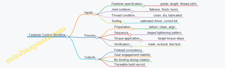
Step-by-Step Torque Procedure
-
Verify the fastener and joint match. Confirm thread pitch and length before touching a tool. A wrong pitch can feel “tight” early and still fail to clamp correctly.
-
Prepare threads and mating faces consistently. Remove burrs and chips. If you use lubricant or threadlocker, apply it the same way every time. For example, if you use a micro-drop on the screw threads, avoid smearing it onto the head face unless your procedure says to.
-
Use the correct driver and bit geometry. A worn bit rounds screw heads and increases friction variability. If the screw head starts to look polished or deformed, stop and replace the fastener or bit.
-
Tighten in a sequence that equalizes load. For multi-fastener covers, use a star pattern or alternating pairs. For single fasteners, tighten while holding alignment so the part doesn’t cock.
-
Apply torque in steps, not one hit. A two-step approach reduces overshoot. Example: tighten to 30% of target torque, then to 70%, then to final torque. This helps the joint seat and reduces scatter from thread settling.
-
Recheck torque after seating. After the final step, wait a short moment for material relaxation and then recheck the same fasteners to the final torque. On small joints, this catches cases where the first tightening step pulled the parts into alignment.
-
Perform a functional check immediately. Rotate the assembly by hand. You’re not testing performance yet; you’re checking for binding caused by uneven clamping or misalignment.
Torque Targets and Calibration Practices
Torque targets should come from your design intent and joint friction assumptions, but your procedure must also include calibration habits. Use a torque driver with a known calibration interval and document it in the build record.
A useful example for repeatability: if your target torque is 0.8 N·m, set your driver to 0.8 N·m for the final step, but still perform the staged tightening. If you skip stages, you’ll often see higher variation in the final seating state.
Common Failure Modes and How Torque Helps You Catch Them
- Thread galling or damage: Symptoms include gritty feel and rapid torque rise. Stop immediately; damaged threads change friction and can permanently alter preload.
- Uneven clamping from debris: A single chip under a head can tilt the joint. Consistent cleaning and a quick visual inspection prevent this.
- Over-torque causing distortion: Small parts can warp at modest torque. If hand rotation becomes stiff after tightening, reduce torque in the next build iteration and re-evaluate seating and surface prep.
Example: Tightening a Small Gearbox Cover
Assume a cover held by four M2 screws. Clean the cover and housing faces, then place the cover aligned. Tighten screws in an alternating pattern: 30% target on all four, then 70% target on all four, then final torque on all four. After the final pass, recheck each screw once. Finally, rotate the output shaft by hand; it should move smoothly with no sudden resistance.
Build Records That Actually Help
Record the fastener part number, torque driver ID, torque setting steps, and whether threads were dry or lubricated. Add a short note if you observed unusual feel or required bit replacement. This turns “it worked last time” into a traceable process you can reproduce.
7.3 Use Alignment Tools and Jigs to Reduce Assembly Error
Miniature harmonic drives punish sloppy alignment because small angular errors turn into large changes in tooth engagement and bearing loading. The goal of alignment tools and jigs is simple: control where parts sit, how they are centered, and how they are held while you torque, seat, and verify.
Foundational Idea: Define What “Aligned” Means
Start by listing the interfaces that must share a common axis or controlled offset. For a typical harmonic drive assembly, that usually includes the wave generator axis, the flexspline center, and the circular spline/bearing seats. A practical best practice is to translate each interface into one measurable constraint:
- Concentricity between bearing seats and the gear axis.
- Perpendicularity of shoulders that locate the wave generator.
- Axial position of the flexspline relative to the circular spline.
- Angular orientation if any features require indexing.
Example: if your circular spline seat is off-center by 20 µm, the flexspline will see a varying mesh depth around rotation. You may still get smooth motion during a quick hand test, but torque ripple and uneven wear show up later.
Jig Strategy: Constrain the Part Before You Constrain the Fastener
A common assembly mistake is tightening bolts to “pull” parts into place. In miniature builds, that can bend thin components or shift seats by tiny amounts that are hard to see. Instead, use a jig to establish alignment first, then torque.
A good jig workflow has three stages:
- Locate: place the part against a hard reference surface.
- Center: use a pilot feature or precision bushing to control radial position.
- Clamp: hold the stack rigidly while you fasten.
Alignment Tools That Actually Help
Use tools that match the error mode you’re trying to prevent.
- Centering pilots and bushings: A turned pilot that fits the bearing bore with a controlled clearance can center the wave generator or flexspline during assembly. Keep the pilot length short enough to avoid wobble, but long enough to guide.
- Reference shoulders and datum faces: Machine one face and one bore as the assembly datum. Then build the jig so every other part references those datums.
- Dial indicator fixtures: Before final torque, measure runout of the rotating element. If runout exceeds your threshold, stop and correct alignment rather than forcing it.
- Torque-limiting drivers with a repeatable sequence: For small screws, a consistent tightening order prevents uneven seating that looks like “mystery backlash.”
Systematic Assembly Procedure Using Jigs
Follow a repeatable sequence that reduces the number of times you handle parts.
- Dry fit and clean: Remove chips, burrs, and lubricant residue from mating seats. Even a thin smear can change seating height.
- Set the datum in the jig: Place the base component against the jig’s reference face and insert the centering pilot into the relevant bore.
- Stack alignment parts: Position the next component using the same pilot or a second centering bushing. If you use two pilots, ensure they share the same axis in the jig.
- Verify before torque: Use a dial indicator to check radial runout at a consistent radius. Record the value; it becomes your baseline for later builds.
- Torque while held: Clamp the stack in the jig and tighten using the specified sequence. Avoid “final tightening” after removing the clamp.
- Post-torque checks: Re-measure runout and confirm smooth rotation by feel and by a simple torque test if available.
Example: Suppose your pre-torque runout is 8 µm and post-torque becomes 25 µm. That pattern usually indicates uneven seating from fastener sequence or a clamp that allows micro-shift. Fix the sequence or add a locating feature rather than changing lubricant or preload.
Mind Map: Alignment Tools and Jig Logic
Example: A Simple Jig That Reduces Error
Build a “pilot-and-shoulder” jig for the wave generator seating operation.
- The jig base has a machined datum face.
- A precision pilot fits the wave generator bore.
- A clamp ring holds the assembly while you torque the screws.
During assembly, you can check runout at the flexspline outer diameter before torque. If runout is acceptable, you proceed; if not, you adjust the stack while the pilot is still guiding the part.
Practical Acceptance Thresholds
Set thresholds based on your design intent and measurement capability. A useful approach is to define two limits:
- Runout limit before torque to catch obvious mis-centering.
- Runout delta limit to catch seating shift caused by fastening.
Example: If your pre-torque runout is consistently under 10 µm but your post-torque delta varies widely, the issue is likely fastener sequence or clamp stiffness, not part-to-part variation.
Common Pitfalls to Avoid
- Forcing alignment with torque: it hides the real problem and can distort thin features.
- Using the wrong reference: if the jig references a non-datum surface, you measure the wrong thing.
- Skipping the pre-torque check: once bolts are torqued, correcting alignment becomes guesswork.
- Letting the jig flex: a clamp that bends under load can create alignment during measurement but not during torque.
When alignment tools and jigs are used this way, assembly becomes a controlled process rather than a careful guessing game. The payoff is not just smoother motion; it’s consistent engagement and predictable backlash across builds.
7.4 Confirm Gear Engagement and Smooth Rotation by Procedure
A harmonic drive can be mechanically correct yet still feel wrong during rotation. The goal of this procedure is to confirm engagement quality and smoothness using repeatable checks that isolate the cause when something is off. You will verify three things in order: (1) the wave generator actually drives the flexspline, (2) the circular spline teeth are meshing without binding, and (3) the assembly rotates smoothly across the full travel range.
Engagement Confirmation Workflow
Start with a clean, dry assembly stage unless your design requires a specific lubricant for assembly. Any grit acts like a tiny wedge, and the symptoms look like misalignment.
-
Establish a reference rotation Mark the wave generator position relative to the housing and choose a rotation direction. Then rotate slowly by hand through the expected operating range. Smoothness should be consistent, not “smooth in one quadrant and sticky in another.”
-
Check for consistent resistance During slow rotation, resistance should rise and fall gradually. A sharp spike usually indicates a localized interference: a tooth edge contacting where it should not, a burr, or a seat that is slightly tilted.
-
Verify engagement by feel and geometry With the assembly held steady, rotate in small increments (for example, 10–15 degrees at a time). After each increment, pause and observe whether the mechanism “settles” back or stays where you left it. A mechanism that repeatedly relaxes can be experiencing uneven tooth contact.
-
Confirm full-cycle smoothness Repeat the rotation through the entire range. Smoothness should not degrade near the ends unless your design includes intentional end-stop behavior. If the ends are worse, suspect preload, bearing seating, or housing interference.
-
Record the symptom pattern Note where the problem occurs: at the same angular positions every time, or randomly. Repeatability points to geometry or alignment; randomness points to debris, lubrication mismatch, or assembly handling.
Practical Mind Map
Mind Map: Gear Engagement and Smooth Rotation Procedure
Example: A Smoothness Check That Actually Tells You Something
Imagine you rotate the assembly by hand and feel a noticeable spike every time you reach the same angular position. You repeat the cycle three times and the spike lands at the same mark. That pattern strongly suggests a localized interference rather than debris.
Next, you disassemble only to the level needed to inspect the most likely contact surfaces. Look for a burr on tooth edges, a raised machining mark on a seat, or a slight tilt from an imperfect seating surface. If you find a burr, remove it carefully and reassemble with the same preload setting. Then repeat the incremental rotation with pauses. If the spike disappears and the resistance profile becomes gradual, you have confirmed engagement quality.
Example: End-Range Stickiness
If rotation is smooth in the middle but becomes sticky near both ends of travel, the issue often relates to how preload and bearing seating behave under the load path. Reduce preload to the next allowable setting within specification, then repeat the full-cycle smoothness check. If the end stickiness reduces proportionally, you have identified preload as the dominant contributor.
Procedure Output Criteria
You should be able to state, for your specific build, that engagement is confirmed when:
- Resistance changes are gradual with no sharp spikes.
- Incremental pauses do not show repeated settling behavior.
- Smoothness is consistent across the full rotation range.
- The symptom pattern is either absent or repeatable with a known, addressed cause.
This procedure turns “it feels off” into a structured observation you can act on, without guessing whether the problem is engagement, alignment, preload, or cleanliness.
7.5 Document Assembly Settings for Repeatable Builds
Repeatable harmonic drive and precision servo assemblies start with one unglamorous habit: recording the exact settings that affect geometry, preload, and alignment. If you only log “assembled” or “torqued,” you’ll eventually rediscover the same problem with different numbers. The goal here is to capture settings in a way that lets a second builder reproduce the first build without guessing.
What to Record and Why
Document three categories of information: (1) the physical state of parts, (2) the assembly actions that change that state, and (3) the measurements that confirm the result.
-
Part state includes serial numbers, batch IDs, and any measured dimensions that influence fit. For example, record the flexspline thickness measurement taken before machining or finishing. If you later see a control loop that behaves differently, you can correlate it to a thickness shift rather than blaming the controller.
-
Assembly actions include preload method, torque values, alignment steps, and any controlled offsets. For small fasteners, record the torque tool model and calibration date. If you used a torque-to-angle method, record the angle and the starting torque.
-
Verification measurements include runout, engagement feel checks, backlash readings, and sensor zero references. A simple example: after assembly, rotate the output shaft by hand and record the number of degrees from a defined reference until motion becomes smooth. That “smoothness threshold” becomes a repeatability indicator when you compare builds.
A Practical Settings Template
Use a single-page form that can be filled during assembly. Keep it structured so the same fields appear every time.
- Build identifiers: project ID, date, operator, fixture ID.
- Component traceability: motor serial, wave generator serial, flexspline serial, circular spline serial, bearings serial.
- Measured inputs: key dimensions (e.g., flexspline thickness, bearing seat diameter, shaft diameter), surface finish notes if relevant.
- Assembly parameters: preload setting method, preload value or target deflection, torque values, torque sequence, alignment jig used, any shimming thickness.
- Verification results: backlash at a defined torque, runout at a defined radius, sensor zero offset, friction check result.
Example: if you preload by tightening a clamp until a dial indicator reads a target deflection, record the deflection reading, the dial indicator model, and the measurement location. That’s the difference between “tightened” and “reproduced.”
Mind Map: Assembly Settings Documentation
Defining References So Numbers Mean Something
Most assembly documentation fails because measurements aren’t tied to a reference. Fix this by defining where the measurement starts and ends.
- Backlash reference: specify the direction of approach (clockwise to counterclockwise, for instance), the preload torque used during the check, and the angular resolution of the measurement tool.
- Runout reference: specify the datum surface and the radius where runout is measured. Measuring at a different radius changes the number even when the part is identical.
- Sensor zero reference: specify the mechanical position used for zeroing and the method used to set it (software offset, physical index mark, or calibration routine).
A concrete example: if you set sensor zero with the wave generator at a particular clocking angle, record that angle relative to a marked feature. Otherwise, the same “zero” can correspond to different internal gear engagement states.
Recording Calibration and Tooling Details
Small assemblies are sensitive to tool behavior. Record the torque tool ID, calibration date, and whether you used a new bit or a worn one. If you use a dial indicator or height gauge, record the model and the measurement range used.
If you need a date, use a consistent format and keep it in the template. For example, “Calibration date: 2026-02-20” is more useful than “calibrated recently.”
Example: Two Builds with One Changed Setting
Build A: preload set to target deflection of 0.120 mm at the specified dial indicator location; torque sequence followed as T1 then T2; backlash measured at 0.8 N·m approach torque equals 0.9 arc-min.
Build B: same parts and same sequence, but preload deflection recorded as 0.112 mm. Backlash measured equals 1.4 arc-min and the position loop shows a slightly larger steady-state error under the same motion profile.
The point isn’t that the preload “caused” everything; it’s that the documentation makes the relationship testable. When you compare builds, you can focus on the one parameter that actually changed.
Final Checklist for Repeatability
Before closing the build record, confirm that every field has either a value or an explicit “not applicable.” If a measurement wasn’t taken, record why and what you used instead. Repeatable builds are built from complete records, not from hope.
8. Precision Servo Calibration and Tuning Workflows
8.1 Calibrate Sensor Scaling and Zero References
A servo can be perfectly tuned in software and still behave badly if the sensor’s numbers do not match the mechanism’s real angles or positions. Calibration fixes two things: scaling (how many units per physical unit) and zero reference (what physical position corresponds to sensor reading 0). Treat them as separate problems so you can debug them without guessing.
Foundations: What “Scaling” and “Zero” Mean
Scaling answers: “If the shaft rotates 10°, what sensor change should I expect?” For an encoder, scaling is often counts per revolution divided by gear ratio; for a resolver or potentiometer, it’s volts or digital counts per mechanical angle.
Zero reference answers: “When the mechanism is at a known reference position, what sensor reading should I record as zero?” For harmonic drives, this is especially important because the flexspline strain and assembly preload can shift the effective neutral point.
A practical rule: calibrate zero first using a repeatable mechanical reference, then compute scaling using multiple measured positions. If you do scaling first, you may bake a wrong zero into every later calculation.
Mind Map: Sensor Calibration Workflow
Step 1: Establish a Repeatable Mechanical Reference
Pick a reference that you can hit the same way every time. Common choices are a hard stop, a fixture index pin, or a marked alignment surface. For a hard stop, ensure the stop is rigid enough that the mechanism doesn’t “settle” differently between runs. If the stop is compliant, you’ll measure compliance as if it were sensor error.
Example: You mount the servo in a fixture with a dowel pin that engages a notch on the output housing. You then rotate the output until it seats against the pin. That seating position becomes your reference.
Step 2: Capture Zero Reference Carefully
Move to the reference position, then record the sensor reading. For incremental encoders, you typically compute an offset from the current count. For absolute encoders, you store the raw angle value at the reference.
Best practice: average multiple samples while holding the mechanism still. Even if the sensor is stable, the mechanism may micro-vibrate as the motor controller applies holding torque. Averaging reduces the influence of that tiny motion.
Example: At the reference, take 100 samples over 0.5 seconds, compute the mean, and store it as zero_offset. Also record the standard deviation; if it’s large, your reference is not repeatable or the mechanism is still moving.
Step 3: Compute Scaling Using Multiple Positions
Scaling is easiest when you assume a linear relationship between sensor units and physical angle over the calibration range. For most servo mechanisms, that’s accurate enough if you avoid backlash transitions during measurement.
Procedure:
- Choose at least 3–5 physical positions across the operating range.
- For each position, approach it from the same direction to reduce backlash effects.
- Record sensor readings and compute physical angle from your reference geometry.
- Fit a line:
physical_angle = scale * (sensor - zero_offset).
Example with an incremental encoder:
- Encoder resolution: 4096 counts/rev (motor shaft)
- Gear ratio: 50:1 (motor:output)
- Expected counts per output revolution: 4096 * 50 = 204,800 counts
- If your measured output rotation from reference to a second datum is 30°, you can compute scale from the sensor delta divided by 30°.
If your fitted line shows a noticeable curvature, it usually means you crossed a backlash boundary, the reference is shifting, or the gear mesh is not consistent during the measurement.
Step 4: Validate with Residual Error and Repeatability
Validation should be mechanical and numerical.
Numerical check: After applying scale and zero_offset, command several positions and compare measured physical angle against the expected values. Look at residual error, not just the average.
Mechanical check: Repeat the same move sequence multiple times. Repeatability errors often come from fixture looseness, gear settling, or inconsistent approach direction.
Example: Command 10°, 20°, 30° in the same direction each time. If the mean error is small but the spread grows, the issue is not scaling; it’s reference stability or approach control.
Step 5: Implement the Conversion Function
Keep the conversion explicit so you can log intermediate values during debugging.
physical_angle = scale * (sensor_units - zero_offset)

where:
- sensor_units is raw encoder counts or raw absolute angle
- zero_offset is sensor_units at the mechanical reference
- scale converts sensor units to degrees or radians
When you log, store sensor_units, sensor_units - zero_offset, and physical_angle. If the controller behaves oddly, you can see whether the problem is in the sensor conversion or later in the control loop.
Common Pitfalls and How to Avoid Them
- Zero captured while moving: If you record zero during motion, you’ll store a moving target.
- Scaling computed across backlash: Approach each calibration point from the same direction.
- Mixing motor and output angles: Always state whether your calibration maps to motor shaft angle or output shaft angle.
- Reference that “creeps”: If the mechanism relaxes after seating, wait for settling before sampling.
A good calibration ends with numbers you can trust: a stored zero_offset, a scale factor derived from multiple points, and a validation report showing small residual error and tight repeatability.
8.2 Characterize Friction and Backlash Effects on Control
Friction and backlash are the two gremlins that make a servo look “almost” right. Friction mainly distorts the relationship between commanded torque and achieved motion, while backlash creates a dead zone where small commands do nothing until the mechanism takes up slack. Characterizing both lets you separate control problems from mechanical problems, and it prevents tuning from compensating for the wrong thing.
Foundational Concepts for Measurement
Start by defining what you can measure. For a precision servo, you typically have at least position (from an encoder or resolver) and motor current (from a current loop). If you also have torque estimation or a load cell, even better. Backlash is best observed in the position domain as hysteresis between increasing and decreasing motion. Friction is best observed as a torque offset that depends on direction and speed.
A practical mental model:
- Backlash: a gap in the kinematic chain, producing different position outcomes for the same input depending on whether you approached from the positive or negative direction.
- Friction: a resistive torque that changes with speed and direction, often with a stiction component near zero speed.
Mind Map: What to Measure and Why
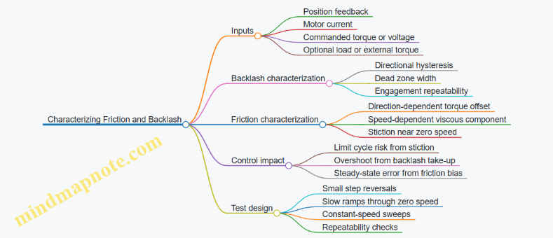
Backlash Characterization Workflow
Backlash shows up when you reverse direction. Use a sequence of small position reversals around a nominal angle, keeping the commanded motion small enough that you do not excite other nonlinearities like structural flex. A good starting point is a set of reversals with increasing amplitude: for example, ±5 arcseconds, ±10 arcseconds, ±20 arcseconds, and so on until you see consistent engagement.
For each reversal, record the measured position trajectory and compute the difference between the “approach from positive” and “approach from negative” curves. The dead zone width is the smallest commanded reversal that produces a clear change in measured motion. Repeat the same test several times without changing temperature or supply voltage, because backlash can shift slightly with preload seating.
A concrete example: suppose you command a sinusoid of small amplitude and measure that the output position lags on reversal by about 15 arcseconds before it starts moving. That 15 arcseconds is not a control parameter yet; it is a mechanical fact you can use to adjust how you handle direction changes. If your controller tries to correct error inside that dead zone, it will keep integrating until the slack is taken up, which can cause a step-like overshoot.
Friction Characterization Workflow
Friction is direction-dependent and speed-dependent. To separate components, run tests that isolate speed while minimizing backlash effects. One approach is to use a unidirectional constant-speed sweep first, then repeat in the opposite direction.
- Constant-speed sweep
- Command a series of steady velocities (or slow ramps that settle quickly).
- For each speed, estimate the required torque from motor current using your motor constants and any known gear ratio.
- Plot estimated torque versus speed for both directions.
You will usually see a roughly linear trend at moderate speeds (a viscous-like term) plus an offset that flips sign with direction. Near zero speed, the torque required to start motion is larger than the torque required to keep moving; that difference is stiction.
- Slow reversal through zero
- Command a small oscillation around zero velocity, but keep the amplitude small enough that backlash is either already characterized or not dominant.
- Measure the torque/current needed to initiate motion each time you reverse.
If you observe that the current jumps at reversal and then decays as speed builds, that is a sign of stiction. If instead the current changes smoothly with no jump, stiction may be small and friction is mostly viscous.
Turning Measurements into Control-Relevant Parameters
Once you have backlash width and friction behavior, you can map them to control consequences.
- Backlash width informs how aggressively you should correct during direction changes. A controller that assumes a continuous plant will “fight the gap.” A practical mitigation is to reduce integral action around reversals or to gate integration when measured error is within the dead zone.
- Friction bias informs steady-state error. If friction adds a direction-dependent torque offset, a proportional-only controller will leave a residual error that changes sign with direction. Integral action can remove it, but if backlash is present, integral can accumulate during the dead zone and then release abruptly.
A simple diagnostic: run the same position command in both directions at the same speed. If the steady-state error magnitude is similar but the sign flips, friction bias is likely. If the error is asymmetric only around reversals and shows a threshold behavior, backlash is likely.
Example Test Plan for a Miniature Harmonic Drive Servo
- Step 1: Backlash reversals
- Command position reversals of increasing amplitude around a fixed angle.
- Record output position and determine dead zone width.
- Step 2: Unidirectional speed sweep
- Command constant velocities in the positive direction across a small speed range.
- Record current and estimate torque versus speed.
- Step 3: Opposite direction sweep
- Repeat Step 2 in the negative direction.
- Step 4: Slow reversal through zero
- Command a small oscillation that crosses zero velocity.
- Identify stiction behavior and any current spikes.
Finally, validate by running a closed-loop motion profile that includes both steady segments and reversals. If the output shows step-like jumps at reversals, backlash handling is insufficient. If it shows a consistent offset during steady motion, friction bias compensation is insufficient. When both are addressed, the controller stops “chasing ghosts” and starts behaving like a predictable system rather than a guess-and-check machine.
8.3 Tune Position and Velocity Loops With Measured Data
A good tuning workflow starts with measurements that explain what the system is doing, not what you wish it were doing. For a precision servo, you typically have two coupled loops: a velocity loop that shapes how fast the motor moves, and a position loop that decides where it should be. The key is to tune velocity first, then position, using the same measurement signals you will later rely on for validation.
Step 1: Prepare Signals and Define What “Good” Means
Measure at least these signals during controlled tests: commanded position, measured position, commanded velocity (or the velocity controller output), measured velocity, motor current (or torque proxy), and supply voltage if available. If you only have position and current, you can still tune, but you must treat velocity estimates as part of the system you are tuning.
Define acceptance criteria in measurable terms. For example: overshoot less than 5% on a step, settling within 2% of final value in under 150 ms, and steady-state position error under a small threshold at a constant load. For velocity, define peak tracking error and how quickly the loop returns to steady state after a disturbance.
Step 2: Tune the Velocity Loop Using Small, Safe Excitations
Velocity tuning should be done with position held constant or with a slow position ramp so the position loop does not interfere. Use a small velocity step or a short trapezoid velocity command. Keep the amplitude low enough to avoid saturating current limits.
From the measured response, extract three practical quantities:
- Delay: the time between the command change and the first noticeable change in measured velocity.
- Damping: whether the response overshoots and oscillates.
- Bandwidth: the frequency range where tracking error stays small.
A simple way to reason about loop behavior is to treat the velocity loop as a second-order system with delay. If you see oscillation, reduce loop gain or increase filtering. If you see sluggish tracking, increase loop gain or reduce excessive filtering.
Step 3: Use Error Signals to Choose Adjustments
Compute velocity error as \(e_v = v_{cmd} - v_{meas}\). Then compute current or torque command error if you have it. When you adjust gains, watch which error shrinks and which grows.
- If velocity error decreases but current spikes, you are likely pushing too hard into friction or backlash effects.
- If velocity error stays high and current is steady, the loop may be underpowered or filtered too aggressively.
- If velocity error oscillates in sign, you likely have too much gain relative to delay.
This is where measured data beats intuition. A controller that looks stable in simulation can still misbehave if your measured delay is larger than expected.
Step 4: Tune the Position Loop After Velocity Is Stable
Once velocity tracking is crisp, position tuning becomes mostly about shaping how the system responds to position commands without exciting oscillations.
Start with position proportional gain only, then add integral carefully. Integral helps remove steady-state error from constant disturbances like gravity on a gimbal, but it can also increase overshoot if the velocity loop is not well damped.
Use a position step test with a known load condition. Record overshoot, settling time, and the shape of the error curve. A useful diagnostic is to compare position error and velocity command: if position error changes sign while velocity command still ramps strongly, you are likely overshooting due to integral action or insufficient damping.
Step 5: Validate with Disturbance and Motion Profiles
Validation should include more than one test. Use:
- A step to check transient behavior.
- A slow ramp to check steady-state tracking.
- A short disturbance by applying a brief external torque or load change.
If you see a velocity tracking dip during the disturbance but position recovers quickly, your velocity loop is doing its job. If position lags and current saturates, you may need to revisit velocity gains or reduce position aggressiveness.
Mind Map: Position and Velocity Tuning with Measured Data
Example: Interpreting a Velocity Step Test
Suppose a 0.5 rad/s velocity step produces measured velocity that rises slowly, then overshoots by 12%, and oscillates twice before settling. The likely story is: delay is nontrivial and damping is insufficient. Reduce velocity loop gain slightly and reduce filtering delay (or increase damping via controller structure). After changes, repeat the same step and compare overshoot and settling time.
Example: Position Tuning with Integral
After velocity tuning, you add integral to remove steady-state error under a constant load. You run a position step and observe 8% overshoot and longer settling than before. The measured position error crosses zero early, but the velocity command remains elevated longer than expected. Reduce integral gain or increase the integral anti-windup effectiveness so the controller does not keep integrating while the actuator is effectively constrained.
Example: Disturbance Rejection Check
During a constant-position hold, apply a brief torque disturbance. If current spikes and velocity deviates, the velocity loop is reacting. If position error grows and takes a long time to return, the position loop may be too aggressive or integral may be too strong. Adjust position gains while keeping the velocity loop unchanged, then re-test the same disturbance.
When you tune this way, each gain change has a measurable cause-and-effect chain: you excite the system, observe error shapes, and adjust the smallest set of parameters that corrects the observed behavior. That’s the whole trick—boring on purpose, accurate by design.
8.4 Validate Control Performance Under Load and Motion Profiles
Validation under load is where “it tracks nicely on the bench” becomes “it tracks when the mechanism is actually doing work.” The goal is to confirm that your position and velocity loops behave predictably across the motion shapes and torque demands your drone or robot will see.
Start with What “Performance” Means
Define measurable outcomes before you run tests. For each axis or actuator, pick:
- Tracking error: peak and RMS position error over a motion segment.
- Steady-state error: final error after settling.
- Dynamic behavior: overshoot, settling time, and oscillation amplitude.
- Control effort: motor current or commanded torque magnitude.
- Robustness: sensitivity to load changes and friction variation.
A practical example: if your servo drives a robotic link, you might accept a small overshoot during fast moves but require near-zero steady-state error when the link stops.
Build a Load-Realistic Test Matrix
Use a small set of motion profiles and load cases that cover the important dynamics.
Load cases should include:
- No external load (baseline).
- Nominal load (the expected operating torque).
- High load (near your actuator’s comfortable limit).
- Direction reversal (same magnitude load, opposite direction), because friction and backlash effects often differ.
Motion profiles should include:
- Step or short move to expose overshoot and settling.
- Trapezoidal velocity to test acceleration and deceleration behavior.
- Sine or chirp-like motion to reveal frequency-dependent tracking issues.
Keep the matrix small but intentional. If you test only one profile at one load, you’ll learn less than you think.
Instrumentation That Actually Helps
Measure signals that let you separate “control problem” from “mechanical problem.” At minimum:
- Commanded position/velocity and measured position.
- Motor current (or estimated torque) and supply voltage if available.
- Temperature or at least a proxy like motor case temperature.
- If possible, a friction proxy such as current asymmetry between directions.
Concrete example: if tracking error grows mainly when current saturates, the issue is likely actuator torque limits or current-loop bandwidth, not the position loop gains.
Validate with a Stepwise Procedure
- Confirm loop stability at the baseline load using your existing tuning. You’re looking for consistent settling and no sustained oscillation.
- Increase load gradually while repeating the same motion profile. Watch for changes in overshoot and settling time.
- Repeat at the same load but with different motion shapes. If a controller tracks trapezoids but fails on sine motion, your bandwidth or filtering choices may be mismatched.
- Test reversal moves. Compare error and current waveforms for positive-to-negative and negative-to-positive transitions.
A useful rule of thumb: if the error pattern scales with load magnitude, your controller is likely coping with the plant. If the error pattern changes shape, you may be hitting nonlinearities like friction, gear engagement effects, or sensor quantization.
Interpret Results Using a Cause Map
When performance is off, don’t guess randomly. Use a structured interpretation.
Mind Map: Load and Motion Validation Logic
Example: Trapezoidal Move Under High Load
Suppose a servo tracks a trapezoidal velocity command at nominal load with small overshoot. Under high load, you observe:
- Position overshoot increases.
- Settling time doubles.
- Current peaks flatten at a limit.
Interpretation: the controller is demanding more torque than the actuator can provide, reducing effective damping during deceleration. A targeted fix is to adjust the motion profile limits (reduce acceleration/jerk) or retune gains to avoid driving the current loop into saturation during transients.
Example: Sine Motion Shows Frequency-Dependent Error
Now keep load constant and switch to a sine position command. If tracking error is small at low frequency but grows sharply near a specific band, you likely have a bandwidth mismatch or unmodeled dynamics (for instance, compliance in the transmission or sensor filtering delay). The evidence is in the phase lag and the error waveform repeating at the command frequency.
Document What You Learned
For each test, record:
- Motion profile parameters (amplitude, duration, acceleration).
- Load condition description and how it was applied.
- Metrics (peak/RMS error, overshoot, settling time).
- Waveform notes (current saturation, asymmetry on reversal).
This turns validation from “we ran some tests” into a repeatable decision process for tuning and integration.
8.5 Record Calibration Results for Reproducible Production
Reproducible production starts with treating calibration as a measurable artifact, not a one-time event. The goal is simple: when you repeat the same build process, the servo should behave the same way within defined tolerances, even if assembly happens on different days or by different people.
What to Record So Results Can Be Recreated
Record calibration outputs in three layers: setup facts, measured behavior, and applied parameters.
-
Setup facts capture “what the system looked like” during calibration. Include firmware version, controller gains state, sensor wiring polarity, motor phase mapping method, encoder resolution settings, and any gear backlash compensation mode. Also log ambient conditions if they affect your measurements, such as enclosure temperature and whether the actuator was allowed to thermally settle.
-
Measured behavior captures “what the system did.” Store raw or minimally processed traces for position error, velocity error, and torque/current command during representative motion profiles. Include backlash characterization results such as deadband width and the direction dependence of friction.
-
Applied parameters capture “what you changed.” Save the final controller parameters, scaling factors, feedforward terms, friction model coefficients (if used), and any limits or filters. If you used a friction estimate derived from a specific test, store the test conditions so the estimate can be interpreted later.
A practical example: if your position loop uses a velocity feedforward term, record the exact feedforward gain and the velocity units used. Otherwise, the same numeric gain can mean different physical behavior after a scaling change.
How to Structure Calibration Records
Use a consistent record template so engineers and technicians can find the same information every time.
- Header: build ID, actuator serial, motor type, gear ratio, sensor model, controller hardware ID, and calibration date (for example, 2026-02-20).
- Inputs: calibration procedure version, motion profile definition, sample rate, filtering settings, and any safety limits.
- Outputs: measured metrics (overshoot, settling time, steady-state error, repeatability), plus the raw traces used to compute them.
- Parameters: final gain set, scaling constants, compensation settings, and any lookup tables.
- Acceptance: pass/fail criteria and which tests were used to decide.
If you only store “final gains,” you’ll eventually face a mystery when a unit behaves differently. When you store the measured traces and the exact motion profile, you can compare behavior rather than guessing.
Mind Map: Calibration Records for Reproducible Production
Examples of Record Entries That Prevent Common Failures
Example 1: Scaling mismatch
- Record: encoder counts per revolution, any gear ratio applied in software, and the unit conversion used for velocity.
- Why it matters: if one build uses counts-per-rev directly and another uses a pre-scaled value, the same gain produces different motion.
Example 2: Backlash compensation inconsistency
- Record: backlash compensation mode, deadband width, and whether compensation is applied on the approach direction only.
- Why it matters: backlash is not symmetric in many small mechanisms, so “one number” rarely describes it fully.
Example 3: Filter settings drift
- Record: sensor filtering cutoff frequency and any digital smoothing window length.
- Why it matters: filtering changes phase lag, which shifts stability margins and alters overshoot.
A Simple Workflow That Keeps Records Honest
- Calibrate once per procedure version and store the full record template.
- Run a short verification test on every unit using the same motion profile and log the same metrics.
- Compare metrics to the acceptance band derived from earlier calibration records.
- If a unit fails, store the failure traces and the exact parameter set used, so the next investigation has evidence.
Acceptance Metrics to Store
Store metrics that connect directly to production decisions:
- Steady-state error at a fixed position target after settling.
- Repeatability measured as the spread of final position across repeated cycles.
- Backlash behavior measured as deadband width and the difference between approach directions.
- Dynamic quality measured as overshoot and settling time under the same motion profile.
When these metrics are recorded consistently, you can spot whether a change came from assembly variation (measured behavior shifts) or from parameter changes (applied parameters differ).
Final Checklist for Reproducible Records
- Every record includes setup facts, measured behavior, and applied parameters.
- Every record references the procedure version and the motion profile definition.
- Every record includes pass/fail criteria and the traces used to decide.
- Every record is tied to a build ID so you can reproduce the exact configuration later.
Do this, and calibration becomes a repeatable manufacturing step rather than a memory test. Your future self will thank you, mostly by not making you re-run the same measurements twice.
9. Managing Thermal Effects and Material Behavior
9.1 Identify Thermal Sources in Small Actuation Systems
Small harmonic drives and precision servos turn electrical power into heat through a few repeatable paths. The trick is to identify which path dominates in your specific build, because the same component can be “cool” in one duty cycle and “warm” in another.
Start with a Thermal Budget Mindset
Begin by listing every place where power becomes heat. In a compact actuator, the heat sources usually include motor copper loss, motor iron loss, bearing friction, gear mesh friction, flexspline strain hysteresis, seal drag, and any electrical losses in drivers and wiring. Then map each source to a thermal path: conduction into the housing, conduction into the shaft and bearings, convection to air, and radiation from exposed surfaces. If you can’t measure temperatures yet, you can still estimate relative dominance by comparing how each loss scales with current, speed, and torque.
Motor Losses That Show Up First
Motor copper loss is proportional to current squared. When you command higher torque, the current rises and heat follows quickly. Motor iron loss depends on electrical frequency and flux; it becomes more noticeable at higher speeds even when torque is modest. A practical check is to run the actuator at constant speed with low torque and then at the same speed with higher torque. If temperature rises mainly in the high-torque case, copper loss is likely the main contributor.
Bearing and Seal Friction
Bearings convert a portion of rotational energy into heat through lubricant shear and rolling contact losses. Seal drag adds heat that often scales with differential pressure and sliding speed. In small assemblies, seals can be a surprise: a thin lip seal that seems “light” can still create meaningful drag at high rpm. A simple example: compare temperature rise during free rotation (no load) versus loaded rotation at the same speed. If the loaded case adds only a little extra heat, friction sources that exist even without load—like seals and bearings—are probably already doing most of the work.
Gear Mesh and Flexspline Hysteresis
In a harmonic drive, the flexspline experiences cyclic strain as it engages the wave generator and circular spline. That cyclic deformation produces hysteresis loss, which can be significant even when backlash is controlled well. Gear mesh friction adds additional heat, especially if lubrication is marginal or if surface finish causes higher micro-slip. A useful diagnostic is to vary lubrication condition while keeping torque and speed constant. If temperature rise changes noticeably, friction and boundary lubrication effects are likely involved.
Electrical Driver and Wiring Losses
Driver electronics generate heat through switching losses, conduction losses in power stages, and inefficiencies in current regulation. Wiring resistance also contributes copper loss, particularly if long leads or thin conductors are used. To separate actuator heat from driver heat, measure temperatures at both the motor housing and the driver enclosure during the same run. If the driver temperature rises faster than the motor, you may be chasing the wrong source.
Thermal Path Bottlenecks
Even if you know the heat sources, you still need to know where heat goes. Small parts often have limited conduction area, so a modest loss can create a large temperature rise if the thermal path is poor. Look for interfaces with high contact resistance: press fits without proper surface prep, anodized layers under clamping surfaces, or misaligned housings that reduce contact area. A practical example: two housings with the same geometry can differ in temperature rise if one has better metal-to-metal contact at the bearing seat.
Mind Map: Thermal Sources and How to Spot Them
A Systematic Identification Workflow
- Instrument the obvious places: motor housing, bearing region if accessible, and driver enclosure.
- Run two controlled baselines: constant speed low torque, then constant speed higher torque.
- Add a mechanical baseline: compare no-load and loaded at the same speed.
- Change one variable at a time: lubrication condition or seal configuration, not both.
- Interpret temperature rise rates: faster rise with current points to copper loss; faster rise with speed points to iron loss and friction.
Example: Interpreting a Confusing Temperature Pattern
Suppose motor housing temperature rises sharply with torque, but driver temperature stays nearly flat. That pattern points to motor copper loss and/or load-dependent mechanical losses like mesh friction. Now repeat with a different seal that reduces drag. If the no-load temperature drops while the loaded temperature changes less, seal drag is a major contributor to baseline heating, while load-dependent losses still dominate under torque.
By the end of this process, you should be able to name the top one or two thermal sources and the main thermal bottleneck, which sets up the next step: choosing mitigation actions that actually address the dominant heat path.
9.2 Account for Expansion in Gear Mesh and Bearing Fits
When temperature changes, metal parts do not politely stay the same size. In a harmonic drive, the flexspline, circular spline, wave generator, and bearings all expand at different rates and in different directions. The result can be a tighter mesh, a looser mesh, or a fit that shifts from “smooth assembly” to “mysterious binding.” The goal is to predict where expansion matters and design clear allowances so the mechanism behaves consistently across the expected temperature range.
Foundational Concepts That Control Fit Changes
Start with linear thermal expansion:
- A part’s length changes by \(\Delta L = \alpha L \Delta T\), where \(\alpha\) is the coefficient of thermal expansion, \(L\) is the relevant dimension, and \(\Delta T\) is the temperature change.
- For diameters, use the same idea: \(\Delta D \approx \alpha D \Delta T\). A small diameter change can matter a lot when you are working with press fits, bearing seats, or thin gear features.
Next, remember that gear mesh clearance and bearing fit are not single numbers. They are outcomes of multiple dimensions that each expand differently. A bearing inner ring may grow relative to a shaft, while the outer ring grows relative to a housing. Meanwhile, the flexspline tooth engagement depends on both radial and circumferential geometry.
Where Expansion Shows Up in Harmonic Drives
Gear mesh behavior is sensitive to:
- Radial growth of the circular spline and flexspline.
- Axial growth that can shift engagement depth if thrust faces are constrained.
- Wave generator geometry that changes the effective strain distribution.
Bearing behavior is sensitive to:
- Inner ring-to-shaft fit changes that affect preload and friction.
- Outer ring-to-housing fit changes that affect creep, micro-slip, and alignment.
- Housing and shaft materials that may have different \(\alpha\), creating differential expansion.
A practical way to think about it: if thermal expansion reduces clearance where you need clearance, you get higher friction and possible tooth interference. If it increases clearance where you need stiffness, you get more compliance and control sensitivity.
Systematic Fit Allowance Method
- Define the temperature delta \(\Delta T\) between assembly and the operating condition. If assembly happens at a controlled shop temperature, use that as the baseline.
- List critical dimensions: bearing seat diameter, shaft diameter, gear mesh radial clearance contributors, and any locating features that constrain axial position.
- Compute expected diameter changes for each part using \(\Delta D = \alpha D \Delta T\).
- Convert fit logic into clearance logic. For example, if you have a press fit at assembly, you want to know whether it becomes tighter or looser at temperature.
- Check worst-case stack-ups. Use the largest plausible dimension for one part and the smallest for the mating part when assessing minimum clearance, and reverse for maximum clearance.
Mind Map: Expansion Effects and Fit Control
Concrete Example: Bearing Fit and Mesh Clearance
Assume a steel shaft and an aluminum housing. The shaft seat diameter is 10.00 mm, the housing bore is 20.00 mm, and the temperature rise is 40°C. Using typical coefficients (steel \(\alpha\) ≈ 12×10⁻⁶/°C, aluminum \(\alpha\) ≈ 23×10⁻⁶/°C):
- Shaft diameter growth: \(\Delta D_s \approx 12\times10^{-6} \cdot 10.00 \cdot 40 \approx 0.0048\) mm.
- Housing bore growth: \(\Delta D_h \approx 23\times10^{-6} \cdot 20.00 \cdot 40 \approx 0.0184\) mm.
If the bearing outer ring relies on the housing bore for a snug fit, the housing expanding more than the outer ring can reduce interference, lowering friction but increasing the chance of micro-slip under load. Meanwhile, the shaft expansion can increase inner ring interference, raising friction and heat. In a harmonic drive, that heat can further change clearances, so the “fit at temperature” matters more than the “fit at assembly.”
Practical Checks That Prevent Surprises
- Measure fit behavior at temperature: after thermal soak, verify smooth rotation torque and any axial play that should remain stable.
- Inspect for tooth interference risk: if you see increased torque at higher temperature without corresponding load increase, suspect reduced mesh clearance.
- Use consistent material pairing: when possible, choose material combinations that keep differential expansion small for the most constrained interfaces.
A good design ends up with a mechanism that changes size, but not its functional relationships. The math tells you which relationships are at risk; the checks confirm whether the real assembly matches the model.
9.3 Control Lubrication Viscosity and Temperature Sensitivity
Lubrication viscosity is the “how easily the lubricant flows” parameter, and temperature sensitivity is the “how much that flow changes when things heat up.” In miniaturized harmonic drives and precision servos, small clearances mean the lubricant film thickness and shear behavior can change noticeably with even modest temperature swings. The goal is to control viscosity at the operating temperature, not just pick a lubricant that looks good on a datasheet.
Foundational Concepts That Drive Viscosity Control
Viscosity typically drops as temperature rises. That reduces viscous drag, but it can also thin the film, increasing metal-to-metal contact risk and changing friction torque. In a harmonic drive, friction torque affects control loop behavior because it changes the relationship between commanded motion and measured position. In a servo, viscosity also affects motor current demand indirectly by changing the load torque seen by the motor.
A practical way to reason about this is to separate three temperatures:
- Ambient: what the enclosure starts at.
- Bulk lubricant temperature: the average temperature of the oil/grease in the gear cavity.
- Local interface temperature: the hottest region at tooth contact, which can exceed bulk temperature during high load.
You can’t measure local interface temperature easily, so you design for bulk temperature and use friction and current as indirect indicators.
Mind Map: Viscosity and Temperature Sensitivity
Systematic Workflow from Selection to Validation
Choose a Lubricant with the Right Viscosity Window
Start by defining the expected bulk lubricant temperature range for the component. For example, if a gimbal servo runs in a drone bay that can warm from 20°C to 55°C, assume bulk lubricant might sit around 35–60°C depending on duty cycle. Then select a lubricant whose viscosity stays within a usable range across that interval.
A concrete example: if you choose a lubricant that is very viscous at 20°C, it may cause high starting friction. That can create a noticeable deadband in position control. If you choose one that becomes too thin at 60°C, you may see increased friction variation during repeated motion, which shows up as jitter or limit-cycle behavior.
Account for Grease Behavior Versus Oil Behavior
Grease is not just “thicker oil.” Its thickener can release oil under shear, and its effective viscosity can change with how the gear cycles. That means two tests with the same bulk temperature but different motion profiles can produce different friction.
Example: a harmonic drive that is mostly static with occasional bursts may “pump” lubricant differently than one that continuously cycles. The burst case can leave the interface under-lubricated early in the run, then improve after a few cycles. Your control tuning and acceptance tests should reflect the actual duty pattern.
Control Bulk Temperature Through Mechanical and Thermal Design
Even with the right lubricant, temperature sensitivity can dominate if heat paths are uncontrolled. Heat from the motor can conduct into the gear cavity, and housing geometry can either spread heat or trap it.
Practical best practice: place a temperature sensor where it correlates with lubricant bulk temperature. If you only measure motor winding temperature, you may miss the gear cavity lag. A simple correlation method is to run a steady duty profile, record motor temperature and housing temperature, and then compare friction torque proxies (like current at a fixed load) against the housing sensor.
Use Friction Proxies to Detect Viscosity Drift
You often can’t directly measure viscosity in operation. Instead, use measurable signals that respond to friction changes.
Example: during a calibration move at constant velocity and known load, record motor current. If current rises as temperature increases, that suggests the lubricant is not behaving as expected—possibly due to thickener breakdown, contamination, or boundary lubrication effects. If current drops smoothly with temperature, viscosity thinning is likely the dominant effect.
Advanced Details Without the Hand-Waving
Local Hot Spots and Film Collapse
Under high torque, tooth contact can heat locally. Even if bulk temperature is stable, local film thickness can temporarily collapse, shifting lubrication from hydrodynamic to boundary or mixed regimes. This is why acceptance tests should include peak torque events, not only low-torque steady motion.
Dwell Time and Thermal Lag
Viscosity depends on temperature, but temperature depends on time. After a peak event, bulk temperature may continue rising while friction behavior changes more slowly. If your control system assumes friction is constant, you can get overshoot or oscillation during thermal transitions.
Validation Checks That Tie Back to Control Performance
Run a structured test matrix:
- Temperature points: at least three bulk temperature targets (low, mid, high).
- Motion profiles: one steady profile and one peak-torque profile.
- Metrics: friction torque proxy from current, position repeatability, and smoothness during reversal.
Example acceptance rule: if backlash and repeatability remain within tolerance at all temperature points, and friction proxy trends are monotonic and stable during the profile, the lubricant and thermal setup are consistent with the viscosity window.
Quick Example: Choosing Between Two Lubricants
Suppose Lubricant A is higher viscosity at 20°C, and Lubricant B is lower viscosity at 20°C but thins less by 60°C. In cold starts, A may cause higher initial current and a larger apparent deadband. In warm operation, B may maintain a more consistent friction level, improving control smoothness during repeated reversals. The best choice is the one that keeps friction variation small across the full temperature range, not the one that minimizes drag at a single temperature.
9.4 Prevent Binding from Heat Induced Misalignment
Heat can turn a well-aligned harmonic drive or precision servo into a “mostly fine” mechanism that suddenly binds at one angle. The usual culprit is not the average temperature, but the temperature gradient: one side of a housing warms faster than the other, or a bearing seat expands differently than the gear mesh region. When clearances shrink unevenly, the flexspline, circular spline, and bearings stop behaving like designed parts and start behaving like a clamp.
Foundational Concepts That Control Binding
Start with three relationships.
-
Thermal expansion changes clearances. If a shaft grows more than its mating bore, the radial clearance decreases. In small mechanisms, a few micrometers matter.
-
Uneven expansion creates tilt. Even if average growth is acceptable, differential growth can shift axes. A bearing stack that stays parallel in the drawing can become slightly skewed in operation.
-
Compliance amplifies small errors. Harmonic drives use elastic elements. The flexspline can accommodate some misalignment, but excessive tilt increases local contact and friction, which then increases temperature further. That feedback loop is how “minor heat” becomes “binding.”
Systematic Prevention Strategy
Step 1: Identify Where Gradients Come From
Look for heat sources and heat paths.
- Motor copper and driver losses warm the rotor and stator. The rotor’s heat can conduct into the shaft and gear.
- Gear mesh friction generates heat near the engagement zone, not uniformly across the housing.
- Bearing friction concentrates heat at the race contact.
- Ambient airflow differences can warm one side of a compact enclosure.
Practical example: if a drone arm servo is mounted near a warm battery, the battery side of the gearbox housing may run hotter. The result is a small axis tilt that shows up as increased torque ripple at a specific rotor angle.
Step 2: Map the Stack-Up of Expansion
Treat the mechanism as a chain of thermal “lengths.”
- Determine which parts share the same temperature (or close to it): housing, bearing outer ring, bearing inner ring, shaft, and gear elements.
- Identify the interfaces that control alignment: bearing seats, shaft shoulders, and any thin-wall features.
- Use a clearance budget mindset: binding occurs when the effective clearance becomes negative under worst-case gradients.
Easy rule of thumb for planning: if you can’t measure temperatures on multiple points, you can still reduce risk by ensuring the housing and bearing seats are thermally coupled so they expand together.
Step 3: Design for Thermal Symmetry and Stiffness
Binding prevention is often a geometry problem.
- Thermal symmetry: keep wall thickness and material paths similar around the axis. If one side has a thick boss for a fastener, it will heat and expand differently.
- Stiff supports: increase local stiffness near bearing seats so the housing doesn’t “dish” under temperature.
- Avoid thin, long spans: thin walls bend more for a given thermal gradient.
Concrete example: if the bearing seat is supported by two ribs, make those ribs similar in thickness and distance from the seat. Unequal ribs can create a temperature-driven tilt that the bearing cannot correct.
Step 4: Control Lubrication Temperature Sensitivity
Lubrication changes friction, and friction changes heat.
- Choose a lubricant that maintains viscosity across the expected operating range.
- Ensure the lubricant film can form without requiring excessive squeeze at cold temperatures.
- Keep seals and wipers from trapping lubricant in a way that creates localized overheating.
Example: a servo that runs smoothly at room temperature but binds after a few minutes may be experiencing viscosity drop. Lower viscosity can reduce film thickness, increasing friction at the same misalignment, which then raises temperature and worsens the misalignment.
Step 5: Use Measurement to Confirm the Root Cause
You don’t need a lab to do this, but you do need evidence.
- Measure temperatures at at least two locations on the housing (opposite sides) and one near the bearing seat.
- Measure torque or current at multiple rotor angles during a controlled warm-up.
- If binding appears at a repeatable angle, suspect axis tilt or localized contact rather than uniform expansion.
A simple test: run the servo through a slow sweep while logging motor current. If current spikes at the same angle after warm-up, the mechanism is likely contacting due to misalignment.
Mind Map: Heat Induced Misalignment Binding Control
Example: Diagnosing a Drone Gimbal Servo That Binds
A compact gimbal servo binds after 6 minutes when the arm points downward. The housing temperature on the battery side is consistently higher than the opposite side by a small but measurable amount. During a slow angle sweep, motor current spikes at the same angular position after warm-up.
Actions that address the mechanism rather than the symptom:
- Improve thermal coupling so the bearing seat warms more uniformly with the housing.
- Add stiffness near the bearing seat supports to reduce temperature-driven bending.
- Confirm lubricant viscosity behavior by running the same sweep after a controlled cool-down; if the spike shifts or reduces, friction and film behavior are part of the story.
The binding stops when the temperature gradient across the housing is reduced and the bearing seat remains aligned under that gradient.
9.5 Use Measurement Procedures to Confirm Thermal Stability
Thermal stability is not a vibe; it’s a measurable relationship between temperature, geometry, and control behavior. In miniaturized harmonic drives and precision servos, small expansions can shift bearing preload, alter gear mesh, and change friction enough to show up as position error or torque ripple. The goal of measurement procedures is to prove that your system returns to the same operating state after a thermal cycle, and that the control loop remains consistent across the expected temperature range.
Foundational Measurement Plan
Start by defining what “stable” means for your build. For harmonic drives, stability usually shows up as consistent backlash and smooth engagement after temperature changes. For servos, it shows up as repeatable position tracking and predictable friction compensation.
-
Pick measurable outputs
- Harmonic drive: backlash (or equivalent lost motion), runout at the output shaft, and smoothness during a controlled rotation sweep.
- Servo: static position error at fixed commands, velocity loop settling time, and torque/current behavior during identical motion profiles.
-
Pick measurable inputs
- Temperatures at least at the motor housing, gear case, and one representative point near the flexspline or wave generator region.
- Ambient temperature and airflow conditions, because “same temperature” can still mean different heat flow.
-
Pick a repeatable test profile
- Use the same motion sequence, same command amplitudes, and same dwell times.
- Keep the motor drive settings identical, including current limits and control gains.
A practical rule: if you can’t repeat the motion profile, you can’t prove thermal stability.
Instrumentation and Placement
Thermal sensors must be placed where they correlate with the parts that matter. Surface-mounted sensors are useful, but they can lag internal temperatures. To reduce confusion:
- Use two sensors per critical region when possible: one near the heat source and one near the mechanical interface.
- Secure sensors so they don’t shift during assembly or vibration tests.
- Calibrate sensor readings against a reference during a controlled warm-up so you know the lag and bias.
For geometry-related outputs, use measurement fixtures that reference the same datum each time. For example, measure output runout using a dial indicator against a fixed reference surface, not against a part that moves with temperature.
Stepwise Thermal Procedure
Use a sequence that separates heating effects from settling effects.
-
Baseline at ambient
- Let the system sit until temperatures stabilize within a small band.
- Record backlash/runout and run the servo motion profile while logging current, position, and temperature.
-
Controlled warm-up
- Apply a repeatable drive pattern that raises temperature to a target level.
- Continue logging until both temperatures and outputs stop drifting.
-
Thermal hold
- Hold at target temperature for a fixed duration.
- Re-run the same motion profile and compare outputs.
-
Cool-down and return
- Return to ambient using the same cooling method each time.
- Repeat the baseline measurements.
If the system is thermally stable, the “return to ambient” results should match the initial baseline within your acceptance limits.
Mind Map: Thermal Stability Measurement
Data Handling That Prevents False Conclusions
A common failure mode is comparing measurements at equal time rather than equal thermal state. Temperature sensors lag, so the part may still be changing when the sensor says it’s stable. To avoid this:
- Compare outputs at points where temperature derivatives are near zero for each sensor.
- If you observe lag, use a consistent rule like “measure after the slowest sensor reaches stability for N seconds.”
Also, separate reversible effects from assembly-sensitive effects. If backlash changes during warm-up but returns after cool-down, that’s reversible thermal expansion. If it changes and does not return, you may have preload drift, lubricant migration, or sensor/fixture inconsistency.
Example: Confirming Stability in a Miniature Servo
Suppose you have a compact servo driving a robotic link through a harmonic reduction. You mount three temperature sensors: motor housing, gear case, and near the wave generator cavity. You measure output runout and log position/current during a 0–10° move with a 2°/s ramp and a 1 s dwell.
- Baseline: at ambient, run the move 5 times and record mean static error and runout.
- Warm-up: run the same move repeatedly with identical current limits until the slowest sensor stabilizes.
- Hold: after stabilization, run 5 moves again.
- Return: cool using the same airflow and wait for stabilization, then repeat the 5 moves.
Acceptance could be: static position error changes by no more than a set threshold, runout returns to within a small band, and the current waveform during the move overlays closely across baseline and return.
If the warm-up results differ but the return matches, your system is thermally stable in the practical sense that matters for repeatable operation.
Acceptance Criteria and Practical Thresholds
Set thresholds based on what affects function, not what looks good on a plot. For instance:
- Backlash change: limit it so it doesn’t exceed your control deadband.
- Runout change: limit it so it doesn’t create unacceptable bearing load variation.
- Position error drift: limit it so the controller’s correction remains within actuator and current limits.
Finally, document the exact measurement conditions: sensor locations, fixture datum, motion profile parameters, and stabilization rules. Thermal stability is only “confirmed” when someone else could reproduce the same procedure and reach the same conclusion.
10. Lubrication and Wear Management for Subtractive Builds
10.1 Select Lubricants Compatible with Gear Materials and Seals
Lubricant selection for harmonic drives and precision servos is mostly about compatibility: with the gear materials, with the seal elastomers, and with the way the parts actually move under load. A good starting point is to treat lubrication as a system with three jobs—reduce metal-to-metal contact, carry away heat, and protect surfaces from corrosion—then choose a lubricant that can do all three without attacking seals or leaving residues that ruin clearances.
Foundational Compatibility Checks
First, identify the gear and bearing materials you are actually using. Flexsplines are often made from spring steels or similar alloys, while circular splines and wave-generator components may be hardened steels. Bearings may include steel races with polymer cages or metal cages. Compatibility starts with the lubricant’s base oil chemistry: mineral oils, synthetic esters, and polyalphaolefins behave differently with elastomers and with surface coatings.
Second, identify seal materials. Common elastomers include nitrile (NBR), fluorocarbon (FKM), and polyurethane blends. Each has a different tolerance for swelling and hardness change. A lubricant that “works” on gears can still fail by turning a seal into a leaky, stiff ring.
Third, confirm the operating environment. If the servo sees frequent start-stop cycles, boundary lubrication matters more than film thickness at steady speed. If it runs in a sealed enclosure with limited oil volume, viscosity stability and residue formation become critical.
Practical Lubricant Selection Workflow
Start with viscosity grade targets based on the motion regime. For small harmonic drives, the sliding at the tooth interface can be significant even when overall rotation is slow. Choose a viscosity that supports a stable film at the expected temperature range, but avoid overly thick oils that increase drag and heat. A simple shop-floor check is to compare how the lubricant feels at room temperature and at the expected warm operating temperature: if it becomes syrupy, friction and control effort will rise.
Next, match additive packages to materials and seals. Anti-wear additives such as zinc dialkyldithiophosphate (ZDDP) can be effective on steel contacts, but they may be harsh on certain elastomers and may leave deposits if the oil is overheated or contaminated. If your design uses silver-plated or copper-containing components, be cautious with sulfur-phosphorus chemistries that can tarnish soft metals.
Then, consider seal swell and friction. A lubricant that swells seals can increase seal contact pressure and raise torque, which shows up as control overshoot or steady-state error. If you see higher-than-expected friction after assembly, suspect seal interaction before blaming the controller.
Finally, verify cleanliness and residue. Subtractive manufacturing leaves micro-debris, especially after drilling, tapping, or deburring. A lubricant with poor filtration tolerance can carry particles into the tooth mesh. Use a consistent cleaning step before lubrication so that lubricant comparisons are meaningful.
Examples That Map to Real Failure Modes
Example: Seal hardening after assembly A compact servo uses NBR lip seals. After a few hours of operation, the seal lip becomes stiff and the unit leaks. The gear teeth still look fine. The likely cause is lubricant elastomer incompatibility; switching to a lubricant with better elastomer tolerance for NBR restores sealing.
Example: Torque ripple increases after oil change A harmonic drive shows higher torque ripple after switching from a thinner oil to a higher-viscosity one. The gear mesh is still intact, but drag rises and the control loop spends more effort counteracting friction. Returning to the viscosity grade that matches the expected temperature range reduces ripple.
Example: Tooth surface discoloration A test unit shows dark staining on steel tooth flanks. The lubricant may be reacting with surface chemistry or running too hot, causing additive breakdown. Improving temperature control and selecting a lubricant with appropriate anti-corrosion behavior for the materials prevents recurrence.
Mind Map: Lubricant Compatibility Decision Tree
Selection Checklist for the Shop
Choose a lubricant with the right viscosity behavior for your temperature range, then confirm seal elastomer compatibility to avoid swelling or hardening. Ensure the additive package supports steel anti-wear and corrosion protection without leaving residues that interfere with clearances. Finally, keep cleaning and assembly steps consistent so that when you change lubricant, you learn something real instead of just changing three variables at once.
10.2 Apply Lubrication Methods Suitable for Small Enclosures
Small harmonic drives and precision servos often live in enclosures where oil migration, contamination, and heat buildup are the real villains. The lubrication method you choose should match three constraints: (1) how the lubricant is retained, (2) how it reaches the gear mesh and bearings, and (3) how it behaves under the enclosure’s temperature and cleanliness limits.
Start with Lubrication Targets
Lubrication in this context is not just “reduce friction.” You want a film thick enough to prevent metal-to-metal contact at the tooth flanks, stable viscosity across the operating temperature range, and minimal residue that can migrate into sensor areas. A practical way to set targets is to define what you must protect: flexspline tooth surfaces, circular spline tooth surfaces, and bearing races. Then decide whether the enclosure is effectively sealed or only “mostly sealed.” A mostly sealed box behaves like a dust magnet; a sealed one behaves like a heat trap.
Choose a Retention Strategy for Small Enclosures
In miniature systems, gravity and centrifugal effects both matter. If the enclosure is vertical, oil can pool away from the mesh; if it’s horizontal, oil can creep toward seals and sensor windows.
- Grease with controlled fill: Grease stays put, which is great for retention. The tradeoff is that it must still supply lubricant to the moving contact. Use it when you can tolerate slightly higher churning losses and when the enclosure is hard to keep clean.
- Oil with controlled dosing: Oil can form a reliable film, but it needs a way to stay near the mesh. Use it when you can control fill volume and when the enclosure geometry can guide splash or wicking.
- Oil-impregnated or wick-assisted delivery: If the mesh is hard to wet, a wick or capillary path can move lubricant where it’s needed without flooding the whole enclosure. Use it when you have a consistent internal geometry.
A simple rule of thumb: the more “sealed” the enclosure, the more you can rely on a stable lubricant film; the more “open” it is, the more you should prioritize retention and residue control.
Match Lubrication Method to Motion Pattern
Harmonic drives often run with low speed at the output but high relative motion at the tooth mesh. That means the lubricant must handle repeated micro-sliding and periodic load changes.
- For frequent small moves, grease can be advantageous because it resists being squeezed out of the contact zone.
- For long dwell times, oil can separate if the enclosure is not sealed against evaporation and if the lubricant is not formulated for stability.
- For high cycling with moderate speed, a carefully dosed oil or grease with good base-oil mobility can reduce temperature rise.
Apply Lubricant Without Creating New Problems
The most common failure mode is not wrong lubricant chemistry; it’s wrong placement and wrong quantity.
- Control fill volume: Start with the minimum amount that still wets the mesh during a short run-in. Excess lubricant increases churning, raises temperature, and can push residue toward seals.
- Use a placement method: For grease, apply it to tooth flanks and bearing races during assembly, then wipe excess from areas that could contact the flexspline during assembly alignment. For oil, dose near the mesh so splash reaches the contact zone.
- Avoid trapping air: When adding oil, ensure it can flow into corners rather than forming bubbles that later collapse and starve the mesh.
Run-In Procedure That Actually Verifies Lubrication
Run-in is where you confirm that the lubricant is reaching the right places.
- Perform a low-load, slow-speed sequence that cycles through the typical angular range.
- Watch for temperature stabilization and listen for changes in smoothness. A stable temperature rise and consistent feel usually indicate the lubricant is not being flung away from the mesh.
- After run-in, inspect for leakage paths: any lubricant that appears near seals or sensor openings suggests your retention strategy is mismatched to enclosure orientation.
Mind Map: Lubrication Methods for Small Enclosures
Example: Grease in a Mostly Sealed Gimbal
A compact gimbal housing is mostly sealed but sees fine dust during handling. The harmonic drive reduction is mounted with the mesh near the lower half of the enclosure.
- Use grease for retention.
- Apply a thin layer to tooth flanks during assembly, plus a small amount on bearing races.
- Keep grease away from the flexspline outer rim where it could interfere with alignment.
- Run-in at low load for several short cycles, then check for residue near the sensor window.
If you see residue migration, reduce total fill and increase the “clean zone” around the sensor opening.
Example: Oil Dosing in a Sealed Servo Module
A sealed servo module runs in a clean environment and is mounted horizontally. The mesh sits near the mid-plane.
- Use a small oil dose near the mesh so splash distributes it.
- Avoid overfilling; excess oil increases temperature and can migrate toward seals.
- Run-in with low load and monitor temperature rise until it stabilizes.
If temperature rises quickly, reduce oil quantity and confirm that the oil is actually reaching the mesh rather than circulating only in the free volume.
Practical Checklist Before You Close the Enclosure
- Lubricant type matches retention needs.
- Fill volume is the minimum that still wets the mesh during run-in.
- Placement avoids sensor contamination zones.
- Run-in verifies temperature stabilization and absence of leakage.
When lubrication is applied with intent—where it goes, how much there is, and how it gets to the contact—the enclosure stops being a problem and becomes just a container.
10.3 Establish Break In Procedures Using Repeatable Motion Tests
Break-in is the controlled “settling” period where small mismatches and surface asperities stop fighting you. For harmonic drives and precision servos, the goal is not to force parts to wear in the dark; it’s to run repeatable motion so friction, backlash, and contact patterns stabilize before you start measuring performance or shipping hardware.
Foundational Idea: What Changes During Break In
During early operation, three things typically shift:
- Contact area grows on tooth flanks and bearing races, reducing peak friction.
- Clearances redistribute as preload seats and micro-deflections settle.
- Lubricant behavior stabilizes as it spreads and forms a consistent film.
A good break-in procedure therefore produces measurable stabilization in friction and smoothness, not just “time running.”
Define What You Will Measure
Pick a small set of signals that correlate with settling:
- Position error after a step: how quickly the system returns to target.
- Repeatability of a reversal: command +θ, then −θ, and compare the resulting position.
- Torque or current trend: peak and average effort for the same motion profile.
- Backlash estimate: difference between forward and reverse approach at a fixed small increment.
Example: For a compact servo with harmonic reduction, command a 0.5° step at a fixed speed. Record the steady-state error and the peak current for 20 cycles. If the peak current drops and the error band narrows, you’re seeing settling.
Build Repeatable Motion Tests
Use a motion profile that repeats exactly and stresses the relevant contacts without overheating.
Core rules
- Use the same start pose each cycle, including the same direction of approach.
- Use the same acceleration limits so dynamic effects don’t masquerade as settling.
- Keep temperature within a narrow band by limiting cycle count or inserting short pauses.
- Log data with consistent sampling so comparisons are apples-to-apples.
Example Motion Profile for Break In
- Move from 0° to +θ with a trapezoidal profile.
- Pause briefly.
- Move from +θ to −θ with the same speed and acceleration.
- Pause briefly.
- Return to 0°.
Choose θ so the motion engages the gear mesh and bearing surfaces but stays within your mechanical limits.
Establish a Stopping Criterion
Run cycles in batches and stop when the metrics stop drifting.
A practical criterion is based on change over time:
- Compute the average of each metric over the last N cycles.
- Compare it to the average over the previous N cycles.
- Stop when the relative change is below a threshold for all key metrics.
Example thresholds for early prototypes:
- Peak current change < 2–3% between batches.
- Backlash estimate change < 0.01–0.02° (or your instrument’s meaningful resolution).
- Reversal repeatability within a tight band.
If one metric stabilizes slower than others, don’t stop early just because the position error looks good; friction and backlash can lag.
Mind Map: Break in Procedure Logic
Advanced Details That Prevent “False Settling”
- Direction matters: backlash and friction differ between forward and reverse approach. Always define the approach direction in your test.
- Preload state must be consistent: if you adjust preload between batches, you’ve changed the experiment. Lock preload settings before starting.
- Pause strategy matters: long pauses can let lubricant redistribute differently than during continuous motion. Use the same pause duration each batch.
- Don’t confuse compliance with settling: if your structure flexes under load, the measured error may change even when contact behavior hasn’t. Keep load and mounting conditions constant.
Document the Procedure So It Repeats
Record the motion profile parameters (θ, speed, acceleration, pause times), the batch size, and the exact stopping point. Also note the lubrication state and the measured temperature range during the test. This turns break-in from a ritual into a repeatable manufacturing step.
Concrete Example Workflow
- Warm the system with a short low-amplitude motion sequence.
- Start Batch 1: run 50 cycles using the fixed profile and log current and position.
- Start Batch 2: run another 50 cycles.
- Compare batch averages for peak current, reversal repeatability, and backlash estimate.
- Continue batches until all metrics meet the stopping criterion.
- Only then proceed to calibration or final acceptance testing.
Done this way, break-in becomes a controlled measurement-driven process: you run enough motion to stabilize the mechanics, and you stop when the data says the settling is finished.
10.4 Monitor Wear Indicators With Practical Inspection Techniques
Wear in harmonic drives and precision servos shows up as small changes: a little more friction, a little less smoothness, a slight shift in backlash, and eventually a measurable change in torque ripple or tracking error. The trick is to monitor indicators that are both sensitive and practical to measure repeatedly, without turning inspection into a second job.
Foundational Wear Indicators That Actually Move the Needle
Start with indicators that correlate to functional outcomes.
- Backlash growth: As tooth surfaces polish and micro-clearances change, the effective lost motion increases. In practice, you’ll see it as a larger deadband around direction reversals.
- Friction increase: Wear can roughen surfaces or change lubricant film behavior. You’ll notice it as higher current at the same commanded torque, or slower settling.
- Surface roughness and scoring: Even if dimensions look “fine,” scoring can create repeatable torque ripple and audible texture during meshing.
- Noise and smoothness: For small drives, smooth rotation is a measurable quality. A consistent change in rotational feel often precedes obvious failures.
- Dimensional drift: Seats, bearing fits, and flexspline thickness can shift slightly due to wear and handling. Drift is slower than friction changes, but it’s easier to confirm with metrology.
A practical rule: measure at least one functional indicator (backlash, friction, tracking) and one geometric or surface indicator (runout, tooth condition, seat wear). If only one category changes, you’ll know where to look.
Inspection Workflow That Keeps Results Comparable
Use the same sequence every time so you can compare lots and timepoints.
- Clean and standardize: Remove lubricant residue consistently. If you change cleaning method, you change friction.
- Visual baseline: Under consistent lighting and magnification, check for scoring, edge rounding, and debris trails.
- Rotational feel check: With the drive assembled, rotate slowly by hand and note any stick-slip or rough patches. Record observations in a simple scale.
- Functional measurement: Run a short, repeatable motion test to quantify backlash and friction proxies.
- Targeted disassembly: Only when indicators cross thresholds, inspect the specific contact surfaces.
- Document and correlate: Link inspection results to the motion test data and assembly settings.
Mind Map: Wear Monitoring and Inspection Techniques
Practical Inspection Techniques with Concrete Examples
Visual and Microscopy
Use a repeatable approach: same magnification, same illumination angle, and same sample handling. For example, inspect the flexspline tooth flanks for localized scoring near the region that carries the highest load during your motion profile. If your servo mostly swings through a limited angle, wear will concentrate there.
A simple scoring sheet works well:
- 0: no visible scoring
- 1: faint polishing lines
- 2: shallow scoring tracks
- 3: distinct grooves or debris embedded
Backlash Measurement Routine
Backlash is easiest to measure when you control the test.
Example routine:
- Command a small bidirectional move around a fixed reference angle.
- Approach the target from the same direction each time for a set of trials.
- Switch direction once and measure the deadband until motion resumes.
If backlash increases, you’ll see the deadband widen and the repeatability degrade. If backlash stays stable but friction rises, focus on lubrication condition or surface micro-roughness rather than tooth geometry.
Friction Proxy via Current and Settling
You don’t need a tribology lab to get useful friction signals.
Example:
- Command a constant low-speed motion at the same amplitude.
- Record motor current and the time to settle after each step.
If current rises while position error remains similar, friction is likely increasing. If both current and tracking error worsen, check for binding, misalignment, or debris.
Runout and Seating Checks
When wear affects interfaces, runout often changes before tooth geometry looks dramatic.
Example:
- Measure bearing seat runout and shaft-to-seat concentricity before and after a wear cycle.
- Compare results to the same measurement setup.
If runout increases, investigate assembly seating, fastener torque consistency, and any debris generation during operation.
Decision Thresholds That Prevent Over-Inspecting
Set thresholds based on what you can act on.
- If backlash increases beyond your control deadband tolerance, disassemble and inspect the contact region.
- If friction proxy increases but backlash is stable, inspect lubrication condition and surface scoring before chasing geometry.
- If smoothness changes (stick-slip appears), treat it as a high-priority indicator even if numbers look close; it often points to debris or localized surface damage.
The goal is not to catch every micro-change. It’s to catch the changes that correlate with functional degradation, using measurements that are repeatable enough to trust.
10.5 Maintain Cleanliness to Avoid Abrasive Contamination
Cleanliness in a miniaturized harmonic drive isn’t about looking spotless; it’s about preventing tiny hard particles from becoming grinding media. A single metal shaving, a dust flake from a cloth, or abrasive grit from a cutting operation can score flexspline teeth, increase friction, and create control jitter that looks like “mystery tuning problems.” The goal is to control particle sources, manage handling, and verify cleanliness with simple checks.
Foundational Principles of Particle Control
Start by treating contamination as a chain: source → transport → capture → damage. If you break any link, you reduce harm.
- Source control: Identify where particles originate: machining swarf, deburring residue, abrasive media, packaging fibers, and even skin oils mixed with dust.
- Transport control: Prevent particles from moving into the gear cavity during assembly. Airflow, open containers, and repeated tool changes all move particles.
- Capture control: Use seals, covers, and temporary plugs to keep the interior protected until the last possible moment.
- Damage control: Ensure that any unavoidable particles are either removed before meshing or trapped away from tooth contact.
A practical rule: keep the gear cavity closed until you are ready to mate parts, and keep the work area cleaner than the parts.
Cleanliness Workflow from Machining to Assembly
- After machining, remove swarf immediately. Letting chips sit on a part invites oxidation and makes later cleaning less effective. Use a controlled rinse and a dedicated wipe method that doesn’t shed fibers.
- Deburr with intent, not enthusiasm. Over-aggressive deburring can smear material and create fine particles. Deburr edges that can contact seals or assembly tools, then clean again.
- Clean in stages. A two-step approach works well: first remove bulk residue, then remove fine particles. For example, rinse to remove chips, then follow with a finer cleaning step and a final rinse.
- Dry without recontaminating. Drying matters as much as cleaning. Avoid compressed air that can blow oil aerosols. If you use air, ensure it’s filtered and apply it gently so you don’t aerosolize debris.
- Handle with clean contact points. Touch only features that won’t enter the gear mesh. Gloves are helpful, but they must be clean and compatible with the cleaning solvent used.
- Assemble late and quickly. Open parts only when needed. If assembly takes time, cover exposed cavities.
Mind Map: Cleanliness to Avoid Abrasive Contamination
Examples That Make the Rules Concrete
Example: Cleaning after flexspline machining. After cutting and deburring, rinse to remove chips, then perform a finer cleaning step to remove dust. Finally, dry and inspect under bright light. If you see dark specks near tooth roots, treat it as a cleaning failure, not a “maybe it’s fine” situation.
Example: Wipe selection during assembly. A common failure mode is using shop rags that shed lint. Instead, use a wipe type known to be low-lint and keep it dedicated to the assembly area. If a wipe touches the outside of a part, don’t reuse it on the gear cavity.
Example: Assembly staging for a compact gearbox. Keep the wave generator and flexspline in sealed bags until the moment of mating. Open one at a time, assemble, then close. This reduces the time the cavity is exposed to airborne dust.
Verification Checks Without Fancy Equipment
Verification doesn’t need to be complicated.
- Clean wipe test: After cleaning and before assembly, lightly wipe a non-mesh surface near the cavity opening. If the wipe shows gritty residue, repeat cleaning.
- Light inspection: Use strong, angled lighting to reveal specks in recesses and tooth valleys.
- Smoothness check during first rotation: After assembly, rotate by hand and feel for roughness. A gritty feel is a cleanliness signal, not a lubrication signal.
Common Failure Modes and Fixes
- Recontamination from tools: If a tool touches a dirty surface, it can carry particles into the cavity. Use dedicated tools for cleaned parts.
- Overusing compressed air: It can spread oil and fine debris. Prefer filtered, gentle drying or controlled drying methods.
- Skipping the second cleaning stage: Bulk cleaning removes chips but leaves fine dust that still abrades teeth. Use staged cleaning so fine particles don’t get a second chance.
Cleanliness is a process, not a moment. When you control sources, limit transport, and verify before meshing, you prevent abrasive contamination from turning precision hardware into a slow-motion sandpaper project.
11. Quality Assurance and Metrology for Miniature Precision
11.1 Define Acceptance Criteria for Dimensional and Functional Checks
Acceptance criteria are the rules that decide whether a miniaturized harmonic drive or precision servo is “good enough” to assemble and operate without surprises. The trick is to define them so they are measurable, tied to function, and realistic for subtractive manufacturing.
Start with Functional Requirements That Can Be Measured
Begin by translating system needs into component-level outcomes. For example, if your drone gimbal must hold angle under vibration, the gear train must deliver repeatable torque transmission and controlled backlash. If your robotic joint must track commanded position, the servo must provide stable motion with predictable friction and minimal hysteresis.
A practical approach is to list functional outcomes, then map each to a measurable attribute:
- Smooth rotation → torque ripple trend, rotational drag at a defined speed, absence of binding during a full sweep.
- Controlled backlash → backlash measured at the output under a specified preload and direction change.
- Repeatable alignment → concentricity and runout at bearing interfaces, plus coaxiality between gear axis and sensor axis.
- Stable engagement → tooth contact pattern consistency and absence of edge interference.
Define Dimensional Criteria with Assembly Context
Dimensional checks should reflect how parts meet in the real stack. A flexspline tooth profile that looks fine on its own can still fail if the wave generator and circular spline seats shift the engagement zone.
Use a “stack-aware” mindset:
- Critical datums first: identify the surfaces that define axis and location (e.g., bearing seats, shaft shoulders, sensor mounting faces).
- Then tolerances: specify allowable runout, concentricity, and feature-to-datum distances.
- Finally fit checks: define clearance or press-fit expectations for bearings, pins, and fasteners.
Example criteria set for a compact harmonic drive assembly:
- Bearing seat concentricity to shaft datum: within a tight limit that matches your bearing tolerance.
- Output shaft runout at the bearing journal: small enough that sensor readings don’t “wobble” with rotation.
- Circular spline seat flatness: controlled to prevent uneven preload that can increase friction.
Define Functional Criteria with Controlled Test Conditions
Functional checks must specify the test conditions, or the results won’t compare across builds. Include:
- Load level (torque or force) and how it is applied.
- Preload state (assembled preload, not “hand tight”).
- Speed or motion rate for friction and smoothness tests.
- Direction and sequence for backlash and hysteresis.
A simple, repeatable functional test structure:
- Backlash: apply a defined torque in one direction, reverse direction, measure angular difference at the output.
- Repeatability: command the same small step multiple times and compute spread.
- Smoothness: rotate through a full cycle and record torque or current signature; flag spikes that correlate with binding.
Mind Map: Acceptance Criteria Structure
Acceptance Criteria Mind Map
Use a Sampling Plan That Matches Risk
Not every part needs the same inspection intensity. For example, bearing seats and axis-defining features often justify 100% inspection, while non-critical surfaces may use statistical sampling. The key is to align inspection effort with the consequences of failure.
A straightforward sampling plan:
- Critical-to-function features: inspect every part (or every assembled unit).
- Process monitors: inspect periodically to confirm the machine is behaving.
- Non-critical features: sample to confirm consistency.
Example: Turning Criteria into a Check Sheet
A check sheet should read like a recipe: what to measure, how to measure it, and what number means pass.
Example acceptance criteria snippet for a servo gearbox module:
- Concentricity of bearing seat to shaft datum: pass if within specified limit.
- Runout at sensor mounting reference: pass if within specified limit.
- Backlash at output under defined preload and torque: pass if within specified angular range.
- Repeatability of a small commanded step: pass if spread stays below threshold.
- Smoothness sweep: pass if no binding events and torque/current signature stays within allowed bounds.
Lock the Criteria to Measurement Methods
If you change the measurement method, you may change the result. Specify the gauge type, probing strategy, and reference setup. For instance, runout measured with a different probe tip radius or different fixture datum can shift readings enough to cause false rejects or false passes.
Finally, record the criteria alongside the measurement method so future checks remain comparable. When acceptance criteria are both functional and method-locked, your quality decisions become consistent rather than arguable.
11.2 Use Gauges and Measurement Tools for Runout and Concentricity
Runout and concentricity are the two gremlins that quietly ruin harmonic drive performance: they create uneven tooth engagement, change bearing preload behavior, and force your control loops to fight mechanical inconsistency. The goal of this section is practical measurement—choosing the right tool, setting it up correctly, and turning readings into assembly decisions.
Foundational Concepts That Matter in Practice
Runout is the variation of a feature’s position as it rotates. For example, if a bearing seat is not perfectly coaxial with the shaft axis, the seat’s surface will “wobble” relative to the rotation axis.
Concentricity is how closely two features share the same center. In a harmonic drive, you care about concentricity between the wave generator axis, the flexspline center, and the circular spline center. Even if each part is “round,” mismatched centers create periodic load variations.
A useful mental model: runout is measured while something rotates; concentricity is about the relationship between centers. In real builds, you often measure runout first because it’s faster, then infer concentricity from the pattern.
Tool Selection and When Each One Wins
Dial indicator on a magnetic base is the workhorse for quick runout checks on shafts, rings, and machined bores. It’s best when you can mount the part rigidly and access the surface.
V-blocks and a height gauge help when you need repeatable positioning for rings and small housings. They reduce “where did I place it” variability.
Dial bore gauge is for inside diameters when you need to see how the bore varies around the circumference. It’s especially helpful for bearing seats.
Optical methods (like a microscope with a calibrated reticle) can verify fine surface features, but they’re slower and more sensitive to setup. Use them when geometry is too small for a probe to behave consistently.
Coordinate measuring is the most complete, but for runout and concentricity you can often get 90% of the value with simpler gauges if you measure the right surfaces.
Setup Rules That Prevent False Readings
- Use a rigid reference axis. If you mount the part on soft jaws or a flexible fixture, the fixture becomes the “axis,” and your measurement becomes a measurement of your fixturing.
- Minimize probe deflection. A heavy probe force can bend thin rings and create the very runout you’re trying to measure.
- Repeat the measurement orientation. Rotate the part 90° or 180° and re-check. If the pattern changes drastically, your setup is unstable.
- Clean contact surfaces. A single chip under a ring can shift the center by microns. Blow off chips and wipe with a lint-free cloth.
Mind Map: Runout and Concentricity Measurement Workflow
Systematic Measurement Procedure
Step 1: Pick the datum you will trust. For a shaft, the best datum is usually a ground journal or a machined reference shoulder. For a ring, use the bore or a known coaxial face.
Step 2: Measure runout on the functional surface. If the bearing seat is the functional surface, place the probe on that seat rather than on an outer diameter that might not be coaxial.
Step 3: Sweep the full rotation. Rotate the part slowly and record the maximum and minimum indicator readings. The difference is your runout magnitude.
Step 4: Capture the pattern, not just the number. Two parts can have the same max-min runout but different phase patterns. Phase matters because it changes how the error couples during assembly.
Step 5: Cross-check with a second datum. For example, if you measure runout relative to the shaft journal and then repeat relative to a shoulder, you can tell whether the error is in the surface you care about or in the reference axis.
Concrete Examples with Clear Decisions
Example: Bearing Seat Runout on a Circular Spline Ring
- Mount the ring on a mandrel that references the bore.
- Probe the bearing seat surface.
- Sweep 360° and record max-min.
- If runout is high but the bore runout is low, the seat machining is off-center. If both are high, the mounting datum is wrong or the ring is distorted.
Example: Concentricity Between Wave Generator and Flexspline Centers
- Measure runout of the wave generator’s axis feature relative to the housing reference.
- Then measure the flexspline’s key coaxial feature relative to the same housing reference.
- If each part individually looks acceptable but their centers differ, you’ll see periodic engagement variation after assembly. In that case, you adjust assembly alignment or select a different reference during machining.
Documentation That Makes Quality Repeatable
Record: tool type, probe tip, datum surfaces, mounting method, orientation marks, and the observed max-min runout. A simple table in your build record prevents “it looked fine last time” meetings.
A practical rule: if you can’t reproduce the setup, you can’t trust the numbers. Measure, document, then verify with a second datum before making a machining or assembly decision.
11.3 Inspect Tooth Geometry and Surface Finish Consistently
To inspect tooth geometry and surface finish consistently, treat the process like a measurement system, not a one-off check. The goal is to separate what the tooth actually is from what your tooling, fixturing, and measurement choices accidentally add.
Foundational Concepts That Drive Consistency
Start by defining what “good” means in measurable terms. For harmonic-drive teeth, geometry issues often show up as engagement variation, uneven contact, and control ripple. Surface finish issues show up as inconsistent friction and wear-in behavior.
Consistency depends on three things:
- Repeatable fixturing so the tooth is always referenced the same way.
- Stable measurement strategy so the same features are measured every time.
- Clear acceptance criteria so “close enough” is not a moving target.
A practical rule: if two technicians could inspect the same part and disagree, your criteria or method is underspecified.
Measurement Plan from Feature to Finish
Tooth Geometry Features
Inspect the features that directly affect meshing:
- Tooth profile and pitch: deviations change contact location.
- Tooth thickness and spacing: affects backlash and engagement smoothness.
- Runout and concentricity: misalignment can look like tooth error.
- Edge condition: sharp burrs or rounded edges can skew contact.
Surface Finish Features
Surface finish should be measured in a way that matches how the tooth actually slides and rolls during engagement:
- Roughness (Ra or similar) measured along the direction that best represents the contact path.
- Lay and texture direction: machining marks that run across the contact path can increase friction variability.
- Burr and micro-tear presence: these can dominate behavior even when Ra looks acceptable.
Fixturing and Reference Strategy
Use a reference scheme that mirrors assembly reference. For example, if the flexspline is assembled using a bore or a datum face, inspect tooth features relative to that same datum. If you instead reference the tooth itself, you risk measuring the error you introduced by how the part is held.
A simple best practice: mark a datum orientation on each part (even if it’s just a small scribe) so the part always returns to the same angular position during inspection.
Inspection Workflow That Minimizes Variability
- Clean first, always: chips and oil films can change stylus contact and optical contrast.
- Initial visual check: confirm no obvious burrs, dents, or tool chatter bands.
- Measure runout and alignment: if runout is high, tooth profile measurements become misleading.
- Measure tooth geometry: capture pitch/profile/thickness using the same probe path or optical region each time.
- Measure surface finish: choose the same measurement direction and location pattern.
- Record and compare: store raw values with the part orientation and measurement settings.
If you skip step 3, you may “chase” tooth errors that are actually alignment errors.
Mind Map: Geometry and Finish Inspection Consistency
Example: A Repeatable Tooth Geometry and Finish Routine
Assume you inspect a flexspline tooth set after machining.
- Fixturing: clamp using the same bore datum used in assembly, and always rotate the part to the same marked orientation.
- Runout: measure radial runout at two angular positions 180° apart. If runout exceeds your threshold, stop and correct fixturing or machining alignment.
- Tooth profile: measure profile deviation at the same tooth index locations each time. If you can’t measure every tooth, measure a consistent subset that covers the expected variation pattern.
- Surface finish: measure roughness on the tooth flank at the same axial height and along the same circumferential direction. Then do a quick burr check using a light touch under magnification.
A common failure mode is measuring roughness on a region that includes a burr on some parts but not others. Your Ra will look inconsistent, and your acceptance decisions will drift.
Acceptance Criteria That Don’t Drift
Define acceptance criteria in terms of what matters for meshing, not what’s convenient to measure. For instance, if a small edge burr causes engagement roughness, include an edge condition criterion even if Ra is within range.
To keep criteria stable:
- Use the same measurement locations and directions.
- Calibrate instruments and verify gauge repeatability before production inspection.
- Track results by machine and lot so you can detect systematic shifts.
Practical Consistency Checklist
- Datum reference matches assembly reference.
- Part orientation is repeatable.
- Cleaning is standardized.
- Runout is checked before tooth profile.
- Roughness is measured along the same contact-relevant direction.
- Burr and micro-tear checks are included, not optional.
- Records include measurement settings and orientation.
When these are in place, inspection results become comparable across parts and across days, which is the whole point of “consistent.”
11.4 Perform Backlash and Repeatability Tests with Fixtures
Backlash and repeatability are the two gremlins that show up when a harmonic drive meets real assembly tolerances. Backlash is the dead zone between commanded and actual motion when direction changes. Repeatability is how consistently the system returns to the same position when you repeat the same command sequence. A good fixture makes both measurements meaningful by holding the part in the same way it will be used.
Test Philosophy and Fixture Requirements
Start by deciding what “zero” means for your test. For backlash, zero is the transition point where the output begins to move after a direction reversal. For repeatability, zero is the target output angle or displacement you command each time.
A fixture should:
- Constrain the assembly the same way as production, especially axial position and radial support.
- Prevent unintended compliance in the test setup, such as bending of thin brackets.
- Provide a stable reference for the measurement device, like a dial indicator base or encoder reference frame.
- Allow controlled direction reversals without jerks, because impacts can mask true backlash.
A practical approach is to mount the harmonic drive in a rigid test plate, then couple the output to a measurement arm with a known lever length. If you use an encoder, mount it to the output shaft or to a rigid extension that behaves like the final installation.
Mind Map: Backlash and Repeatability Measurement Flow
Backlash Test Procedure with Controlled Reversals
- Set preload and operating conditions. If your assembly uses a preload setting, apply it exactly as in production. Then run a short settling motion, such as a few small oscillations around the test region, to remove initial stiction effects.
- Choose a reversal strategy. For backlash, you want a clean direction change. Command the input to rotate the wave generator (or equivalent input) to a position that corresponds to a known output angle, then reverse direction at a low, consistent speed.
- Detect the first output motion. Use your sensor to record output angle versus time. The backlash dead zone is the input motion required before the output begins to move beyond your noise threshold.
- Repeat across cycles. Run at least 10 cycles for each load condition you care about. If you only test at one load, you’ll learn the backlash at that load, not the backlash.
A simple example: suppose your output sensor reports angle with 0.01° resolution. Define “motion begins” as when the output changes by more than 0.03° from the reversal baseline. Record the input angle at that moment for each cycle. The mean of those input angles minus the nominal reversal input gives your backlash dead zone in input units; convert to output units using your known reduction ratio.
Repeatability Test Procedure with Approach Control
Repeatability depends heavily on whether you approach the target from the same direction each time. To keep the test honest, use an approach rule:
- Approach from the same direction for all repeats.
- Use the same motion profile: same speed, same acceleration limits, and same dwell time if your system benefits from it.
Procedure:
- Command the output to a starting point.
- Move to the target output angle using the same approach direction each cycle.
- Record the final settled output angle after a consistent dwell, such as the time it takes for the output to stop moving within a small band.
- Compute repeatability as the spread of the final values.
A concrete example: command a target of 30.00° output. After each cycle, record the settled angle. If the values range from 29.98° to 30.02°, the peak-to-peak repeatability is 0.04°. If you prefer a single-number metric, compute standard deviation across cycles and report it alongside peak-to-peak.
Fixture Repeatability and Setup Compliance Checks
Before blaming the harmonic drive, verify the fixture and measurement chain. Do a “fixture-only” check by locking the mechanism so the output cannot move, then command the input and confirm the sensor shows only noise. Next, loosen nothing, but repeat the test with the same fixture and confirm the backlash and repeatability results are consistent.
If you see large variation, suspect setup compliance: a flexing bracket can create apparent backlash even when the mechanism is tight. A quick diagnostic is to compare results with two different lever arms on the measurement arm. If the measured backlash scales with lever length, your setup is contributing compliance.
Data Reporting That Helps Assembly Decisions
Report backlash and repeatability separately, and always include:
- Preload setting used.
- Load condition applied during the test.
- Sensor type and resolution.
- Approach direction rule for repeatability.
- Number of cycles.
When you compare parts, keep the fixture identical and keep the reversal speed consistent. Backlash and repeatability are not just properties of the gear teeth; they are properties of the whole system, including how you hold it while you measure it. The fixture is the part’s “second life” during testing, so treat it like one.
11.5 Create Build Records and Traceability for Component Lots
Build records are the boring paperwork that prevents expensive surprises. For miniaturized harmonic drives and precision servos, the surprises are usually small: a slightly different flexspline thickness, a bearing seat that drifted by a few microns, or a preload that was “close enough.” Traceability turns those small differences into solvable problems by linking each finished component to the exact inputs that shaped it.
Foundational Concepts for Traceability
Start with three definitions that keep everyone aligned:
- Lot: a batch of raw material and/or parts processed under the same controlled conditions.
- Build record: the step-by-step history of operations, measurements, and decisions for a specific lot or serial range.
- Traceability link: the mapping from a finished unit back to the lot-level inputs and the operation-level measurements.
A practical rule: if you can’t point to a measurement on a record, you can’t defend the assembly outcome.
What to Record at Each Stage
Use a consistent structure across machining, inspection, assembly, and test. Each record entry should include an identifier, the measured value (or pass/fail), and the operator decision.
1) Incoming material and blanks Record supplier lot, material grade, heat/lot identifiers, and any received inspection results. For flexspline blanks, also record thickness and any pre-machining runout checks.
2) Machining operations For each critical feature, capture machine ID, tool ID, tool wear state, coolant/lubrication condition, and the program revision. If you change a tool insert, record the change event. If you re-zero a fixture, record the reason.
3) In-process inspection Capture at least two checkpoints: one that confirms geometry before the final cut, and one that confirms the final critical dimension. Include measurement method and gauge ID so the same number can be reproduced.
4) Assembly settings Record preload method, torque value and tool calibration ID, seating procedure version, and any alignment jig ID. For harmonic drives, also record engagement smoothness checks and any corrective actions.
5) Functional test Record test setup ID, motor/encoder configuration, load profile, and the measured outputs such as backlash estimate, repeatability, and torque smoothness indicators.
Traceability Granularity and Identifiers
Traceability can be lot-level, serial-level, or hybrid. For small servo components, hybrid is usually best: lot-level for material and general process settings, serial-level for final measurements and assembly settings.
A simple identifier scheme reduces confusion:
- Lot ID:
HD-FLEX-2403A(material and time window) - Operation Batch ID:
OPB-2403A-07(machine/tool/program grouping) - Serial ID:
SER-000184(final unit)
Link them in the record so each serial ID references the lot and operation batch IDs it used.
Mind Map: Build Records and Traceability
Example Build Record Template for a Component Lot
Below is a compact template you can adapt. The goal is not elegance; it’s consistency.
Build Record
- Lot ID: HD-FLEX-2403A
- Serial Range: SER-000180 to SER-000189
- Material: Grade X, Supplier Lot MAT-77812
- Flexspline Blank Thickness Check
- Gauge ID: G-12, Method: probe sweep
- Results: mean 0.812 mm, min 0.809 mm, max 0.814 mm
- Machining Operations
- Op 10 Tooth Rough
- Machine M1, Tool T3 (insert I7), Program Rev P4
- Coolant: standard, Setup offset: verified
- Op 20 Tooth Finish
- Machine M1, Tool T4 (insert I2), Program Rev P5
- Op 10 Tooth Rough
- In-Process Inspection
- Checkpoint A: tooth profile deviation
- Gauge ID: G-09, Result: pass
- Checkpoint B: critical diameter
- Gauge ID: G-09, Result: pass
- Checkpoint A: tooth profile deviation
- Assembly
- Preload: method V2, Torque tool TT-3 (cal due 2025-06-15)
- Alignment jig: J-02
- Functional Test
- Setup: TEST-01, Load profile: L-3
- Backlash estimate: pass
- Repeatability: pass
- Deviations and Actions
- None
Handling Deviations Without Losing the Thread
When something deviates, record three things: what changed, what was measured, and what decision was made. If a dimension is out of tolerance but the unit is reworked, the record should show the rework operation batch ID and the post-rework measurement that restored compliance.
A good record makes it possible to answer, quickly and calmly, “Which units share the same cause?” That’s the whole point.
Retention and Access for Practical Use
Keep records accessible to the people who need them during inspection and troubleshooting. If records are stored in multiple places, the traceability link must still be unambiguous. A record that can’t be found is just a story with missing pages.
12. Practical Build Examples for Drone and Robotics Components
12.1 Example Build: Harmonic Drive Reduction for a Compact Gimbal
This example walks through a compact gimbal reduction stage using a small harmonic drive and a precision servo motor. The goal is repeatable assembly, predictable backlash behavior, and smooth motion under typical gimbal loads.
System Requirements and Constraints
Start with measurable targets so machining and assembly decisions have something to “aim at.” For a compact gimbal, a common set is:
- Output angle range: ±30° (enough for typical pointing without saturating the mechanism)
- Output resolution: better than 0.05° after reduction
- Backlash at the output: low enough that small reversals do not visibly jitter
- Envelope: radial gear diameter and axial stack height constrained by the gimbal frame
- Duty cycle: short bursts with frequent direction changes
A practical way to translate these into gear choices is to pick a reduction ratio first (often 50:1 or 100:1 for compact gimbals), then size the motor torque so the output can overcome static friction and gravity torque at the worst pointing angle.
Component Selection and Interfaces
Choose the harmonic drive family based on manufacturability with subtractive methods.
- Flexspline: thin, compliant ring that must survive repeated flexing without cracking
- Circular spline: rigid ring with internal teeth
- Wave generator: typically an elliptical cam that strains the flexspline
- Bearings: support wave generator and output shaft with alignment control
Define interfaces early:
- Motor shaft coupling method and concentricity tolerance
- Output shaft bearing seats and shoulder locations
- Housing bore finish and flatness requirements for repeatable alignment
A simple best practice is to treat every “seat” as a datum. If the housing bore defines the bearing axis, then machining the bearing seats to that datum reduces the chance that assembly error becomes backlash.
Machining Plan for Subtractive Manufacturing
Plan machining in a sequence that minimizes rework.
- Machine bearing seats and critical bores first, using the housing as the primary reference.
- Turn and finish the output shaft features next, keeping runout low.
- Machine flexspline blanks with controlled thickness and minimal handling distortion.
- Cut flexspline tooth features with consistent tool engagement so tooth-to-tooth geometry stays uniform.
- Machine circular spline teeth and verify tooth form before final assembly.
Concrete example: if your flexspline thickness varies by even a small amount around the circumference, the wave generator will strain some regions more than others. That can increase friction and make backlash feel inconsistent. During machining, measure thickness at multiple clock positions and adjust fixturing or toolpath if you see a pattern.
Assembly Procedure with Controlled Preload
Harmonic drives are sensitive to how they are assembled, so use a repeatable method rather than “feel.”
- Clean parts thoroughly to remove chips and abrasive dust.
- Install bearings with consistent seating force and verify axial position.
- Assemble wave generator and flexspline so the tooth engagement starts centered.
- Apply preload using a defined adjustment method (for example, a controlled eccentric or a measured spacer stack).
A practical check: after preload, rotate the output slowly by hand and confirm smooth engagement without tight spots. If you feel a periodic notchiness, stop and inspect alignment and tooth engagement rather than continuing to “work it in.”
Calibration and Verification for Gimbal Motion
Once assembled, calibrate the servo so the control loop accounts for friction and any remaining backlash.
- Calibrate sensor zero and scale using a fixed reference angle.
- Measure static friction by commanding small step inputs and recording the smallest command that produces motion.
- Characterize backlash by sweeping output through a small reversal range and logging the deadband.
- Tune position loop gains to avoid oscillation near the deadband.
Concrete example: if you command a 0.02° step and see no motion until the command exceeds 0.03°, that deadband should be reflected in your control strategy (for instance, by using a minimum effective command or by filtering reversal commands).
Mind Map: Build Flow for a Compact Gimbal Reduction
Example Build Checklist with Measurable Gates
Use gates so you know where problems originate.
- Gate 1: Bearing seat runout and housing bore finish meet spec
- Gate 2: Flexspline thickness uniformity within tolerance across multiple angles
- Gate 3: Tooth geometry inspection passes before assembly
- Gate 4: Post-preload rotation is smooth and repeatable
- Gate 5: Servo reversal test shows deadband within the gimbal’s acceptable jitter range
If any gate fails, fix the upstream cause. For instance, if reversal deadband is large, first confirm tooth engagement and preload consistency before changing control gains.
Example Troubleshooting Path
When the gimbal jitters on direction changes:
- Verify sensor zero and scaling to rule out measurement errors.
- Repeat the backlash sweep at the output with the motor energized but holding position.
- If deadband is inconsistent across trials, suspect assembly preload variation or misalignment.
- If deadband is consistent but large, suspect tooth engagement geometry or friction from surface finish and lubrication state.
This approach keeps the investigation grounded: you separate sensing issues from mechanical compliance and from friction effects, then address the most likely cause first.
12.2 Example Build: Precision Servo for a Robotic Link Actuator
This example builds a compact precision servo intended to drive a robotic link through a modest stroke with smooth torque and tight position repeatability. The actuator uses a small motor, a harmonic drive reduction stage, and a position loop with a sensor mounted where it can “see” the output.
System Requirements and Constraints
Start by writing requirements as numbers you can measure. For a link actuator, typical targets are: output angle range (for example, ±30°), maximum continuous torque at the output (for example, 0.8 N·m), allowable backlash at the output (for example, under 0.5° equivalent), and a position repeatability goal (for example, 0.05° over repeated moves). Then list constraints: envelope diameter, allowable mass, wiring routing, and whether the actuator must survive vibration without loosening.
A practical best practice is to separate “must” from “nice.” If the envelope is tight, you may accept slightly lower peak torque but not reduced sensor resolution, because control quality depends on measurement.
Mechanical Layout from Motor to Output
Choose the mechanical chain so that errors don’t multiply. A common layout is motor shaft → flexible coupling → harmonic drive wave generator and flexspline → circular spline and output bearing → output shaft.
Key practices:
- Use a coupling that tolerates small misalignment without adding noticeable torsional compliance. A simple test is to lock the output and apply a small torque at the motor; the measured twist should be consistent across repeated trials.
- Mount the harmonic drive so its axis is coaxial with the output bearing. If you can’t guarantee coaxiality in assembly, design for adjustment using shims or a precision locating feature.
- Provide a rigid output path. If the output shaft is supported by bearings, keep the bearing seats machined to the same datum scheme used for the gear axis.
Sensor Placement and Signal Integrity
For precision, the sensor should measure output position or a position that tracks output angle with minimal compliance. In this example, use an absolute encoder on the output shaft or on a rigidly connected hub.
Best practices with concrete examples:
- If you mount the encoder directly to the output shaft, you reduce the need to model torsional windup between sensor and output. A quick check is to command a small step and verify that the measured position settles without a slow drift.
- Route encoder cables with strain relief and keep them away from motor phase wires. If you must cross, cross at right angles and secure the harness so it doesn’t rub.
Subtractive Manufacturing Steps for Critical Features
Even though this section focuses on the servo build, the subtractive work determines how well the mechanical chain behaves.
- Machine the motor-to-coupling interface and the harmonic drive mounting surfaces using the same datum reference. This reduces stack-up error.
- Machine bearing seats and shoulders with tight control of concentricity. If the bearing seat is off-center, the output will wobble, and the encoder will faithfully report it as position noise.
- Deburr edges that contact seals or housings. A tiny burr can create a repeatable assembly offset.
A practical example: after machining the bearing seat, measure runout on a test mandrel that matches the bearing OD. If runout exceeds your target, correct before assembly rather than compensating in software.
Assembly Procedure with Repeatable Settings
Assemble in a sequence that preserves alignment.
- Clean parts thoroughly to remove chips and abrasive dust.
- Install bearings and gear components using controlled seating. Avoid hammering; use a press with a fixture that contacts the correct ring.
- Set any preload or engagement features using a repeatable method. For instance, if you use a spacer stack, record the spacer thicknesses and the measured engagement smoothness.
A simple validation step: rotate the output by hand through the full range. You should feel consistent resistance without tight spots. If you detect a “sticky” region, stop and check for burrs, misalignment, or binding from assembly torque.
Control Loop Setup and Tuning Workflow
The control goal is accurate position under load with minimal overshoot.
- Calibrate sensor scaling and zero. Command a known mechanical reference angle using a fixture mark, then set the encoder offset so the controller reads the same angle.
- Characterize friction and backlash effects. Even with harmonic reduction, friction and compliance create a deadband. Measure it by commanding a slow ramp around a target and noting where the output begins to move.
- Tune the velocity loop first, then the position loop. A concrete approach: start with conservative gains, then increase until you see stable tracking with small steady-state error.
- Validate with motion profiles. Use a repeatable test: move to several angles, pause, and return. Record overshoot, settling time, and repeatability.
Integrated Mind Map
Precision Servo Build Mind Map
Example Test Results and Interpretation
Run three tests and interpret them as mechanical vs control issues.
- Step response test: if overshoot is high but repeatability is good, the position loop gains are too aggressive.
- Slow ramp test: if motion starts late in one direction, friction or residual deadband dominates.
- Multi-point repeatability: if the same commanded angles differ between runs, suspect assembly variation, sensor zero drift, or bearing seat runout.
When you fix a problem, change one variable at a time. For example, if repeatability is poor, re-check bearing seat runout and assembly seating torque before retuning gains. This keeps the servo behaving like a system rather than a guessing game.
12.3 Example Build: Integration of Motor Encoder and Gearbox Assembly
A compact harmonic-drive servo lives or dies by how well the motor-side angle measurement matches the gearbox-side output angle. The goal of this build is simple: mount the motor encoder so its electrical angle corresponds to a known mechanical reference, then assemble the gearbox so the reference survives preload, fastener torque, and handling.
System Overview and Reference Strategy
Start by choosing a reference that you can measure twice: once at the motor shaft and once at the gearbox output. In practice, you can use the motor encoder index pulse as the electrical zero, then define a mechanical zero on the gearbox output using a witness mark. The integration is successful when you can compute output angle from encoder angle with a consistent offset and when the offset does not drift after assembly.
A practical reference strategy is:
- Encoder index pulse defines encoder electrical zero.
- A witness mark on the motor shaft defines the mechanical angle at assembly time.
- A witness mark on the gearbox housing or output defines the output mechanical zero.
- The offset between motor mechanical zero and output mechanical zero is measured after final assembly.
Encoder Selection and Mounting Requirements
For this example, assume a motor with a hollow or solid shaft and a gearbox that requires a rigid coupling. The encoder must meet three constraints:
- Runout tolerance: radial and axial runout translate into angle noise, especially at low speeds.
- Coupling stiffness: any compliance between encoder and motor shaft creates phase lag under torque.
- Index repeatability: the index pulse must be stable enough to support repeatable homing.
Mounting best practices that matter at small scale:
- Use a shaft adapter or clamp that centers the encoder body without relying on friction alone.
- Tighten fasteners in a cross pattern to avoid tilting the encoder disk.
- Verify encoder alignment before installing the gearbox, because access is easier.
Mechanical Integration Workflow
Step 1: Establish Motor-Side Zero
Before coupling anything, rotate the motor shaft slowly by hand and confirm the encoder index pulse triggers once per revolution. Then set a witness mark on the motor shaft at the index event. If the encoder supports absolute position, record the reported angle at the witness mark.
Example check: rotate 30° forward and back to the witness mark. The encoder should return to the same reported angle within your acceptance band. If it doesn’t, you likely have backlash in the motor bearings or a loose coupling adapter.
Step 2: Prepare the Coupling and Avoid Stack-Up Surprises
Coupling parts stack tolerances. To keep the stack predictable:
- Clean mating surfaces and remove burrs.
- Use the same assembly orientation each time.
- Measure coupling runout on the bench if you have a dial indicator.
A simple rule: if you can feel a “click” when seating the coupling, you have a burr or misalignment. Fix it now; it will show up later as jitter.
Step 3: Assemble the Gearbox Without Disturbing Encoder Reference
During gearbox assembly, the encoder should not be forced to accommodate misalignment. Use alignment features such as dowel pins or a locating ring on the motor-gearbox interface. When tightening the gearbox bolts:
- Use a torque sequence that reduces housing twist.
- Re-check encoder runout after the final torque if your design is sensitive.
If your harmonic drive uses a wave generator and flexspline, keep the flexspline handling gentle. Even small dents or uneven seating can change engagement behavior, which then changes the effective relationship between motor angle and output angle.
Step 4: Measure and Store the Output Offset
After assembly, lock the motor at the encoder index witness mark and measure output angle using a reference method (for example, a dial indicator on a marked output feature). Compute the offset:
- output_zero_offset = output_angle_at_encoder_index - desired_output_zero
Store this offset in your build record along with the torque values and assembly orientation.
Mind Map: Integration of Encoder and Gearbox Assembly
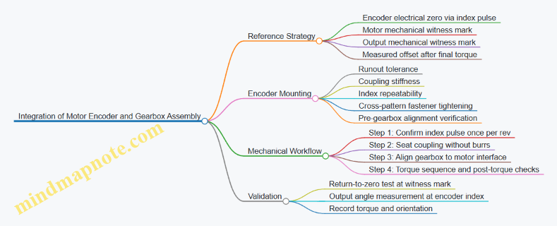
Example Build Notes and Acceptance Checks
Return-to-zero test: rotate to the motor witness mark, then rotate away and return. Acceptance example: encoder angle returns within ±0.05° (adjust to your system resolution). If it fails, address mechanical looseness before touching control software.
Offset repeatability: assemble twice with the same procedure and measure output offset each time. Acceptance example: offsets match within ±0.1° for a compact drone gimbal class build. If offsets vary more, the likely causes are inconsistent seating, bolt torque variation, or misalignment at the motor-gearbox interface.
Engagement feel: rotate the gearbox by hand at low resistance. If the motion feels rough or “notchy,” stop and inspect flexspline seating and wave generator alignment. Roughness changes the effective mapping between motor angle and output angle under load, even if the encoder is perfect.
12.4 Example Build: Test Plan for Torque Ripple and Smoothness
A good test plan separates what you can measure from what you can feel. For torque ripple and smoothness, you want repeatable motion, controlled load, and measurements that can be compared across assemblies.
Test Objectives and What Success Looks Like
Start by defining three measurable outcomes:
- Torque ripple magnitude: the periodic variation in output torque during one gear cycle.
- Smoothness: low-frequency irregularities and discontinuities that show up as spikes in torque, velocity, or position error.
- Repeatability: the same build produces the same signatures when re-tested after disassembly-free handling.
A practical success criterion is not a single number. Use a baseline run from your first “good” assembly, then require later assemblies to stay within a chosen band for ripple amplitude and spike count.
Test Setup and Instrumentation
Use a rigid test bench so the drivetrain is the main source of compliance.
- Drive: motor with the same commutation and current limits used in the real system.
- Load: a controllable brake or friction load to apply a steady resisting torque. Keep it within the actuator’s normal operating range.
- Sensing:
- High-resolution output angle sensor (encoder or resolver) to compute velocity and detect micro-stalls.
- Current sensing on the motor phases to estimate torque, or a torque transducer on the output shaft if available.
- Temperature sensor on the housing or near the bearing seat to correlate drift with thermal effects.
Best practice: log everything with synchronized timestamps. If angle and current are off by even a few milliseconds, ripple phase relationships get messy.
Baseline Conditioning and Repeatability Protocol
Before measuring ripple, condition the mechanism.
- Initial run-in: perform 10–20 cycles of a moderate motion profile under the chosen load.
- Stabilization: wait until temperature change slows, then start the measurement window.
- Repeat runs: run the same profile at least three times without changing alignment or preload.
Example motion profile: a slow constant-velocity sweep over one output revolution, then a return sweep. The return pass helps reveal hysteresis and backlash-related discontinuities.
Measurement Strategy for Torque Ripple
Torque ripple is periodic, so treat it like a signal-processing problem.
- Compute torque from either transducer readings or motor current with a calibrated torque constant and friction compensation.
- Remove the mean torque to focus on the ripple component.
- Use the gear cycle reference: ripple should align with the flexspline engagement pattern and wave generator timing.
Concrete workflow:
- Segment data by output angle bins (for example, 360 bins per output revolution).
- Average torque within each bin across repeated runs.
- Calculate ripple amplitude as the peak-to-peak value of the binned torque curve.
Smoothness Evaluation Beyond Ripple
Smoothness is often where “almost right” assemblies hide.
Measure these indicators:
- Velocity ripple: compute derivative of angle and look for spikes.
- Position error spikes: compare commanded position to measured position after filtering.
- Micro-stall events: detect sudden changes in velocity or torque slope.
A simple rule: if torque ripple looks clean but velocity shows intermittent spikes, the issue is likely friction variation, bearing roughness, or assembly misalignment rather than gear tooth periodicity.
Data Quality Checks
Before trusting results, verify:
- Encoder quantization: ensure resolution is sufficient so velocity spikes are not just digitization.
- Filtering choices: use the same filter settings across runs; document them.
- Load stability: confirm the brake or friction load does not drift during the measurement window.
Mind Map: Test Plan for Torque Ripple and Smoothness
Test Plan Mind Map
Example Test Matrix and Reporting Format
Use a small matrix so you can compare assemblies without drowning in data.
- Load levels: 2 values (light and nominal).
- Motion speeds: 2 values (slow and moderate).
- Direction: forward and reverse.
Report per condition:
- Ripple amplitude (peak-to-peak) with mean and spread across runs.
- Spike count in velocity or position error.
- Temperature at start and end of the measurement window.
Practical Troubleshooting Links Between Symptoms and Causes
- Ripple amplitude high but smoothness metrics clean: tooth engagement geometry or preload distribution.
- Smoothness spikes without strong periodic ripple: bearing surface condition, lubrication inconsistency, or assembly alignment.
- Results drift across runs: thermal effects, load drift, or insufficient run-in.
Keep the test plan consistent. The goal is not to “find the problem” in one run; it’s to make the drivetrain’s behavior comparable, so the next adjustment has a measurable effect.
12.5 Example Build: Troubleshooting Guide for Fit and Control Issues
When a miniaturized harmonic drive and precision servo don’t behave, the failure usually shows up as one of three symptoms: the mechanism feels rough, the controller can’t hold position, or the motion looks fine but the numbers don’t add up. This guide walks from the simplest checks to deeper causes, using a repeatable sequence so you don’t chase ghosts.
Start with Evidence, Not Assumptions
Begin by separating mechanical fit problems from control problems.
- Roughness or binding during slow manual rotation points to tooth engagement, preload seating, bearing alignment, or burrs.
- Good manual feel but poor closed-loop tracking points to sensor scaling, backlash compensation, friction changes, or control loop tuning.
- Tracking degrades as temperature rises points to thermal expansion, lubricant viscosity shift, or fit changes under load.
A practical first step is to run three tests in the same assembly state: (1) manual rotation with power off, (2) motor-driven rotation at low speed with no load, and (3) the same motion under the intended load. Record what changes between tests.
Mechanical Fit Checks That Commonly Cause Trouble
Tooth Engagement and Flexspline Strain
If the flexspline teeth don’t mesh smoothly, you’ll often see inconsistent torque ripple and audible roughness.
- Check for burrs and edge damage on tooth flanks and wave-generator surfaces. Even a tiny burr can create a repeating “catch” once per tooth cycle.
- Verify concentricity and runout of the flexspline and circular spline seats. A small runout can shift engagement depth across rotation.
- Confirm preload seating. If the wave generator or flexspline is not seated squarely, the strain pattern becomes uneven, which increases friction and reduces repeatability.
Example: During a compact gimbal build, tracking error spiked at specific angles. Manual rotation felt smooth, but torque ripple increased at the same angular positions. Inspection found a slight burr on one flexspline tooth edge; removing it reduced both ripple and the control error.
Bearing Seats and Alignment
Misalignment can look like “control trouble” because friction changes with direction.
- Inspect bearing shoulder contact. A gap or high spot can tilt the bearing axis.
- Check shaft straightness and fit. A tight press fit on one side and loose on the other can distort the bearing.
- Look for uneven lubrication film. Dry spots increase stiction, which controllers interpret as disturbance.
Control Issues That Masquerade as Mechanical Problems
Sensor Scaling and Zero References
If the controller thinks the rotor moved when it didn’t, you’ll see steady offsets or oscillation.
- Confirm encoder counts per revolution and gear ratio scaling.
- Re-establish zero after any mechanical disassembly.
- Verify sign conventions for direction and quadrature wiring.
Example: A servo held position but drifted slowly. The mechanism was fine by hand. The root cause was a swapped encoder channel pair, which flipped phase and made the loop fight itself with a small but persistent error.
Backlash and Friction Modeling
Harmonic drives can exhibit direction-dependent friction and small effective backlash.
- Measure backlash experimentally by commanding small reversals and logging the deadband.
- Tune with friction in mind. If the loop is too aggressive, it will “hunt” inside the deadband.
- Use consistent motion direction during calibration so you don’t bake in the wrong baseline.
Systematic Troubleshooting Flow
Use this order so each step reduces the search space.
Mind Map: Fit and Control Troubleshooting
A Concrete Decision Table
If you see X, do Y.
| Observation | Most Likely Cause | First Fix |
|---|---|---|
| Catching at the same angle | Tooth edge burr or engagement mismatch | Deburr and re-inspect tooth edges |
| Direction-dependent stiction | Misalignment or lubrication issue | Re-check bearing seats and lubrication method |
| Steady offset after assembly | Sensor zero or scaling | Recalibrate zero and counts scaling |
| Oscillation near setpoint | Loop too aggressive or backlash deadband | Reduce gains and re-measure deadband |
| Performance worsens with heat | Thermal fit change or viscosity shift | Verify fit clearances and lubrication behavior |
Practical “Do This Next” Checklist
- Clean and inspect tooth edges and wave-generator surfaces for burrs.
- Confirm seating surfaces are free of debris and seated squarely.
- Measure runout and concentricity on the critical interfaces.
- Recalibrate encoder scaling and zero after any mechanical change.
- Measure backlash deadband with small reversals and log it.
- Retune control gains using the same motion profile and direction.
- Repeat the three tests after a short temperature soak to confirm whether the issue is thermal.
Example Resolution Path
A build showed poor repeatability and occasional overshoot. Manual rotation was smooth, but motor-driven motion produced a repeating torque ripple. The team deburred one flexspline tooth edge, re-seated the wave generator, and re-ran the low-speed test. Tracking improved immediately, and the remaining overshoot reduced after re-measuring backlash deadband and lowering the position loop gain slightly. The final confirmation was that performance stayed consistent across the same motion under load, not just in free rotation.