Personal Flight Systems and Jet Suit Engineering Essentials
1. Scope and System Architecture for Wearable Propulsion Platforms
1.1 Defining Personal Flight Systems Requirements and Use Cases
A personal flight system requirement is a statement of what the system must do, under what conditions, and with what measurable success criteria. A use case is the human-centered story that turns those requirements into concrete scenarios, like “hover for 30 seconds while maintaining a stable body attitude.” Together, they prevent the classic mismatch where hardware is built for one interpretation of “stable” and the pilot experiences another.
From Use Cases to Requirements
Start with a small set of operational scenarios that cover the full life of the flight: pre-arm checks, takeoff/hover, maneuvering, landing, and post-flight verification. For each scenario, define:
- Pilot intent: what the pilot tries to achieve (hold position, climb, rotate, translate).
- System outputs: what the system must command (thrust level, attitude targets, actuator commands).
- Constraints: what limits apply (thrust authority, sensor availability, thermal limits, pilot input bandwidth).
- Success criteria: how performance is judged (position error bounds, attitude error bounds, response time, and acceptable oscillation).
A good requirement is testable. If you cannot imagine a ground test or a flight test that would confirm it, it is probably too vague.
Core Use Cases for a Jet Suit
Below is a practical baseline set. Each one should later map to specific control, sensing, safety, and interface requirements.
Pre-Arm and Mode Entry
The pilot powers the system, confirms readiness, and selects an operating mode. The system must verify critical health signals before enabling propulsion.
Example success criteria: propulsion enable is blocked if any required sensor is invalid for more than 200 ms.
Hover Hold
The pilot commands a stable hover while making small corrections. The system must reject disturbances and maintain attitude and position within bounds.
Example success criteria: attitude error stays within ±5° and vertical position error within ±0.5 m for 30 seconds, with no sustained oscillation.
Translation and Maneuvering
The pilot commands forward/backward/side motion and yaw changes. The system must allocate thrust to achieve the commanded motion without exceeding actuator limits.
Example success criteria: commanded yaw rate is tracked within ±10% for a 10-second maneuver, while thrust commands remain within allowable margins.
Transition and Landing
The system handles changes in operating conditions and ensures a controlled descent and shutdown.
Example success criteria: during landing, descent rate follows the commanded profile within ±0.2 m/s and propulsion is reduced to safe levels before final contact.
Post-Flight Data Integrity
The system stores logs needed for review and verifies that critical events are captured.
Example success criteria: every propulsion enable event is logged with timestamps, mode transitions, and fault flags.
Mind Map: Requirements and Use Cases
Turning Scenarios Into Measurable Statements
A useful template is: When a scenario occurs, the system shall achieve a measurable outcome, subject to constraints, while maintaining safety conditions.
Example requirement set for Hover Hold
- When hover hold mode is active and the pilot commands zero translational velocity, the system shall maintain attitude within ±5° and vertical position within ±0.5 m for 30 seconds.
- Subject to thrust authority limits, the system shall avoid sustained oscillations by limiting control output rate changes to a defined maximum.
- While any required sensor is valid, the system shall reject disturbances such that the error does not exceed the bounds even after a step disturbance of defined magnitude.
Practical Use Case Example with Constraints
Consider a “hover hold with small yaw adjustments” scenario. The pilot rotates the suit slowly while expecting the system to keep the body from drifting. That single story forces multiple requirements: yaw tracking must not corrupt position hold, sensor fusion must remain stable during rotation, and the control allocation must respect thrust vector or differential thrust limits.
If you write the use case first, you can then decide what “small yaw adjustments” means in numbers, such as a maximum yaw rate and maximum yaw angle change per second. Those numbers become the basis for controller bandwidth and actuator rate limits.
Requirement Prioritization
Not every requirement has equal weight. Start by prioritizing:
- Safety-critical gating (enable/disable logic, fault handling).
- Stability-critical performance (hover hold error bounds and oscillation limits).
- Command tracking (maneuver response and accuracy).
- Convenience and diagnostics (logging completeness and clear mode feedback).
This ordering keeps early design decisions aligned with what matters most: the system must behave predictably before it behaves impressively.
1.2 Mapping System Boundaries Between Propulsion Power Control and Structure
A jet suit is a chain of responsibilities: propulsion power creates forces, control decides what forces to command, and structure turns those forces into safe motion. Mapping boundaries means drawing a clean line between what the control system promises and what the structure must physically withstand. When that line is fuzzy, you get “works on the bench” designs that fail under real loads, sensor noise, or pilot-induced posture changes.
Foundational Boundary Concepts
Start with three layers that should not be mixed:
- Power and Actuation Layer: fuel flow, electrical power delivery, valves, pumps, motors, and thrust-producing hardware. This layer converts energy into thrust.
- Control and Sensing Layer: sensors, estimation, control laws, mode logic, and command generation. This layer decides thrust setpoints and actuator commands.
- Structural and Mechanical Layer: frame, harness, load paths, mounts, fasteners, and thermal/mechanical interfaces. This layer carries forces and reacts to them.
A boundary is not a physical wall; it is a contract. The contract states what signals cross between layers (commands, feedback, status) and what loads cross between layers (thrust reaction forces, vibration, heat, and mounting stresses).
Define Interfaces as Contracts
For propulsion power control to structure, the most important interface is the force contract: the structure must be designed for the thrust and dynamic loads that the control system can command, including worst-case transients.
To map this, write down three items for each interface:
- Input to the structure: thrust magnitude, thrust direction, thrust ramp rate, and any lateral or torque-producing components.
- Timing and uncertainty: how quickly thrust can change, how much it can overshoot, and what delays exist between command and achieved thrust.
- Output from the structure: measurable effects that the control system can use, such as accelerations, strain-derived proxies, or vibration signatures.
If you cannot measure an output reliably, do not pretend the control system “knows” it. Instead, design the structure to tolerate it and design the control system to avoid commanding beyond safe limits.
Establish Command-to-Load Mapping
Control commands are usually in terms of thrust or attitude targets. Structure cares about forces at mounts and the resulting internal stresses. The mapping step turns “command space” into “load space.”
A practical approach is to define a thrust envelope per operating mode:
- Hover: near-vertical thrust with limited lateral components.
- Transition: changing thrust distribution and ramp rates.
- Cruise or forward motion: sustained thrust with different torque balance.
For each mode, specify:
- Maximum commanded thrust per engine.
- Maximum commanded thrust rate (ramp).
- Maximum allowable thrust asymmetry.
- Maximum expected misalignment between thrust vector and structural axes.
Then translate those into structural load cases: axial loads in harness straps, bending moments at mounts, torsion in frame members, and cyclic fatigue from repeated ramping.
Separate Control Authority from Structural Limits
Control authority is the set of commands the controller can generate. Structural limits are what the structure can safely carry. The boundary is where you enforce the limits.
A clean mapping uses command limiting at the control layer:
- If the controller requests thrust beyond the structural envelope, the command is clipped or reshaped.
- If the controller detects actuator saturation or thrust tracking error, it reduces authority so the structure is not asked to absorb unmodeled transients.
This is not “extra caution”; it is a boundary enforcement mechanism that prevents the control system from accidentally becoming a stress generator.
Mind Map: Boundary Mapping Workflow
Example: Hover-to-Transition Ramp Without Boundary Confusion
Assume the controller uses a thrust command that ramps from 60% to 85% over 0.8 seconds during transition. The structure is designed for a maximum axial load and a maximum bending moment at the engine mounts.
Boundary mapping steps:
- Command envelope: set the maximum ramp rate and maximum overshoot allowed by the actuator model.
- Load translation: compute the worst-case axial and bending loads during the ramp, including the delay between command and achieved thrust.
- Limit enforcement: if tracking error grows (for example, due to valve response lag), the controller reduces the requested thrust rate so the ramp does not exceed the structural load case.
- Feedback reality check: if accelerometer data shows mount vibration spikes, treat that as evidence the structural response is outside the assumed mapping, and adjust the command limits accordingly.
The key is that the controller does not “assume” the structure will magically handle whatever it commands. The structure is designed for the loads the controller is allowed to request, and the controller is constrained to stay inside that envelope.
Example: What Crosses the Boundary and What Does Not
- Crosses boundary: thrust setpoints (control to actuation), actuator status (actuation to control), and measured accelerations (structure to control).
- Does not cross boundary: internal stress states and fatigue life predictions. Those remain structural engineering outputs used to set safe command envelopes, not live control inputs.
When you keep that separation, you get a system that is easier to reason about: control manages behavior within known mechanical capability, and structure provides the physical foundation without pretending to be a sensor.
1.3 Selecting Operating Modes Including Hover Transition and Cruise
Operating modes are not just labels; they define which sensors matter, which control loops run, what limits apply, and what the pilot expects to feel. A jet suit typically needs at least three practical modes: Hover, Transition, and Cruise. Each mode should have explicit entry and exit conditions so the system does not “kindly guess” during the messy middle.
Mode Definitions and Control Responsibilities
Hover mode prioritizes attitude stability and vertical thrust regulation. Lateral motion is allowed but discouraged; the controller should treat sideways drift as a disturbance to be corrected.
Transition mode is the controlled handoff between vertical-dominant control and forward-dominant control. The key challenge is that the same thrust vector changes meaning as airspeed builds and the pilot’s body posture shifts.
Cruise mode emphasizes forward speed regulation and attitude hold with reduced vertical thrust authority. In cruise, the controller can use aerodynamic effects and momentum more effectively, but it must still respect actuator limits and human comfort constraints.
A simple rule helps: the mode determines the control allocation strategy, not just the target commands.
Entry and Exit Conditions That Prevent Mode Thrashing
Mode thrashing happens when the system rapidly switches back and forth due to noisy signals or borderline conditions. Avoid it with hysteresis and a small dwell time.
- Hover to Transition entry: require sustained pilot intent plus a measured condition such as vertical thrust trending downward while forward attitude command increases. Example: the pilot holds a forward input for 0.5 s while vertical thrust demand drops below a threshold.
- Transition to Cruise entry: require airspeed (or a proxy like sustained forward acceleration) above a minimum and attitude error within bounds for a dwell period.
- Cruise to Transition exit: trigger on falling speed below a lower threshold, not the same threshold used to enter.
- Transition to Hover exit: trigger when forward command reduces and vertical thrust demand rises back into the hover authority region.
Use a state machine with explicit guards. The pilot should never need to “fight the mode logic”; the logic should follow the pilot’s intent with predictable constraints.
Mode Logic and What Changes Between Modes
Mind Map: Operating Modes
Mind Map: Operating Modes

Hover Transition: A Practical Blending Strategy
A common mistake is to switch from hover control to cruise control abruptly. Instead, blend the control allocation over a short transition window.
One workable approach is to define a transition blend factor b from 0 to 1:
b = 0: pure hover allocationb = 1: pure cruise allocation
Compute b from measured forward speed proxy and command persistence. Then scale the controller outputs so vertical thrust authority gradually hands off to forward thrust authority.
Example: if the suit has limited thrust margin, the transition controller should cap the rate of change of thrust demand. Otherwise, the system may saturate during the posture change, causing attitude error spikes that the pilot feels as “tugging.”
Cruise: Keeping the Pilot’s Body in the Loop
In cruise, the pilot’s posture changes the effective thrust distribution through harness geometry and body angle. The control system should treat posture-induced effects as measurable disturbances via attitude and rate sensors.
A practical example: if the pilot leans forward, the controller should not immediately chase every small attitude error. Instead, it should maintain a stable attitude envelope while allowing the pilot’s motion to contribute to forward acceleration. That reduces workload and prevents oscillation between pilot correction and controller correction.
Example: A Mode Timeline for One Takeoff and Acceleration
- t = 0 to 2 s: Hover mode. Pilot stabilizes posture; controller holds attitude and regulates vertical thrust.
- t = 2 to 4 s: Transition mode. Forward input persists; blend factor increases; vertical thrust demand decreases smoothly while forward authority increases.
- t = 4 to 8 s: Cruise mode. Speed proxy exceeds minimum; attitude error stays within bounds; controller shifts to forward speed regulation with gentler vertical corrections.
If a sensor fault occurs during transition, the system should drop to a safe mode with conservative authority, because transition is where thrust saturation risk is highest.
Summary of Best Practices for Mode Selection
- Define mode-specific control objectives and allocation strategies.
- Use hysteresis and dwell time to prevent thrashing.
- Blend control authority during hover transition rather than switching abruptly.
- Treat pilot posture effects as disturbances to be managed, not as surprises to be corrected.
- Ensure safety overrides have priority, especially during transition.
1.4 Establishing Engineering Requirements Traceability From Mission Tasks to Tests
Traceability is the habit of answering one question repeatedly: “Which mission need does this requirement prove, and which test will show it?” For personal flight systems, this matters because the same pilot action can stress different subsystems—propulsion, sensing, control, structure, and safety—depending on phase (hover, transition, cruise, landing). A clean traceability chain prevents “requirements that look good” but never get exercised, and it prevents “tests that run” but don’t map to a specific need.
Start with Mission Tasks and Define Observable Outcomes
Mission tasks should be written as actions with measurable outcomes. For example:
- Task: “Maintain hover altitude during a short stop.”
- Observable outcome: altitude error stays within a bound for a specified duration while thrust commands remain within actuator limits.
A practical rule: if an outcome cannot be observed in flight test data (altitude estimate, thrust command, attitude, pilot input), it cannot be a requirement target.
Convert Task Outcomes Into System Requirements
System requirements translate outcomes into constraints on system behavior. Keep them testable by specifying:
- Quantity: what variable (altitude error, attitude rate, thrust margin)
- Bound: allowable range
- Condition: phase, environment, payload state
- Time: duration or settling time
Example requirement:
- “During hover, altitude error shall remain within ±0.5 m for 10 s with pilot input held constant, under nominal battery voltage.”
Then allocate each system requirement to subsystem requirements:
- Sensing requirement: altitude estimate accuracy and latency
- Control requirement: closed-loop stability and disturbance rejection
- Propulsion requirement: thrust tracking error and response time
- Safety requirement: safe thrust reduction on sensor fault
Build Traceability Links Using a Consistent Identifier Scheme
Use stable IDs so links survive edits. A simple pattern works well:
- MT-### for mission tasks
- SR-### for system requirements
- SUB-### for subsystem requirements
- TR-### for test requirements
Example mapping:
- MT-014 “Maintain hover altitude during short stop”
  -> SR-014 “Altitude error within ±0.5 m for 10 s”
  -> SUB-014a “Altitude estimate latency ≤ 50 ms”
  -> SUB-014b “Thrust tracking error ≤ 5% of command”
  -> TR-014 “Hover test with constant input and logged telemetry”
Use a Traceability Matrix to Prove Coverage
A traceability matrix is a table that shows which tests verify which requirements. It should include:
- Requirement ID
- Test ID(s)
- Test phase and setup
- Pass/fail metric
- Evidence location (log set, report section)
Example snippet:
| Requirement ID | Test ID | Metric | Pass/Fail |
|---|---|---|---|
| SR-014 | TR-014 | altitude error over 10 s | max |e_h| ≤ 0.5 m |
| SUB-014a | TR-021 | estimate latency | ≤ 50 ms |
| SUB-014b | TR-030 | thrust tracking RMS | ≤ 5% |
If a requirement has no test, it is not finished. If a test maps to no requirement, it is not finished either.
Mind Map of the Traceability Flow
Mind Map: Mission Tasks to Tests Traceability
Example: From One Mission Task to a Full Verification Set
Consider MT-014 “Maintain hover altitude during a short stop.”
- System requirement SR-014 defines altitude error and duration.
- Sensing subsystem requirement SUB-014a limits estimate latency so the controller reacts before error grows.
- Propulsion subsystem requirement SUB-014b limits thrust tracking error so the controller’s command becomes real thrust.
- Control subsystem requirement SUB-014c limits attitude rate excursions to keep the pilot’s perception consistent and avoid unnecessary structural loads.
- Test requirements include:
- TR-014 hover test for SR-014
- TR-021 latency test for SUB-014a
- TR-030 thrust tracking test for SUB-014b
- TR-040 attitude excursion test for SUB-014c
- TR-050 fault injection test to confirm SR-014 is not blindly “met” during a sensor failure; safety logic must take over.
This is where traceability becomes practical: it prevents a common failure mode where altitude error passes in nominal conditions but the system behaves unpredictably when sensing degrades.
Keep Traceability Alive Through Change Control
Traceability is not a one-time spreadsheet exercise. When any requirement changes, you update the chain and re-check matrix coverage. A lightweight workflow works:
- Change request references the affected requirement IDs
- Impact analysis lists downstream linked IDs
- Verification plan updates test metrics or adds missing tests
A good sign is when a new test proposal can be justified by a specific requirement ID, not by “we should test it because it seems important.”
1.5 Building a Reference Architecture for Jet Suit Subsystems and Interfaces
A reference architecture is a map of how subsystems talk to each other, what they promise, and what they are allowed to do when things go wrong. For a jet suit, the goal is not just neat diagrams; it is predictable behavior across hover, transition, and controlled landing. Start by listing the subsystems you already know you need, then define interfaces that carry the minimum necessary information with clear timing and safety expectations.
Start with Subsystem Boundaries and Responsibilities
Use a “responsibility first” split:
- Pilot Interface: converts human intent into normalized commands.
- Flight Control Computer: estimates state, runs control laws, manages modes.
- Actuation Layer: translates commands into actuator signals and enforces limits.
- Propulsion Powertrain: generates thrust through fuel/power and engine control.
- Sensing and Estimation: provides attitude, rates, altitude, and health signals.
- Safety and Health Monitoring: detects faults and triggers safe responses.
- Data Logging and Telemetry: records events for tuning and post-flight review.
A practical rule: each subsystem should own one kind of decision. For example, the control computer decides “what thrust should be,” while the actuation layer decides “how to realize it within actuator constraints.”
Define Interface Contracts with Timing and Units
Interfaces should be written like contracts, not chat messages. For each interface, specify:
- Signal meaning: physical quantity and sign convention.
- Units and scaling: e.g., thrust in newtons, angles in degrees or radians.
- Update rate: e.g., 200 Hz control commands, 50 Hz health status.
- Latency tolerance: maximum acceptable delay before performance degrades.
- Validity behavior: what happens when data is missing or flagged faulty.
Example: the control computer sends desired thrust per side at 200 Hz. If an actuator feedback signal is invalid, the actuation layer must either hold last safe command or smoothly ramp to a predefined safe thrust, depending on the safety state.
Choose a Data Flow Pattern for Determinism
A clean pattern is sense → estimate → control → allocate → actuate → monitor. Keep the data flow mostly one-directional, with monitoring able to override through explicit safety channels.
- Sense: raw sensor readings with timestamps.
- Estimate: fused state with covariance or confidence flags.
- Control: computes desired forces/torques.
- Allocate: maps desired forces to actuator commands.
- Actuate: drives valves/motors and reports achieved feedback.
- Monitor: checks limits, consistency, and fault conditions.
This structure reduces “mystery coupling,” where a late sensor update changes control behavior without a clear path.
Build the Reference Architecture Mind Map
Jet Suit Reference Architecture Mind Map
Specify Mode-Dependent Interface Behavior
Interfaces must behave differently across modes, but in a controlled way. Define modes such as Ground Standby, Pre-Arm Checks, Hover, Transition, Cruise, and Landing. For each mode, list:
- which sensors are trusted,
- which commands are accepted,
- what limits apply,
- what safety actions are permitted.
Example: in Hover, the controller prioritizes attitude hold and vertical thrust tracking. In Transition, the allocation may reduce authority on one axis to avoid actuator saturation, while safety monitoring becomes stricter about thrust tracking error.
Include a Concrete Interface Example
Consider the interface between Flight Control Computer and Actuation Layer:
- Inputs to Actuation: desired thrust left/right, desired yaw torque, and a mode identifier.
- Actuation outputs: achieved thrust estimate, actuator status, and limit flags.
- Contract: if achieved thrust deviates beyond a threshold for a defined duration, Actuation raises a fault flag to Safety Monitoring.
This keeps the control computer from “fighting” a stuck actuator. The system fails gracefully: control requests stop being blindly executed, and the safety channel can reduce thrust or initiate shutdown.
Validate the Architecture Using Interface Tests
Before any flight-like tuning, test interfaces in isolation:
- Signal sanity: unit checks and sign conventions.
- Timing: verify update rates and timestamp alignment.
- Fault injection: simulate sensor dropout and actuator stiction to confirm the intended fallback behavior.
- Mode transitions: confirm that only the correct commands are accepted in each mode.
A good reference architecture makes these tests obvious. If you cannot write an interface test for a subsystem boundary, the boundary is probably unclear.
Document the Architecture as a Living Artifact
Keep a single source of truth that includes subsystem responsibilities, interface contracts, and mode-dependent behaviors. Version it alongside software and hardware changes so that when a behavior changes, you can trace whether it was a control law update, an interface contract change, or a safety policy adjustment.
Mind maps help you see the whole system; interface contracts help you build it without surprises. Together, they turn “it works on the bench” into “it behaves predictably when reality gets messy.”
2. Human Factors Foundations for Wearable Flight Control
2.1 Human Sensory Limits for Motion Perception and Feedback Interpretation
Designing a jet suit control interface means respecting what the pilot’s body can reliably sense. The control system can be mathematically correct and still feel wrong if the pilot cannot interpret motion, timing, or force cues. This section translates human sensory limits into practical design constraints for wearable propulsion.
Core Perception Channels and What They Can Trust
Humans combine multiple signals: vision for orientation and motion, vestibular organs for acceleration and rotation, proprioception for body position and effort, and touch for contact forces. Each channel has limits in bandwidth, latency, and ambiguity.
Vision is strong for relative motion and stable reference frames, but it struggles when the scene lacks cues or when motion is fast enough that the pilot’s eye tracking can’t keep up. Vestibular sensing is good at detecting angular motion and certain acceleration patterns, but it can be confused by sustained acceleration and by mismatches between expected and actual motion. Proprioception is excellent for detecting effort and joint loading, yet it is slower for estimating absolute body pose when the suit changes load paths.
A useful rule: treat vision as the “high-level truth source” when cues exist, and treat vestibular and proprioceptive signals as “fast but sometimes biased” sources. Your feedback design should not require the pilot to solve a puzzle under stress.
Latency and Timing: The Hidden Enemy
Perception is not instantaneous. Even when sensors and control loops are fast, the pilot’s interpretation lags. If feedback arrives late relative to the pilot’s input, the pilot compensates in the wrong direction. If feedback arrives too early or too strongly, the pilot may over-correct.
Practical implication: align feedback timing with the pilot’s action timing. For example, if the pilot commands a pitch change by shifting posture, the suit should produce a corresponding attitude response quickly enough that the pilot’s vestibular system can associate the motion with the command. Otherwise, the pilot experiences “I moved, but the suit didn’t,” which leads to corrective oscillation.
Motion Perception Thresholds and Ambiguity
Small changes can be below detection thresholds, especially when multiple cues compete. For instance, a slight thrust change may be sensed as effort through the harness, but the resulting body acceleration might be too small to be clearly felt by the vestibular system. Conversely, a strong acceleration might be felt, but the pilot may not distinguish whether it came from thrust, posture, or external disturbance.
This is why feedback should be redundant but not conflicting. If the suit increases thrust, the pilot should receive consistent cues: attitude change (visual), acceleration cue (vestibular), and load cue (haptic/tactile). If only one channel changes, the pilot may interpret the event incorrectly.
Feedback Interpretation: Mapping Sensation to Meaning
The pilot’s brain interprets feedback through learned associations. If the mapping between command and sensation changes across operating modes, the pilot must relearn it mid-flight. That’s a great way to turn “control” into “guessing.”
A stable mapping example: when the pilot increases forward intent, the suit should consistently produce forward pitch-up or forward acceleration depending on the chosen control mode. If sometimes it changes attitude and other times it changes only thrust, the pilot’s internal model breaks.
Harness and Contact Forces as a Communication Channel
Touch and pressure cues can be powerful because they are continuous and local. But they depend on fit and load path. A harness that shifts during motion changes the pressure distribution, so the same thrust command produces different sensations.
Design constraint: keep contact mechanics consistent. For example, if the suit uses a strap tension cue to indicate thrust level, ensure that strap tension changes monotonically with thrust and that the harness does not “re-seat” during normal maneuvers. Otherwise, the pilot learns the wrong relationship.
Mind Map: Sensory Limits and Feedback Design Targets
Example: Hover Transition Without Cue Confusion
Imagine a pilot shifting posture to initiate a hover-to-forward transition. If the suit first changes thrust but delays the resulting pitch response, the pilot feels increased harness load but does not sense the expected attitude change. The pilot then adds more input, causing a larger thrust change, and the suit finally pitches—now the pilot is “late” and over-corrects.
A better approach is to coordinate cues: start the attitude response promptly while thrust ramps smoothly. The pilot should feel a consistent sequence: command → early attitude cue → increasing load cue. This reduces the need for the pilot to infer what the suit is doing.
Example: Mode Switching with Meaning Preservation
Suppose the suit has an assisted recovery mode that changes control authority. If the pilot’s same posture input suddenly produces a different direction of motion, the pilot’s internal model fails. Even if the recovery mode is safer, it can still be destabilizing.
To preserve meaning, keep the mapping from pilot intent to the primary motion axis consistent across modes. The recovery mode can change gains or limits, but the directionality of response should remain predictable. The pilot should recognize the “shape” of the response even when the “strength” changes.
Practical Checklist for Designers
- Identify which channel carries the primary cue for each control variable (attitude, acceleration, thrust state).
- Ensure feedback timing supports cue association with the pilot’s input.
- Keep command-to-sensation mapping consistent across modes.
- Make harness contact cues monotonic and fit-stable.
- Avoid relying on a single sensory channel when cues can be ambiguous.
When these constraints are met, the pilot’s perception becomes a reliable part of the control loop rather than a source of uncertainty. The suit then behaves like a tool the pilot can learn quickly, not a system the pilot must constantly interpret.
2.2 Pilot Workload Management Using Interface Design and Control Allocation
Pilot workload management is about keeping the pilot’s attention where it matters: monitoring key states, making intentional commands, and recovering from mistakes without fighting the interface. In a jet suit, the interface and control allocation are tightly coupled because the pilot’s inputs directly shape thrust distribution, attitude response, and system mode transitions.
Foundational Principles for Workload Control
Start with a simple workload model: workload rises when the pilot must (1) interpret ambiguous feedback, (2) plan multi-step actions, (3) correct overshoot caused by poor control authority mapping, or (4) handle unexpected mode behavior. Interface design reduces interpretation and planning effort; control allocation reduces correction effort.
A practical rule is to separate “what the pilot intends” from “what the system does.” The pilot intends a goal (hold altitude, rotate left, slow down). The system executes via allocation (how much thrust each actuator gets) and stabilization (how the body stays within limits). When those layers are blurred, the pilot ends up doing extra work to compensate.
Interface Design That Reduces Interpretation Effort
Use feedback that matches how people naturally check status. For example, altitude and vertical thrust should be communicated in a way that supports quick comparisons: “current vs target,” not just raw numbers. If the suit has a target-hold mode, show the target reference clearly and keep the pilot’s attention on deviations.
Control mapping should also be consistent across modes. If the same input produces different effects in different modes, the pilot must re-learn the mapping under stress. A concrete example: if a trigger increases thrust in hover but increases forward acceleration in cruise, the interface should either (a) keep the trigger’s meaning consistent (e.g., always “increase commanded vertical thrust component”) or (b) make the mode change visually and audibly obvious before the mapping changes.
Finally, reduce the need for mental filtering. If sensor data is noisy, don’t force the pilot to average it mentally. Apply smoothing and present stable indicators, while still showing meaningful changes quickly enough for control.
Control Allocation That Reduces Correction Effort
Control allocation decides how commanded forces and moments become actuator commands. Workload drops when the allocation behaves predictably near limits. Two common workload spikes are saturation and coupling surprises.
Saturation example: Suppose the pilot commands a rapid pitch-up while the suit is already near thrust limits. If allocation simply clips actuator commands, the pilot sees “input in, attitude not responding,” which triggers repeated corrections. A better approach is to communicate the effective authority through the feel of the control response: reduce commanded response rate smoothly and bias the system toward maintaining stability rather than chasing the impossible.
Coupling example: If yaw commands unintentionally create roll, the pilot must counter-roll, increasing workload. Allocation can minimize coupling by solving for actuator commands that achieve the requested moment with constraints that limit unwanted axes. Even if perfect decoupling is impossible, the system should keep coupling small and consistent so the pilot can learn a stable compensation pattern.
Mode Transitions That Prevent Surprise Work
Mode transitions are where pilots often lose time. The interface should make transitions legible and the control laws should avoid discontinuities.
A concrete hover-to-cruise example: when the pilot releases a hover hold and requests forward motion, the system should ramp the thrust distribution and attitude targets over a short, deterministic window. During that window, the pilot should still be able to make small corrections without fighting a sudden change in control authority.
Similarly, assisted recovery modes should be designed so the pilot doesn’t have to “undo” the system. If recovery engages, the pilot’s inputs should either (1) be interpreted as “continue the recovery” or (2) be temporarily limited to safe adjustments, with clear feedback indicating which interpretation is active.
Practical Allocation Strategies for Workload
Use a layered approach: an inner stabilization loop that handles fast dynamics, and an outer loop that tracks pilot goals. Workload improves when the outer loop is forgiving and the inner loop is strict.
Example allocation policy:
- Convert pilot intent into desired body rates or attitude angles.
- Compute required moments.
- Allocate moments to actuators with constraints that prioritize stability and limit abrupt actuator changes.
- If constraints bind, prioritize maintaining safe attitude and vertical thrust, then reduce the requested moment magnitude smoothly.
This policy prevents the pilot from repeatedly “pushing harder” to overcome saturation.
Pilot Workload Management Mind Map
Mind Map: Workload Management Through Interface and Allocation
Worked Example: Keeping Workload Low During a Turn
Assume the pilot requests a left turn while maintaining altitude. The interface converts the pilot’s yaw intent into a desired yaw moment and a small coordinated roll moment to keep the turn efficient. Control allocation then distributes thrust changes to achieve the yaw moment while constraining roll coupling and limiting actuator rate changes.
If the suit approaches thrust limits, the allocation reduces the achievable yaw moment smoothly and maintains altitude first. The pilot experiences a turn that may be less aggressive than requested, but it remains stable and consistent, so the pilot doesn’t need repeated corrective inputs to “force” the response.
The result is a workload profile dominated by monitoring and intentional small corrections, not by fighting the interface or compensating for unpredictable coupling.
2.3 Ergonomics of Harness Fit Load Paths and Posture Stability
A jet suit’s harness is not just “straps that hold things.” It is the interface that turns pilot intent and propulsion forces into predictable motion. Good ergonomics starts with fit, then follows the load paths those forces take through the body, and ends with posture stability that keeps control inputs consistent.
Foundational Fit Principles for Consistent Control
Begin with repeatable placement. If the harness shifts a few centimeters between flights, sensor-to-body alignment changes, and the same control input can produce a different feel. Fit should be adjustable in at least three directions: vertical position (so the suit sits consistently), circumferential tension (so it doesn’t loosen with movement), and fore-aft alignment (so the thrust reaction doesn’t “walk” the harness).
A practical check is the “two-minute settle.” After tightening, stand in a neutral stance, then perform slow knee bends and gentle torso rotations. If the harness migrates or wrinkles concentrate at one spot, you have a fit problem that will become a control problem.
Load Path Mapping from Thrust to Body
Load paths describe where forces travel: from propulsion thrust into the frame, from the frame into the harness, and from the harness into the body. The goal is to distribute loads across strong body regions and avoid concentrating them on soft tissue.
Use a simple load-path worksheet:
- Primary reaction direction: where thrust pushes the suit (often backward and upward relative to the pilot).
- Primary support regions: areas that can carry tension/compression (typically shoulders, upper torso, and hip/waist structures).
- Constraint points: where the harness prevents unwanted motion (for example, preventing the frame from rotating relative to the torso).
- Failure points: where discomfort or slippage begins (common culprits: collarbone edges, lower back hotspots, and strap edges).
A good harness makes the body feel “held” rather than “pinched.” If the pilot reports a sharp point of pressure, that usually means the load path is too narrow.
Posture Stability Through Constraint and Freedom
Posture stability is about controlling degrees of freedom. The harness should allow motion that supports natural stance while constraining motion that destabilizes control.
A useful way to think about it is to separate:
- Allowed motion: small torso adjustments that help the pilot balance.
- Constrained motion: large translations or rotations that change the pilot’s reference posture.
For example, if the harness allows the frame to rotate forward under thrust, the pilot will compensate by leaning back, which increases muscle effort and changes how inputs map to motion. Instead, design strap geometry and attachment stiffness so the frame’s rotation is resisted by upper torso support and hip anchoring.
Mind Map: Harness Fit Load Paths and Posture Stability
Example: Diagnosing a “Leaning to Fly” Problem
A pilot reports that hovering feels fine at first, then they start leaning backward to keep altitude. The harness feels tight at the shoulders but oddly loose at the hips.
A systematic diagnosis:
- Check migration: after a few minutes, does the harness ride up? If yes, the upper support is doing too much.
- Inspect load distribution: shoulder pressure suggests the load path is concentrated at the top rather than shared with the hip/waist.
- Evaluate rotational constraint: if the frame rotates forward under thrust, backward leaning becomes a compensatory control strategy.
- Adjust fit and geometry: increase hip anchoring tension and ensure strap routing resists forward rotation without creating collarbone edge pressure.
The fix is not “make it tighter everywhere.” It is to reroute the load path so the body experiences broad support and the frame’s motion relative to the torso is limited.
Example: Preventing Strap Edge Hotspots
During ground tests, a pilot notices a narrow hot line where a strap edge contacts the torso. Even if the pilot can tolerate it, the hotspot can change posture over time.
A practical remedy:
- Increase contact area at the strap edge using a wider interface pad or smoother strap geometry.
- Reposition the strap so it sits on a load-bearing region rather than near a bony prominence.
- Verify that tightening does not pull the strap across the skin during torso motion; if it does, the harness needs a different routing angle or a secondary stabilizing strap.
When comfort improves, posture stability usually improves too, because the pilot stops making subtle adjustments to avoid pressure.
Practical Fit Verification Checklist
Before any flight session, verify:
- The harness sits at the same vertical level each time.
- No single point carries disproportionate pressure.
- The harness does not migrate during slow bends and rotations.
- The pilot can maintain neutral stance without compensatory leaning.
- Hip support shares load with upper torso support.
Ergonomics is successful when the pilot’s body feels like a stable reference frame, not a moving platform. That stability is what makes control inputs predictable and repeatable.
2.4 Training and Procedure Design for Safe Operation and Recovery Actions
Safe operation training for a jet suit is less about memorizing steps and more about building reliable behavior under stress. Procedures should therefore be written to match how people actually notice problems, decide what to do, and act with limited attention.
Foundations of Procedure Design
Start with a simple chain: stimulus → recognition → decision → action → verification. Training should rehearse each link, because failures often happen at the recognition stage (wrong interpretation) or the verification stage (no confirmation that the action worked).
Use phase-based procedures aligned to how the system behaves: pre-activation checks, takeoff/hover, maneuvering, landing, and post-flight. Each phase gets a short “what to watch” list and a “what to do if it happens” list. For example, during takeoff you emphasize thrust response and attitude stability; during landing you emphasize descent control and safe shutdown timing.
Write procedures with clear triggers. A trigger is a condition that can be observed without guesswork, such as “uncommanded roll increasing for more than two seconds” or “loss of expected thrust response after pilot command.” Avoid vague triggers like “feels wrong.”
Finally, include verification steps that are measurable. “Confirm stability” becomes “confirm attitude error is decreasing and thrust command is within expected range.” This reduces the chance of repeated actions that make the situation worse.
Training Structure That Builds Automaticity
Train in layers: first with the suit powered down (dry runs), then with limited actuation (ground tether or restricted thrust), then with full operation under controlled boundaries.
- Dry Run Training: Practice the procedure flow using a checklist and verbal callouts. Example: the trainee runs the recovery sequence while the instructor simulates sensor faults by announcing “rate sensor dropout” at specific times.
- Ground Restricted Training: Practice the same flow with the system active but constrained. Example: limit maximum thrust so the trainee can focus on recognition and correct decision timing.
- Scenario Training: Use repeatable scenarios that map to specific triggers. Example: “hover oscillation begins after a sudden input” tests whether the trainee reduces command aggressiveness and switches to the correct assist mode.
Keep sessions short and consistent. If a trainee must read the checklist every time, the procedure is not yet a behavior. The goal is that the trainee can start the right recovery action within a few seconds of trigger recognition.
Recovery Actions as a Decision Tree
Recovery actions should be designed as a decision tree rather than a single script. Different faults call for different priorities: stabilize first, then reduce energy, then shut down if needed.
A good recovery tree separates control authority problems from sensor/estimation problems and from power/actuation problems.
Mind Map: Safe Operation and Recovery Procedure Flow
Concrete Example Scenarios
Example 1: Hover Oscillation After Aggressive Input
- Trigger: attitude error oscillation grows while pilot input rate remains high.
- Decision: stabilize first by reducing input rate and centering commands.
- Action: engage the appropriate hold/assist mode if available.
- Verification: confirm oscillation amplitude decreases and thrust command returns to a stable band.
Example 2: Loss of Expected Thrust Response
- Trigger: commanded thrust change does not produce the expected acceleration/attitude response within a defined time window.
- Decision: treat as actuator or power delivery issue.
- Action: reduce commanded thrust, transition to a controlled descent, and prepare for shutdown if stability cannot be restored.
- Verification: confirm descent rate and attitude remain within safe limits before continuing.
Example 3: Sensor Dropout During Maneuvering
- Trigger: estimator confidence drops or a specific sensor health flag indicates dropout.
- Decision: switch to a safe mode designed for degraded sensing.
- Action: reduce maneuver complexity, return toward a stable hover/landing posture.
- Verification: confirm mode/state change and that control outputs remain within limits.
Debrief and Procedure Improvement Loop
After each drill, review only what matters: the trigger the trainee used, the decision they made, and the verification they performed. If the trainee acted correctly but verified incorrectly, the procedure needs clearer measurable checks. If the trainee verified correctly but chose the wrong branch, the trigger definitions need tightening. This keeps training grounded in observable behavior rather than “good effort.”
2.5 Human Error Modes and Mitigation Through Control System Design
Human error in personal flight systems is rarely a single “mistake.” It is usually a chain: perception slips, interpretation lags, action is delayed or misapplied, and the control system either amplifies the chain or breaks it. This section maps common error modes to specific control-system mitigations, using examples that fit wearable propulsion constraints.
Error Modes That Show Up in Real Operations
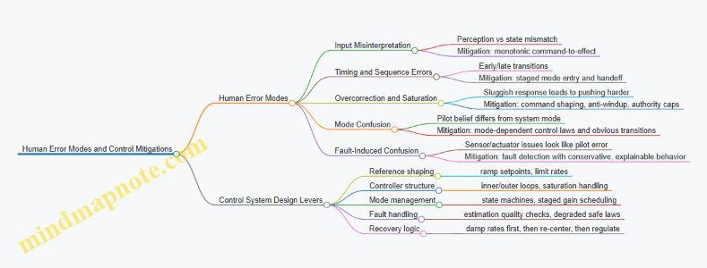
Mode 1: Input Misinterpretation
Pilots may read a cue incorrectly—altitude feels “about right,” but the system is actually descending. In a jet suit, the body’s posture and the pilot’s vestibular sense can disagree with the vehicle state.
Mode 2: Timing and Sequence Errors
A common pattern is acting too early or too late during transitions, such as attempting a thrust increase before the hover controller has stabilized.
Mode 3: Overcorrection and Control Saturation
When response feels sluggish, pilots push harder. If the controller saturates, the pilot’s additional input no longer produces proportional effect, which increases oscillation risk.
Mode 4: Mode Confusion
Wearable systems often have distinct behaviors: hover hold, assisted recovery, manual attitude control. If the pilot believes they are in one mode while the system is in another, the control law may fight the pilot.
Mode 5: Fault-Induced Confusion
A sensor dropout or actuator lag can look like “pilot error” because the aircraft doesn’t respond as expected.
Control System Mitigations That Reduce Error Impact
Mitigation 1: Make the System “Hard to Misread” Control design can reduce ambiguity by shaping response so that the pilot’s expected action produces a consistent outcome. For example, in hover hold, command-to-effect should be monotonic: increasing the thrust request should not initially cause a descent.
Example: If the pilot presses a trigger to request more lift, the controller ramps thrust setpoint with a short, predictable slope and limits the rate of change. Even if the pilot’s perception is off by a few inches, the system behavior stays interpretable.
Mitigation 2: Use Mode-Dependent Control Laws With Clear Transitions
Mode confusion is best handled by designing transitions that are physically obvious. A hover-to-cruise switch should include a controlled handoff: the controller gradually shifts authority from vertical stabilization to forward acceleration tracking.
Example: When entering hover hold, the controller first estimates attitude and vertical velocity, then gradually tightens gains. The pilot feels a “settling” phase rather than an abrupt change.
Mitigation 3: Add Rate and Authority Limits That Prevent Overcorrection
Saturation is where pilot intent stops matching system output. The controller should manage saturation proactively using command shaping and anti-windup strategies.
Example: If the pilot commands a large pitch-up, the controller caps the commanded angular acceleration and uses an anti-windup mechanism so integral terms do not accumulate during saturation. The result is less rebound when the pilot eases off.
Mitigation 4: Detect and Contain Faults So They Don’t Masquerade as Pilot Error
Fault detection should trigger behavior that is safe and also explainable through system response. For instance, sensor dropout should not silently switch to a degraded controller that behaves unpredictably.
Example: If inertial estimation quality drops, the system can reduce thrust authority and switch to a conservative stabilization mode that prioritizes maintaining attitude and limiting vertical speed. The pilot experiences a clear “slower, steadier” response rather than a confusing mismatch.
Mitigation 5: Build Recovery Behaviors That Are Triggerable Without Perfect Timing
Humans are not good at precise timing under stress. Recovery logic should tolerate delayed or imperfect inputs.
Example: If the pilot releases controls or presses a recovery gesture, the controller enters a hold-and-stabilize sequence that first damps angular rates, then re-centers attitude, then resumes vertical regulation. The pilot doesn’t need to know the exact state; the system does the first steps.
Mind Map: Error Modes and Control Design Responses
Practical Example Walkthrough: From Error to Safe Containment
Consider a pilot initiating hover hold while the system is still settling from a prior maneuver. Without safeguards, the pilot’s first thrust inputs can excite vertical oscillations. With the mitigations above, the controller stages mode entry: it estimates vertical velocity, ramps thrust authority gradually, and limits vertical speed. If the pilot overcorrects, saturation limits prevent integral buildup, so the system returns to the target without a large rebound. If a sensor quality check fails during the transition, the controller switches to a conservative stabilization law that prioritizes attitude and limits vertical motion, reducing the chance that the pilot keeps “chasing” a nonresponsive system.
The key idea is simple: control design should assume imperfect human inputs and imperfect timing, then shape system behavior so that errors become smaller, slower, and easier to recover from.
3. Propulsion Hardware Fundamentals for Jet Suit Engineering
3.1 Thrust Generation Principles and Nozzle Selection Considerations
Thrust is the reaction force produced when a propulsion system accelerates a working fluid. In a jet suit context, the “working fluid” is typically air, and the propulsion system adds energy so the air exits at higher velocity than it enters. The core idea is simple: if you can move mass faster, you get a push backward. The engineering challenge is making that push controllable, efficient, and safe while fitting inside a wearable package.
Thrust Fundamentals from Momentum to Usable Force
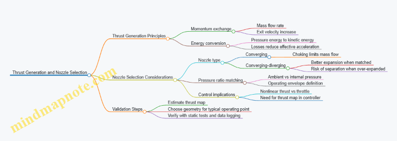
Start with the momentum view: thrust equals the rate of change of momentum of the fluid. Practically, you can think of thrust as depending on two levers: how much air you move (mass flow rate) and how much you increase its exit speed. A useful mental model is that doubling mass flow can roughly double thrust if exit velocity rise stays similar.
Next, connect thrust to nozzle behavior. A nozzle converts pressure energy into kinetic energy. If the nozzle is matched to the operating pressure conditions, it accelerates the flow effectively. If it is mismatched, some energy remains as pressure rather than velocity, and thrust drops.
A third lever is losses. Even if the nozzle geometry looks right, friction in the duct, mixing losses, and heat transfer can reduce the effective energy available for acceleration. That’s why nozzle selection is never just “pick the smallest exit.” It’s about matching the nozzle to the expected pressure ratio and flow regime.
Nozzle Types and What They Trade
Nozzles are usually categorized by how they handle pressure differences between the inside and the outside environment.
- Converging nozzles accelerate flow when the pressure ratio is high enough, but they can become limited by choking. Once choked, further increases in upstream pressure don’t increase mass flow much, which can cap thrust.
- Converging-diverging nozzles can expand the flow more efficiently when the pressure ratio supports it. They can produce higher thrust at certain conditions, but they are more sensitive to operating point and can suffer from flow separation if the expansion is excessive.
- Fixed vs. variable geometry: fixed nozzles are simpler and lighter, but they must be sized so the suit’s typical operating points land in a favorable region. Variable nozzles add complexity and actuation loads, so they are usually reserved for systems that truly need wide operating coverage.
Matching Nozzle to Operating Pressure Ratio
Nozzle performance depends on the pressure ratio between the nozzle inlet (or combustor/duct stagnation pressure) and the ambient pressure. In a wearable system, ambient pressure changes with altitude and local conditions, and internal pressure changes with throttle and control mode.
A practical selection workflow is to define a thrust map target: for each expected operating condition, estimate the required thrust and allowable efficiency loss. Then choose nozzle geometry that yields good expansion for the majority of the operating envelope. If your control system frequently runs near a single thrust level, a fixed nozzle can be optimized around that point.
Choking and Why It Matters for Control
Choking occurs when the flow reaches sonic conditions at the throat, limiting further mass flow increases. For control, choking is both helpful and tricky. Helpful because it can make thrust less sensitive to small upstream pressure changes. Tricky because it can create a nonlinearity: beyond a certain throttle command, thrust may not increase proportionally.
That nonlinearity must be reflected in the control allocation and thrust command mapping. Otherwise, the pilot interface can feel “mushy” or inconsistent: the same input produces different thrust increments depending on whether the nozzle is choked.
Mind Map: Thrust Generation and Nozzle Selection
Example: Choosing Between Converging and Converging-Diverging
Assume a suit operates most of the time in a narrow thrust band for hover and low-speed maneuvering. If the internal stagnation pressure relative to ambient stays high enough to choke a converging nozzle, thrust will be capped and throttle-to-thrust gain will flatten. In that case, a converging-diverging nozzle may provide better thrust responsiveness by allowing additional expansion when the pressure ratio supports it.
However, if the suit frequently transitions through conditions where the pressure ratio drops, a converging-diverging nozzle can move away from its best expansion point. The result can be reduced efficiency and potentially unstable flow behavior. The selection decision becomes: optimize for the dominant operating region, then ensure the controller handles the remaining regions with a calibrated thrust map.
Example: Using a Simple Thrust Map for Control Consistency
Suppose you measure static thrust at several throttle settings and record the corresponding nozzle operating state (for instance, whether the throat is choked). You then fit a piecewise relationship: one slope for the choked region and another for the unchoked region. In operation, the controller uses the current estimated internal pressure to select the correct segment. The pilot experiences smoother thrust increments because the mapping respects the nozzle physics rather than pretending the system is linear.
In short, thrust generation is momentum plus energy conversion, and nozzle selection is the art of matching pressure-driven acceleration to a changing operating environment—then teaching the control system the same physics so the pilot gets predictable response.
3.2 Fuel and Power Delivery Components Including Valves Regulators and Lines
Fuel and power delivery is where “it should work” meets “it actually works while strapped to a human.” This section treats the delivery chain as a set of functions: store energy, condition it, meter it, distribute it, and keep it safe when something goes wrong. The goal is predictable thrust response with minimal surprises in pressure, flow, temperature, and electrical behavior.
Functional Breakdown from Tank to Thrust
Start with the simplest mental model: the propulsion unit needs a controlled energy input. For fuel systems, that means stable pressure and correct flow to injectors or burners. For electrical systems, it means stable voltage/current to motors, pumps, controllers, and ignition subsystems.
A practical way to design is to define these interfaces:
- Energy source interface: battery pack terminals or fuel tank outlet.
- Conditioning interface: regulator output (electrical) or pressure control output (fuel).
- Metering interface: valve or pump control element that sets flow.
- Distribution interface: lines and manifolds that deliver to the propulsion unit.
- Feedback interface: sensors that confirm pressure/flow/voltage/current.
If you can name these interfaces, you can test them independently.
Valves as Flow Governors
Valves are not just on/off switches. In wearable propulsion, they often act as rate limiters and response shapers.
Key valve roles:
- Shutoff: isolates the system during faults or pre-arm.
- Regulation: maintains target flow or pressure by modulating opening.
- Dosing: provides repeatable metering during specific phases like spool-up.
Example: Suppose the controller commands a thrust step. If the fuel valve opening is too aggressive, pressure overshoots, then undershoots as the system hunts. A better approach is to pair valve dynamics with a pressure regulator and tune the control loop so the commanded thrust maps to a controlled pressure trajectory rather than a raw valve position.
Valve selection considerations:
- Response time: affects control stability.
- Leakage: matters for safety and for preventing unintended ignition or drag.
- Cv or flow coefficient: determines how much pressure drop you need for a given flow.
- Materials compatibility: fuel chemistry and temperature exposure.
Regulators as Pressure and Voltage Stabilizers
Regulators convert a variable input into a controlled output. In fuel systems, regulators manage pressure against changing demand. In power systems, regulators manage voltage/current against battery sag and load transients.
Fuel pressure regulation typically uses one of these patterns:
- Pressure regulator with feedback: maintains setpoint using a control element.
- Pump plus relief: pump sets flow, relief maintains pressure ceiling.
Example: During hover, demand is steady. During transition, demand changes quickly. A regulator that is stable under steady load might still oscillate under fast demand changes. The fix is to ensure the regulator’s control bandwidth and the downstream line volume do not create a resonance with the valve and controller.
Electrical regulation considerations:
- Current limiting to protect power electronics.
- Transient response to prevent controller resets.
- Ripple and noise management so sensor readings remain trustworthy.
Lines as the Hidden Spring and Damping
Lines are often treated as plumbing, but they behave like dynamic elements. A line has volume (compressibility), friction (damping), and sometimes compliance (expansion). Those properties shape pressure and flow response.
Design steps that prevent surprises:
- Estimate line volume between regulator and propulsion unit.
- Estimate pressure drop at expected flow rates.
- Check thermal expansion and routing constraints.
- Plan for air or vapor management if applicable.
Example: If a line is long and compliant, a valve step can create a delayed pressure rise at the injector. The controller sees pressure late, so it overcorrects. Shortening the effective run, adding a local manifold volume strategy, or adjusting control loop timing can restore predictable response.
Routing best practices:
- Avoid sharp bends that increase friction and trap bubbles.
- Secure lines to prevent rubbing and fatigue.
- Keep hot and cold sections separated to reduce thermal gradients.
Safety Interlocks in the Delivery Chain
Safety is easiest when it is layered. A typical layered approach:
- Primary shutoff valve that closes on fault.
- Pressure relief path that prevents overpressure.
- Electrical protection such as fusing and current limiting.
- Sensing and plausibility checks so the controller can detect stuck valves, sensor dropout, or abnormal pressure.
Example: If a pressure sensor reads “normal” but the valve is commanded closed, the system should flag inconsistency. That check prevents the controller from trusting a single measurement while ignoring the commanded state.
Mind Map: Fuel and Power Delivery Components
Integrated Example Workflow for Component Selection
- Define the required thrust response profile and translate it into demand: target fuel flow/pressure or electrical current/voltage.
- Choose a valve strategy that can produce the needed response time without excessive overshoot.
- Select a regulator that remains stable with the expected line volume and valve dynamics.
- Size lines for acceptable pressure drop and manageable dynamic delay.
- Add sensors so the controller can confirm the delivery chain is behaving as commanded.
- Implement safety interlocks that isolate energy and prevent overpressure or electrical overload.
This workflow keeps the system testable: you can validate valve behavior first, then regulator response, then line dynamics, and finally closed-loop thrust tracking.
3.3 Intake Exhaust Routing and Heat Management for Wearable Packaging
Wearable propulsion packaging has two routing jobs that fight each other: moving air and moving heat. Intake and exhaust paths must support stable engine operation while keeping skin temperatures, electronics temperatures, and structural temperatures within limits. The trick is to treat routing as a system, not a set of tubes.
Intake and Exhaust Routing Foundations
Start with the airflow requirements of the propulsion unit. Intake routing should deliver air with minimal pressure loss and minimal temperature rise. Exhaust routing should remove hot gases without creating backpressure that forces the propulsion unit to work harder. In practice, “minimal” means you design for straight-ish paths, smooth transitions, and controlled bends.
A useful mental model is to separate routing into three layers:
- Gas path: where air and exhaust actually flow.
- Thermal path: where heat travels by convection, conduction, and radiation.
- Mechanical path: where vibration and loads travel through mounts and flexible sections.
If you only optimize the gas path, you may accidentally route heat into the harness. If you only optimize thermal isolation, you may increase pressure losses and reduce thrust. Good routing balances both.
Designing the Intake Path
Intake air should be protected from recirculation. Recirculation happens when exhaust plumes wrap around and re-enter the intake, raising intake temperature and reducing performance. To prevent this, keep intake openings away from exhaust discharge zones and avoid routing that creates “short-circuit” flow.
Pressure loss is the next constraint. Every bend, contraction, and rough surface adds loss. An easy example: if you replace a 90-degree elbow with a larger-radius bend, you often reduce loss enough to improve stability at low throttle. The same principle applies to flexible hoses: long, tightly curved sections tend to increase losses and can trap condensation.
Thermal considerations for intake are usually secondary to pressure loss, but not negligible. If intake tubing runs near hot exhaust, it will absorb heat and raise intake temperature. Even a modest temperature rise can reduce density and change control behavior. Route intake away from exhaust, or use a thermal barrier where separation is impossible.
Designing the Exhaust Path
Exhaust routing must handle high temperatures and flow pulsations. Backpressure is the enemy of consistent thrust. To reduce backpressure, keep exhaust paths short, avoid sharp restrictions, and ensure the discharge has a clear outlet.
A practical example: if you route exhaust through a narrow channel to “hide” it, you may create a restriction that increases backpressure. The propulsion unit compensates by changing operating conditions, which can increase heat generation further. The result is a loop: restriction raises heat, heat raises losses, and the system gets harder to control.
Exhaust also needs vibration-aware mounting. Hot gas lines expand, and vibration can fatigue mounts. Use compliant sections where appropriate, but constrain them so they do not rub on harness material. A simple check is to simulate or measure relative motion under expected vibration and confirm there is no contact under worst-case engine torque.
Heat Management Through Routing and Separation
Heat management is not only about insulation; it’s about where heat goes. Use routing to create separation distances between hot exhaust components and skin-facing or electronics-facing areas.
A systematic approach:
- Source: identify the hottest surfaces and their temperature range during steady operation.
- Conduction routes: find structural members that connect hot and cool regions.
- Convection routes: identify airflow patterns around the suit that can carry heat away.
- Radiation routes: account for line-of-sight between hot surfaces and nearby components.
Then apply targeted measures:
- Thermal barriers between exhaust and harness zones.
- Heat shields that break radiation line-of-sight.
- Insulating standoffs that reduce conduction through mounts.
- Air gaps that slow heat transfer when airflow is limited.
A concrete example: if an exhaust manifold is bolted to a frame rail that also supports electronics, the rail becomes a conduction bridge. Adding an insulating standoff or changing the mount geometry can reduce the heat flow without changing the gas path.
Mind Map: Routing and Heat Control
Integrated Example Workflow
- Define constraints: skin temperature limits, electronics temperature limits, and acceptable pressure loss/backpressure ranges.
- Route intake first: place intake openings to avoid exhaust recirculation, then shape the path to minimize bends and restrictions.
- Route exhaust next: ensure a clear discharge path and avoid restrictions that raise backpressure.
- Add thermal separation: introduce barriers and shields where routing forces proximity.
- Validate with measurements: map temperatures at representative points and measure pressure drop/backpressure under representative throttle profiles.
This order matters because routing decisions set the geometry for both airflow and heat transfer. Once the gas paths are locked, thermal fixes are harder and more expensive, like trying to cool a hot exhaust that you already boxed in.
3.4 Vibration and Acoustic Effects on Comfort and Control Signal Integrity
Personal flight systems sit on the body, so vibration and noise are not just “annoying background.” They change how the pilot feels, how the harness loads the torso, and how sensors report motion. The goal is to keep both comfort and control signals stable under real operating conditions.
Foundations: What Vibration and Noise Do to Humans and Sensors
Vibration transfers through the frame and harness into the spine, ribs, and limbs. Comfort depends on both magnitude and frequency: low-frequency motion tends to feel like whole-body rocking, while higher-frequency components feel like buzzing. Acoustic energy adds another pathway: it can mask audio cues, increase perceived effort, and—more subtly—create mechanical excitation in thin structures and mounts.
For control signal integrity, the key issue is that vibration can look like motion. Accelerometers and rate gyros measure real acceleration, but they also pick up structural vibration at their mounting points. If the controller treats that vibration as attitude change, it can inject unnecessary corrections, which then increases vibration. It’s a feedback loop with a very literal “chicken and egg” problem.
System Pathways: From Engine to Body to Electronics
Start with the chain of transmission:
- Propulsion source produces thrust ripple, rotating imbalance, and flow-induced pressure fluctuations.
- Frame and harness transmit forces through load paths, with stiffness and damping varying by geometry.
- Sensor mounts experience relative motion between the sensor package and the body reference.
- Signal conditioning filters and estimation algorithms interpret the result.
A practical way to reason about this is to separate “body motion” from “local mount motion.” If the sensor is rigidly coupled to the body reference, vibration mostly becomes a nuisance term. If it is loosely coupled, vibration becomes a measurement error term.
Comfort Engineering: Keeping Loads Predictable
Comfort improves when the pilot’s body experiences consistent load paths and limited high-frequency excitation.
- Use stiffness where it matters, damping where it helps. A stiff mount reduces relative motion, but it can transmit more high-frequency energy. Adding damping in the right location can reduce the energy reaching the torso without making the system feel mushy.
- Control harness tension and contact pressure. Uneven pressure creates hotspots that amplify perceived vibration. A simple check is to compare comfort while holding a steady hover thrust versus a slightly different thrust level; if discomfort changes sharply with small thrust changes, the system may be exciting a structural resonance.
- Avoid resonance alignment. If a dominant vibration frequency coincides with a structural mode of the frame or harness, both comfort and sensor quality degrade. During testing, sweep thrust or operating conditions in small steps and watch for sudden changes in perceived vibration and sensor noise.
Control Signal Integrity: Filtering, Mounting, and Estimation
Sensor integrity depends on three layers: mechanical coupling, electrical conditioning, and algorithmic interpretation.
- Mechanical coupling. Rigid mounting and consistent torque on sensor fasteners reduce micro-slips. If you must use isolation, isolate the sensor from the highest-energy structural modes rather than from everything.
- Electrical conditioning. Filtering should remove vibration components that are not relevant to attitude estimation. A common mistake is to low-pass too aggressively and create phase lag that harms control response. Instead, choose filter cutoffs based on measured vibration spectra and controller bandwidth.
- Algorithmic interpretation. Estimators can treat vibration as noise, but only if the noise model matches reality. If vibration amplitude grows with thrust, use adaptive or mode-dependent noise assumptions in the estimator rather than one fixed setting.
Mind Map: Vibration and Acoustic Effects on Comfort and Control
Example: Diagnosing a “Control Feels Noisy” Complaint
A pilot reports that steady hover feels uncomfortable and the control response seems twitchy. You start with data:
- Record IMU signals and motor/valve commands during a steady hover.
- Compute the vibration spectrum of gyro rate and accelerometer channels.
- Compare the dominant vibration frequency to the controller bandwidth and to frame resonance peaks.
If the dominant vibration sits well above the controller’s intended motion bandwidth, the controller should mostly ignore it. If it doesn’t, the likely causes are either insufficient filtering, sensor mount relative motion, or estimator settings that treat vibration as meaningful dynamics. A quick test is to temporarily reduce controller gains in a controlled environment and observe whether the “twitchiness” drops while vibration remains. If twitchiness drops but vibration stays, the issue is algorithmic interpretation rather than mechanical excitation.
Example: Acoustic Noise That Indirectly Affects Control
Even when sensors are immune to acoustic pressure, noise can change pilot behavior. Suppose the pilot tightens grip and stiffens posture because they are reacting to loud harmonics. That changes body stiffness and alters how the harness loads the frame, which can shift vibration transmission and sensor coupling. The engineering response is to reduce acoustic excitation at the source where possible and to design consistent posture cues through interface feedback, so the pilot doesn’t compensate unconsciously.
Practical Validation Checklist
- Measure vibration spectra at multiple thrust levels.
- Verify sensor noise increases smoothly with operating changes, not abruptly at resonance.
- Confirm filter cutoffs align with controller bandwidth and do not add excessive phase lag.
- Check harness contact pressure consistency and look for hotspots.
- Ensure control actions do not increase vibration amplitude during steady-state tests.
3.5 Component Selection Criteria for Reliability Maintainability and Serviceability
Component selection is where “it works on the bench” either becomes “it works on the suit” or turns into a recurring maintenance hobby. The goal is to choose parts that survive real vibration, heat, contamination, and human-paced troubleshooting—while still meeting performance requirements.
Reliability Criteria That Prevent Recurring Failures
Start with failure modes, not part numbers. For each component, identify what typically fails in service: electrical insulation breakdown, bearing wear, seal hardening, fastener loosening, connector fretting, or control valve sticking. Then map those modes to operating stressors.
Use a simple stress-to-capability check:
- Electrical: voltage, current, ripple, and temperature rise. Example: a power MOSFET rated for 60 A at 25°C may be far less capable at 90°C junction temperature; derating is not optional.
- Mechanical: vibration spectrum, shock loads, and mounting stiffness. Example: a sensor mounted on a flexible bracket can see micro-motion that degrades bias stability.
- Thermal: steady-state temperature and thermal cycling count. Example: repeated heat soak and cool-down can crack solder joints even if average temperature looks fine.
- Environmental: moisture ingress, dust, fuel residue, and salt exposure if applicable. Example: a connector without proper sealing can pass initial tests and fail after repeated cleaning.
Reliability also depends on margin. A practical approach is to require headroom for both electrical and mechanical limits, then verify with test data that matches the suit’s duty cycle.
Maintainability Criteria That Keep Downtime Short
Maintainability is about how quickly a technician can restore function without guessing. Choose components with:
- Accessible mounting: service access to fasteners, connectors, and filters.
- Clear identification: labeling that survives heat and cleaning.
- Standard interfaces: connectors and fasteners that reduce the “wrong part, wrong torque” problem.
- Replaceable subassemblies: swapping a module instead of reworking wiring.
A good example is a fuel or air line system designed around serviceable couplings and reachable shutoff points. If a leak occurs, the technician should be able to isolate and replace the smallest practical section.
Maintainability also includes diagnosability. Components should support fault isolation through measurable signals. Example: if a thrust actuator can report position or current draw, a controller can distinguish a stuck actuator from a sensor dropout.
Serviceability Criteria That Reduce Repair Risk
Serviceability focuses on what happens during repair: whether the component can be reinstalled correctly and whether the repair process introduces new failure paths.
Key serviceability checks:
- Repeatable assembly: torque markings, keyed connectors, and alignment features.
- Consumables control: seals, gaskets, and thread-locking materials that are specified and replaceable.
- Wear-out visibility: filters with clear change indicators, bearings with measurable play, and hoses with inspection criteria.
- Compatibility: ensuring replacement parts match material compatibility, especially with fuels, lubricants, and elastomers.
Example: a quick-release latch that can be reassembled without special tools is serviceable; one that requires a custom jig and careful alignment is maintainable only in theory.
Mind Map: Selection Criteria Flow
Example: Applying the Criteria to a Connector
Consider a multi-pin connector used for sensor and actuator signals.
- Reliability: choose a connector rated for the expected temperature and vibration environment, with contact materials that resist fretting corrosion.
- Maintainability: ensure it is reachable without removing major structure, and that pinouts are clearly marked.
- Serviceability: use keyed mating to prevent misconnection, specify seal replacement if the connector includes a gasket, and define an inspection method for damaged seals.
If the connector passes electrical tests but fails after repeated vibration, the selection process should have flagged fretting risk earlier. If it survives vibration but is hard to access, maintenance becomes slow and error-prone.
Example: Applying the Criteria to an Actuator Valve
For a thrust control valve, reliability depends on sticking and leakage under cycling. Maintainability improves when the valve is part of a serviceable cartridge with standardized fittings. Serviceability improves when the repair procedure includes a defined seal replacement step and a measurable leak check.
A valve that is “technically replaceable” but requires re-braiding lines and re-routing harnesses is not serviceable in practice. The selection criteria should treat that as a design flaw, not a technician inconvenience.
4. Structural Design and Load Path Engineering for Wearable Frames
4.1 Designing Harness and Frame Geometry for Comfort and Stability
A jet suit’s harness and frame geometry does two jobs at once: it keeps the pilot’s body positioned so control inputs map predictably to motion, and it routes thrust and vibration loads into the body without creating pressure points or unstable slack. The geometry you choose determines whether the suit feels like a firm seatbelt or like a backpack that slowly negotiates with gravity.
Foundational Geometry Goals
Start with three measurable targets.
- Repeatable body position: The suit should seat the pilot in the same posture every time. That means consistent reference points—typically at the torso and hips—so the controller’s “neutral” corresponds to a stable physical stance.
- Load path clarity: Thrust reaction forces must travel through the frame into the harness and then into the body in a controlled way. If loads can “float” in straps, the pilot will feel them as shifting pressure and delayed stability.
- Comfort under sustained load: Comfort is not just softness; it’s pressure distribution. A harness that spreads force over a larger area reduces localized pain and also reduces micro-movements that can corrupt sensor readings.
Frame-to-Body Interface Geometry
Design the interface as a set of contact zones rather than one continuous strap.
- Hip support zone: Place a primary load-bearing interface around the pelvis. This is where you want the majority of vertical and rotational reaction forces to land. A practical example is a wide belt-like band that wraps the iliac region with firm backing plates, minimizing fore-aft rocking.
- Torso stabilization zone: Use a secondary interface across the ribcage or upper torso to prevent yaw-induced twisting. Geometry matters: a slightly wider span on the side where thrust moments are largest helps keep the torso aligned.
- Shoulder and upper-back guidance: Shoulders should guide motion, not carry the entire load. If shoulder straps take most thrust reaction, they will create pressure points and encourage the pilot to unconsciously shift posture.
A simple check: with the suit assembled, ask the pilot to stand in neutral and then apply small controlled body motions. If the harness “lags” or the torso rotates relative to the frame, you likely have insufficient stiffness or poor contact area placement.
Harness Fit and Kinematics
Harness geometry should constrain the degrees of freedom that cause instability while allowing the degrees of freedom needed for safe operation.
- Constrain unwanted translation: Prevent the frame from sliding relative to the torso. Use strap angles that create friction and mechanical engagement, not just tension. For example, a diagonal strap that crosses from upper torso to opposite lower torso can resist shear better than a purely vertical strap.
- Control relative rotation: If the frame rotates around the pilot’s center of mass, the suit will feel “twitchy” because the pilot’s body and the propulsion system are no longer aligned.
- Allow necessary motion: The pilot must be able to breathe and adjust stance slightly. Over-constraining can increase discomfort and lead to posture drift during longer sessions.
A practical example: set the harness so that when the pilot takes a deep breath, the frame-to-torso contact zones compress slightly but do not shift. If the frame migrates forward during inhalation, you’ll see inconsistent control feel.
Load Path Engineering Through Geometry
Treat the harness and frame as a mechanical system with defined paths.
- Primary vertical path: Frame thrust reaction should go into a hip-centric structure, then into the pelvis. Avoid routing major loads through only soft webbing.
- Primary rotational path: Counter yaw and roll moments using geometry that resists twisting. Wider lateral spacing between attachment points increases torsional stiffness.
- Dynamic load path: Vibration and transient thrust changes create cyclic forces. Add compliance where it improves comfort but keep it out of the control-relevant alignment zones.
A useful method is to sketch the expected thrust reaction direction for hover, forward flight, and recovery. Then verify that each direction has a clear, short path through the frame and harness into the body. If a load direction forces the harness to “stretch and hope,” redesign.
Comfort Through Pressure Distribution
Comfort improves stability because it reduces involuntary micro-corrections.
- Increase contact area at high-load zones: Use padding or rigid backing plates with compliant layers. The goal is lower peak pressure, not maximum thickness.
- Use edge management: Sharp edges and strap ends create local discomfort that can become a distraction. Rounded edges and recessed hardware reduce hot spots.
- Account for clothing and skin variability: Build adjustability into geometry so the same load path exists across different body sizes and clothing thickness.
Example: if pilots report a “hot spot” near the lower ribs, the fix is often to widen the torso stabilization zone and adjust strap angles so the load transfers toward the hip support zone.
Advanced Details That Prevent Instability
Once the basics work, refine the geometry for repeatability and fault resistance.
- Reference points for alignment: Add physical cues—such as consistent buckle positions or frame indexing features—so pilots don’t “seat” the suit differently each time.
- Stiffness zoning: Use stiffer materials or structures in alignment-critical regions and more compliant materials in comfort zones. This prevents the suit from feeling rigid everywhere.
- Slack elimination strategy: Ensure that straps and linkages remove slack under load. A small amount of initial slack can feel fine on the ground but becomes problematic when thrust changes quickly.
Mind Map: Harness and Frame Geometry
Example: Geometry Tuning Workflow
- Seat test: Have the pilot don the suit and stand neutral. Mark frame-to-body reference points and confirm they match each donning.
- Breath test: Perform a deep inhale and exhale. The frame should compress contact zones without shifting.
- Load direction sketch: For hover and forward thrust, draw the expected reaction directions. Verify each direction has a short, stiff path through frame and harness.
- Hot spot review: After a short session, identify pressure points. Widen contact zones or adjust strap angles to move load toward the hip support zone.
- Micro-motion check: While standing, apply small controlled torso motions. If the frame lags or rotates relative to the torso, increase stiffness or improve contact geometry in the stabilization zone.
4.2 Load Path Analysis for Thrust Reaction Torque and Dynamic Forces
A jet suit’s thrust does not just “push air.” It pushes back through the wearer’s body and the suit’s structure. Load path analysis is the practice of tracing where forces and moments go, how they change with time, and what the structure must survive without turning the pilot into a human accelerometer.
Core Idea: Forces Become Moments
Start with the thrust vector at each propulsion unit. If thrust acts at an offset from the suit’s reference centerline, it creates a reaction moment. Even if the thrust magnitude is steady, the moment can be time-varying when thrust direction changes with body motion, nozzle gimbal angles, or differential thrust allocation.
A practical first step is to define a consistent reference frame and reference point, such as the suit’s structural centroid or a “control reference” near the pilot’s center of mass. Then represent each propulsion unit with:
- A thrust force vector T
- A position vector r from the reference point to the thrust line
- A resulting moment M = r × T
Foundational Modeling Steps
-
Identify primary load paths
- Thrust reaction loads typically flow from propulsion mounts into the frame, then into the harness, then into the wearer’s torso and hips.
- Secondary paths include straps, padding, and any structural brackets that see shear or bending.
-
Separate static and dynamic components
- Static: steady thrust at a given operating mode.
- Dynamic: thrust ripple, control-induced thrust changes, and inertial effects from pilot motion.
-
Choose internal resultants to compute
- For each frame segment, compute axial force, shear force, bending moment, and torsion.
- For harness interfaces, focus on load distribution and constraints that prevent slip or excessive rotation.
-
Apply boundary conditions realistically
- The harness is not a rigid clamp. It has compliance and friction.
- Model it as springs or constraints with stiffness values derived from material tests or conservative estimates.
Mind Map: What You Trace and Why
Example: Two Thrusters and the Torque Budget
Assume two propulsion units at left and right sides, each producing thrust T. Let the lateral offset from the reference point be d and assume thrust lines are parallel. The net force is 2T along the thrust direction. The net moment depends on whether thrust magnitudes match.
- Symmetric case: both thrusts equal → lateral moments cancel, leaving only any moment from thrust line height offset.
- Asymmetric case: left thrust is T + ΔT, right is T − ΔT.
- The net yaw moment magnitude is approximately M_y ≈ d · (2ΔT).
This is why load path analysis must connect propulsion control resolution to structural torsion capacity. If your control system can command small differential thrust steps, the structure must tolerate the resulting torque without excessive twist that would degrade sensor alignment or harness comfort.
Dynamic Forces: Don’t Stop at “Steady Thrust”
Dynamic loads come from at least three places:
-
Thrust ripple and actuator dynamics
- If thrust oscillates at frequency f, the frame sees alternating bending and torsion.
- Even small ripple can matter if it aligns with a structural mode.
-
Control transients
- When the controller ramps thrust, the time derivative of thrust creates changing moments.
- Treat these as load histories for fatigue checks, not just peak stress.
-
Pilot motion coupling
- When the wearer accelerates or rotates, inertial forces act on the suit mass.
- Those inertial forces combine with thrust reaction loads, changing the net internal resultants.
A useful workflow is to compute internal forces for a small set of representative time windows: hover steady, hover with a commanded yaw step, and a transition where thrust direction or magnitude changes quickly.
Advanced Detail: Load Path as a Constraint Network
For complex frames, a “beam-only” view can miss how loads redistribute through brackets and mounting plates. A constraint network approach helps:
- Treat each structural node (mounting points, frame junctions, harness attachment points) as a node with translational and rotational degrees of freedom.
- Treat members as elements with stiffness in axial, bending, and torsion.
- Treat harness interfaces as compliant constraints that allow limited rotation and shear.
This lets you see whether torque from thrust primarily causes:
- Global torsion of the frame (large twist, smaller local bending), or
- Local bending near mounts (high local stress, limited global twist), or
- Mixed behavior that depends on harness stiffness and strap geometry.
Verification Outputs That Matter
When you finish the analysis, you should have:
- A torque path map showing which components carry yaw, pitch, and roll moments.
- Stress and deflection results for both static and dynamic load cases.
- Fatigue-relevant cycle estimates derived from the thrust command profiles and expected operating duty.
- Interface load distribution estimates so harness slip and uneven pressure can be bounded.
If you can’t explain, in one paragraph, which parts carry the thrust reaction moment and how that moment changes over time, the load path analysis is not done yet. It’s just a set of numbers with good intentions.
4.3 Material Selection for Strength Stiffness and Wear Resistance
Material choice for a jet suit frame is mostly a balancing act: you need enough stiffness to keep control geometry predictable, enough strength to survive thrust loads and handling, and enough wear resistance where friction and abrasion happen. The trick is to treat these as separate requirements that share one material budget, rather than one “best” material that does everything.
Foundational Requirements and Load Paths
Start by translating the mechanical job into three measurable targets.
- Strength means the material can handle peak stresses without yielding or cracking. For a wearable frame, peaks often come from short events: landing impact, a sudden thrust change, or a twist while stepping.
- Stiffness means the material resists deformation under load. Stiffness matters because small deflections can change sensor alignment, harness tension, and nozzle-to-frame angles.
- Wear Resistance means the surfaces resist material loss from rubbing, grit, and repeated contact. Wear is usually local, so you can often use a tougher “core” material with a more wear-friendly surface.
A practical way to connect these targets to design is to map where loads flow. Thrust reaction forces and harness tension create bending and torsion in the frame; straps and contact points create localized bearing and abrasion. Once you know which regions see bending versus rubbing, you can stop treating the entire structure as one uniform problem.
Strength and Stiffness Selection Logic
Choosing a Base Material
For the frame’s primary structure, common candidates include aluminum alloys, steel, and fiber-reinforced composites. Each has a different stiffness-to-weight and damage behavior.
- Aluminum alloys are often chosen when you want a good stiffness-to-weight ratio and predictable machining and assembly. They also tolerate fatigue reasonably well when details are designed to avoid sharp stress risers.
- Steel can be attractive for local brackets or load paths that need high strength and toughness. It is heavier, but its ductility can make it forgiving under unexpected handling.
- Composites can provide excellent stiffness-to-weight, especially in tailored layups. Their downside is that damage can be less obvious than in metals, so you must design for inspection access and predictable failure modes.
Stiffness as Geometry Control
Stiffness is not just a number; it’s a geometry control tool. If the frame flexes, the pilot’s control inputs can feel “indirect” because the propulsion system’s attitude response depends on how the structure moves. A useful engineering habit is to set stiffness targets for specific interfaces: where the harness attaches, where sensors mount, and where thrust reaction is reacted into the body.
Stress Concentrations and Detail Design
Material properties don’t save you from bad details. Holes, sharp corners, and abrupt thickness changes create stress concentrations that dominate fatigue life. If you select a high-strength material but keep a sharp notch, you’ve basically chosen a material that will fail faster in the exact place you least want it to.
Wear Resistance as a Surface Strategy
Wear usually happens at interfaces: strap contact, boot contact, protective covers, and areas where the suit rubs against clothing or the operator’s environment. Instead of requiring the entire structure to be wear-resistant, use a layered approach.
Core and Surface Pairing
A common pattern is:
- Core material optimized for stiffness and strength.
- Surface layer optimized for abrasion and friction.
For example, a metal frame can use replaceable wear pads at strap contact points. A composite frame can use bonded or mechanically fastened abrasion strips where grit and repeated rubbing occur. This keeps the structural material doing structural work, while the surface takes the beating.
Friction and Contact Pressure
Wear rate depends on both sliding distance and contact pressure. If a strap is too tight, you increase pressure and accelerate abrasion. If it’s too loose, you increase relative motion and also increase wear. The best designs manage both by using controlled tensioning, compliant interfaces, and replaceable contact surfaces.
Advanced Details That Actually Matter
Fatigue and Environmental Effects
Jet suit frames experience cyclic loads from repeated operation. Fatigue performance depends heavily on surface finish, corrosion protection, and how loads are introduced into the structure. Salt, sweat, and cleaning chemicals can reduce fatigue life if corrosion is allowed to start at micro-crevices.
Joining and Compatibility
Material selection includes how you join materials. Galvanic corrosion can occur when dissimilar metals are in electrical contact in the presence of moisture. Adhesives and fasteners also change stiffness locally and can create creep or loosening if the interface is not designed for the temperature and load cycle.
Inspection and Damage Visibility
If you choose composites, plan for inspection methods that can detect damage where it matters. If you choose metals, plan for inspection of fasteners, fretting areas, and regions near stress concentrations.
Mind Map: Material Selection for Strength Stiffness and Wear Resistance
Example: Choosing Materials for a Frame and Strap Interface
Assume the frame needs stiffness to keep sensor alignment stable, while the strap contact points need abrasion resistance.
- Select a stiff structural core (e.g., an aluminum alloy frame) sized so that bending deflection at the sensor mount stays within your interface tolerance.
- Add replaceable wear pads at strap contact zones using a harder, low-wear surface material. Keep the pads mechanically replaceable so wear does not force full disassembly.
- Design the strap path to avoid sharp edges and reduce localized pressure. Use a compliant interface where appropriate so the strap tension distributes rather than concentrating.
This approach prevents the common failure mode of “strong and stiff everywhere, worn out at the contact points,” and it keeps maintenance practical.
4.4 Thermal and Fatigue Considerations in Wearable Structures
Wearable frames live in a tight space where heat and mechanical cycling both happen at the same time. Thermal effects change material properties and clearances, while fatigue turns repeated loads into cracks. Treat them as one coupled problem: temperature drives stress, and stress drives heat generation through friction and damping.
Thermal Basics That Actually Matter in Wearables
Start with what heats the structure. Jet suit propulsion creates hot exhaust and radiant heat, while electronics and power conversion add internal heat. Even if the frame never touches the hottest components, it can still see temperature gradients across straps, plates, and joints.
Temperature gradients matter more than average temperature. A strap anchor that runs 60°C while the adjacent plate runs 35°C can create differential expansion, which then increases local bending and loosening risk. Use a simple rule of thumb during early design: assume the hottest path sets the worst-case expansion mismatch.
Next, connect temperature to material behavior. Many structural polymers soften as temperature rises, and even metals can lose stiffness slightly. Fasteners and adhesives are often the limiting factor because their strength and creep resistance drop with heat. If a joint relies on preload, thermal cycling can reduce clamp force even when the frame looks “fine” to the eye.
Finally, manage heat flow paths. Heat conducts through contact surfaces, straps, and mounting hardware. It also radiates across gaps. A practical approach is to define thermal “channels” in the CAD model: where heat can travel, where it should be blocked, and where it can be safely spread.
Fatigue Basics for Load Paths and Interfaces
Fatigue comes from repeated stress cycles, not from one big event. In wearable systems, cycles come from thrust-induced reaction forces, pilot motion, landing impacts, and vibration from rotating machinery. The load path you design determines where stress concentrates.
Focus on stress raisers: sharp corners, holes, thread roots, and transitions between stiff and flexible parts. A fillet that seems small can reduce peak stress dramatically. Also watch for fretting at interfaces where micro-slips occur under load and vibration.
Fatigue is also about how loads are transferred at joints. If a strap attachment relies on friction alone, small shifts can change the effective lever arm over time. That turns a predictable load into a moving target, which is exactly what fatigue dislikes.
Coupling Thermal and Fatigue Without Hand-Waving
Thermal cycling adds an extra stress component. When parts expand and contract at different rates, they impose cyclic strain even if external thrust loads were constant. This is especially relevant for mixed-material stacks like aluminum plates with polymer spacers and steel fasteners.
Heat can also change damping and friction. Higher temperatures can reduce friction coefficients in some interfaces, increasing micro-motion and fretting. That micro-motion then accelerates crack initiation at the same locations you already identified as stress concentrators.
To keep the coupling controlled, design for stable preload and stable geometry. That means selecting fasteners and adhesives that tolerate the expected temperature range, and using mechanical features that limit relative motion.
Systematic Design Workflow
- Define thermal exposure map: identify hot sources, likely contact surfaces, and expected temperature gradients.
- Define mechanical load spectrum: list thrust phases, pilot motion contributions, and impact events; convert them into cycle counts or equivalent cycles.
- Identify critical locations: combine stress concentration points with high-temperature regions.
- Model or bound stress at those locations: include thermal strain mismatch and preload changes.
- Select materials and joints that preserve clamp force: verify creep and relaxation behavior at operating temperature.
- Validate with targeted tests: run thermal cycling plus representative mechanical loading on the actual joint geometry.
Mind Map: Thermal and Fatigue Considerations in Wearable Structures
Example: Joint Design That Survives Heat and Cycling
Consider a frame plate bolted to a strap bracket. If the bracket sits near a warm component, the bracket expands more than the plate. Without design controls, the bolt sees reduced clamp force after thermal exposure, and the interface can start micro-slipping under vibration.
A robust fix is to (1) add a thermal break spacer to reduce conduction, (2) use a fastener material and coating appropriate for the temperature range, and (3) introduce a mechanical anti-slip feature such as a keyed interface or controlled surface texture that maintains load transfer even if friction changes. Then verify by cycling temperature and applying representative vibration loads while monitoring joint slip and checking for fretting marks.
Example: Fillet Selection at a Hot Stress Riser
A common failure location is the transition from a stiff plate to a curved support. If that corner is also near a heat path, the local temperature gradient increases differential expansion, raising bending stress at the same spot.
Replacing a sharp corner with a generous fillet reduces peak stress, but the real win is consistency: the fillet also reduces sensitivity to small misalignments during assembly. That matters because assembly tolerances can shift the effective load path, turning a “safe” design into an “almost safe” one.
Practical Checks Before You Call It Done
- Confirm that the hottest region is not the same region that carries the highest fatigue stress concentration.
- Verify that joints maintain preload after thermal exposure, not just after a single warm-up.
- Inspect for fretting patterns after combined thermal-mechanical cycling, since fretting often appears before cracks.
- Ensure that any thermal insulation does not create new stress concentrations at its attachment points.
Thermal and fatigue are easiest to manage when you treat them as a single map of where heat and cycles overlap, then design joints and load paths to keep stresses predictable.
4.5 Attachment Hardware Design Including Fasteners Straps and Quick Release
Attachment hardware is the part of a jet suit that turns “engineering intent” into “pilot can actually move.” It must hold structure under thrust reaction, survive vibration and heat, and still be usable by a person wearing gloves in real conditions. The design goal is simple: predictable load paths with controlled compliance, plus a quick-release mechanism that is reliable when you need it and hard to trigger when you don’t.
Foundational Concepts for Load Paths and Interfaces
Start by defining what each attachment element is responsible for. A strap is usually a restraint and comfort interface; a fastener is a structural connector; a quick release is a controlled disconnect. If you mix responsibilities, you get surprises like “the strap carries thrust” when it was only sized for posture support.
Use a load-path checklist:
- Primary restraint path: harness/frame to suit structure to thrust reaction members.
- Secondary comfort path: straps that prevent shifting without taking full structural loads.
- Local interface path: padding, contact plates, and friction layers that manage pressure and micro-slip.
A practical rule: design the primary restraint path to carry the worst-case thrust reaction with a margin, then design the strap system so it does not rely on friction alone. Friction is useful, but it should be a bonus, not the plan.
Fastener Selection and Joint Behavior
Fasteners must be chosen for strength, fatigue resistance, corrosion behavior, and the realities of assembly. For wearable systems, you also care about how the joint behaves when the suit flexes.
Key joint behaviors to account for:
- Preload retention: vibration can loosen fasteners; use locking features or controlled thread engagement.
- Slip and fretting: micro-motion at interfaces can wear materials and loosen joints.
- Load distribution: a small contact area increases local stress and can crush padding, changing the fit over time.
Example: If you use a threaded fastener to clamp a strap anchor plate to a frame, size the plate area so the strap anchor does not “print” through padding. Then verify that the fastener preload remains within the joint’s allowable range after thermal cycling and repeated strap tensioning.
Strap Design for Comfort Stability and Controlled Compliance
Straps should manage two things: preventing relative motion and maintaining consistent geometry. The trick is to allow small compliance for comfort while preventing large shifts that change control feel.
Design strap systems with these elements:
- Tensioning mechanism: a ratchet, cam, or buckle that can be adjusted consistently.
- Contact management: padding thickness and surface texture to reduce pressure points.
- Geometry control: strap routing that keeps the harness from migrating during thrust-induced body motion.
Example: For a chest-to-back restraint, route straps so they form a stable “box” around the torso. If the strap crosses a joint line where the pilot bends, add a low-friction interface layer so the strap slides slightly rather than binding and pulling the harness out of position.
Quick Release Mechanisms for Safe Disconnect
A quick release must be fast, intuitive, and protected from accidental activation. It should also be testable without special tools.
Design requirements to specify early:
- Activation intent: the pilot must be able to trigger it with gloves and limited visibility.
- Accidental trigger prevention: guard the release handle and require a deliberate motion.
- Fail-safe behavior: if power is lost or a component fails, the release should still function as designed.
- Post-release state: define what “released” means physically, such as slackening primary restraints while keeping the suit from snagging.
Example: Use a two-step release where the first step unlocks a latch and the second step pulls a handle. The guard prevents casual contact from completing both steps, while the two-step motion remains consistent across users.
Integration Details That Prevent Real-World Failures
Attachment hardware fails in predictable ways: loosening, wear, snagging, and inconsistent fit. Reduce these with integration practices.
- Wear surfaces: add replaceable contact pads where straps rub against frame edges.
- Edge management: radius frame corners near strap paths to prevent strap fraying.
- Routing discipline: keep strap tails and release cables away from hot exhaust regions and moving parts.
- Assembly repeatability: mark fastener torque targets and provide clear assembly order.
Example: If a release cable runs near a strap anchor, include a protective sleeve and a strain-relief clamp so cable tension does not change strap geometry during repeated adjustments.
Mind Map: Attachment Hardware Design
Example Workflow for a Complete Attachment Set
- Define loads: determine the maximum thrust reaction and identify which attachment elements form the primary restraint path.
- Size fasteners and plates: select fasteners and anchor plates to maintain preload under vibration and thermal effects.
- Design strap routing: choose strap widths, padding, and routing so the harness geometry stays stable during body motion.
- Specify quick release behavior: define activation method, guards, and the physical released state.
- Validate with tests: perform repeated adjustment cycles, vibration/loosening checks, and a controlled release test to confirm consistent operation.
When these steps are done in order, the attachment system becomes predictable: it holds the suit where it should, feels stable to the pilot, and releases in a way that is deliberate rather than accidental.
5. Sensor Suite Selection and Signal Conditioning for Flight Control
5.1 Choosing Inertial Sensors and Rate Measurement Strategies
Inertial sensors turn motion into numbers you can control. For a jet suit, the hard part is not measuring “movement,” but measuring the right rates with enough fidelity to stabilize a human body that is already doing its own balancing act.
Core Concepts for Rate Measurement
Start with what you actually need: angular rate (roll, pitch, yaw) and linear acceleration (often used for attitude estimation and bias handling). Angular rate is usually the primary stabilizing input because it reacts quickly to control commands. Linear acceleration is slower to interpret because it mixes gravity and real thrust-induced acceleration.
A practical rule: if your control loop needs crisp attitude behavior, prioritize gyroscope quality and placement. If your estimator needs altitude or tilt relative to gravity, then accelerometer quality and calibration matter more.
Sensor Types and What They’re Good At
Gyroscopes measure angular velocity directly. Look for low noise density, stable bias, and predictable scale factor. Bias drift is the enemy of long-duration attitude hold: even a small bias becomes a growing attitude error.
Accelerometers measure specific force. In hover, gravity dominates the accelerometer signal; during thrust changes, acceleration dominates. That means accelerometers are excellent for estimating tilt when motion is limited, but they can mislead during aggressive maneuvers unless your estimator accounts for dynamics.
Magnetometers are sometimes used for yaw reference, but in a jet suit they can be corrupted by nearby currents, steel, and power electronics. If you include them, plan for calibration and magnetic disturbance rejection.
Choosing Gyroscope Performance Targets
When selecting a gyroscope, translate datasheet metrics into control needs:
- Noise density affects how much the measured rate jitters. Too much noise forces either aggressive filtering (which adds delay) or noisy control outputs.
- Bias stability affects how quickly attitude estimates drift when you rely on integrating rate.
- Rate range must cover expected maneuvers without saturating. Saturation is not “a little wrong”; it can be a hard failure mode for estimation.
A simple sanity check: estimate the maximum angular rates you might command during transitions and ensure the sensor’s usable range comfortably exceeds that with margin.
Rate Measurement Strategy from Sensor to Controller
A good rate measurement strategy has four stages: sampling, filtering, calibration, and fault-aware estimation.
-
Sampling and timing: Use a fixed sampling rate and keep timestamp jitter low. If your control loop assumes 500 Hz but the sensor arrives irregularly, your filters and estimators will behave like they’re drunk.
-
Filtering: Apply filtering that matches your control bandwidth. For rate control, a light low-pass filter or a complementary approach often works better than heavy smoothing. Excess filtering adds phase lag, which reduces stability margins.
-
Calibration: Calibrate bias and scale factor at the sensor level. Then verify system-level behavior by checking that measured rates are near zero when the suit is stationary.
-
Estimation: Use sensor fusion to separate true rotation from bias and noise. Gyros dominate short-term attitude changes; accelerometers help correct long-term tilt when motion is limited.
Placement and Mechanical Coupling
Mounting is part of the sensor. If the sensor is on a structure that flexes under thrust, the sensor measures “structure motion” as well as body rotation. That can be useful or harmful depending on your model.
Practical placement guidance:
- Place sensors on a rigid reference near the body’s center of rotation.
- Avoid mounting on components that experience large vibration or bending.
- Route wiring to reduce electromagnetic interference that can corrupt analog front-ends.
Mind Map: Inertial Sensors and Rate Measurement
Example: Selecting a Gyroscope and Filter Approach
Assume your attitude control loop runs at 250 Hz and you want rate feedback that doesn’t add noticeable delay. You choose a gyroscope with low noise density and a bias stability spec that supports your expected hover duration.
You then implement a modest low-pass filter on the measured angular rate with a cutoff near the control bandwidth. During hover, accelerometer-based tilt correction can be trusted more because specific force is close to gravity. During thrust transitions, the estimator reduces accelerometer influence because acceleration is no longer “mostly gravity.” The result is rate feedback that stays crisp while the attitude estimate avoids slow drift.
Example: Detecting a Bad Rate Signal
If the gyroscope saturates during a rapid transition, the measured rate will clip at the sensor’s maximum. A fault-aware estimator should detect clipping and temporarily rely more on the model and other sensors rather than integrating clipped values. Similarly, if the sensor output suddenly jumps while the suit is stationary, bias calibration may be invalid or the sensor may be experiencing mechanical shock or wiring issues.
Practical Checklist for This Section
- Confirm angular rate needs and expected maneuver envelope.
- Choose gyroscope performance for noise, bias stability, and range.
- Plan filtering to minimize phase lag relative to control bandwidth.
- Calibrate bias and scale factor, then verify stationary behavior.
- Mount sensors on rigid structure to reduce flex artifacts.
- Fuse sensors with logic that respects when accelerometers are trustworthy.
- Add fault detection for saturation, dropouts, and implausible jumps.
5.2 Position and Altitude Sensing Options and Integration Constraints
Position and altitude sensing in a jet suit is less about finding “the best sensor” and more about building a measurement chain that survives real constraints: limited mounting space, vibration, power noise, and the pilot’s motion. The goal is to estimate where the suit is and how high it is with enough accuracy and latency to keep the control loops stable.
Core Concepts for Position and Altitude Estimation
Altitude is usually the easiest to define and the hardest to measure consistently. “Height above ground” depends on what you treat as ground, while “height above a reference ellipsoid” depends on your navigation frame. Position estimation then becomes a fusion problem: each sensor provides a different kind of truth, with different failure modes.
A practical integration starts by separating three layers:
- Measurement layer: raw sensor outputs such as barometric pressure, GNSS coordinates, or lidar range.
- Estimation layer: an estimator that converts measurements into state variables like altitude, vertical velocity, and horizontal position.
- Control layer: control laws that consume the estimated states, respecting sensor latency and noise.
If you skip the estimation layer and feed raw altitude directly into control, you’ll often end up tuning around sensor artifacts instead of physics. That’s like trying to drive by reading the speedometer through a vibrating mirror.
Sensing Options and What They’re Good At
Barometric Altimeters estimate altitude from pressure. They’re compact and fast, but they drift with weather and can be sensitive to airflow around the suit. A common best practice is to calibrate pressure-to-altitude using a known reference at startup, then treat slow drift as an estimator bias rather than a control input.
GNSS Receivers provide global position and velocity. They’re strong for absolute horizontal position, but vertical accuracy can be weaker, and performance degrades near obstacles or under antenna blockage. Integration constraint: GNSS latency and multipath errors can create smooth-looking but wrong altitude estimates. The estimator should down-weight GNSS altitude when it conflicts with other sensors.
Inertial Measurement Units provide short-term motion through acceleration and angular rate integration. They don’t directly measure position, but they excel at bridging gaps when other sensors are unreliable. Constraint: integration drift grows over time, so inertial data must be corrected by external measurements.
Optical or Range Sensors such as time-of-flight or lidar can measure distance to the ground. They can produce good “height above surface” estimates, but they depend on surface reflectivity, line of sight, and mounting geometry. A jet suit adds motion and occlusion risk, so the estimator should include a confidence metric based on signal quality.
Integration Constraints That Matter in a Jet Suit
Mounting and Alignment: Small sensor misalignment turns into systematic errors in estimated vertical velocity. Use a rigid mounting reference and measure sensor-to-body transforms carefully. Then verify with a simple static test: place the suit on a level surface and check that estimated vertical acceleration averages near zero.
Vibration and Noise Coupling: Vibration can corrupt accelerometer readings and create pressure sensor noise via tubing or enclosure resonance. Best practice is to route sensor power and signal lines away from high-current switching paths, and to use filtering in the estimator rather than aggressive filtering in the sensor output.
Latency and Update Rates: Barometers may update slower than inertial sensors, while GNSS updates slower still. Control loops typically need consistent timing. The estimator should timestamp measurements and interpolate states to the control loop time, rather than assuming all sensors update “in sync.”
Reference Definition: Decide what “altitude” means for control. If you control hover using height above ground, you need a ground-referenced measurement strategy. If you control using a global frame, you need a mapping from global altitude to local ground height. Mixing these without a clear reference leads to control that fights the environment.
Fault Behavior: Sensors fail in different ways. Barometers drift slowly, GNSS can jump, range sensors can drop out when the beam misses the ground. The estimator should detect these patterns and adjust measurement weights instead of forcing a single sensor to dominate.
Mind Map: Position and Altitude Sensing Integration
Example: Choosing a Sensor Mix for Hover Control
Suppose the suit must hold a stable hover height. A robust approach is to use range-to-ground for fast height updates when the ground is visible, and fall back to barometric altitude corrected by inertial vertical motion when range confidence drops. GNSS can support horizontal position and reduce long-term drift, but its vertical component should be treated cautiously during hover.
A concrete integration detail: if range confidence falls below a threshold due to glare or occlusion, the estimator should smoothly transition to barometer-based altitude rather than switching instantly. That prevents a step change in estimated height that would show up as a control “kick.”
Example: Handling Conflicting Altitude Measurements
During a maneuver near a structure, GNSS altitude may deviate because of multipath while barometric altitude remains stable. The estimator should compare measurement residuals against expected noise. If GNSS residuals consistently exceed the expected bound, reduce GNSS altitude weight while keeping GNSS horizontal position if it remains consistent. The control system then continues using a coherent altitude estimate without pretending all sensors agree.
5.3 Thrust and Actuator Feedback Sensing for Closed Loop Control
Closed-loop control needs more than a command; it needs trustworthy measurements of what the system actually did. For personal flight systems, “what it did” usually means thrust level and actuator state. This section explains how to sense thrust and actuator feedback in a way that supports stable control, predictable human handling, and safe fault behavior.
Foundational Concepts for Feedback Signals
A control loop compares a desired value to a measured value, then drives actuators to reduce the error. If the measurement is delayed, noisy, or biased, the controller may chase ghosts. In practice, you want three properties from thrust and actuator sensing:
- Observability: the measurement must change when the commanded thrust changes.
- Timeliness: the measurement must arrive fast enough for the loop bandwidth.
- Consistency: the measurement must remain stable across temperature, vibration, and mounting variations.
A useful mental model is to separate actuator feedback (position, current, pressure, valve state) from thrust feedback (net force or a proxy that correlates tightly with force). Actuator feedback is often faster; thrust feedback is often more physically meaningful.
Thrust Feedback Options and Their Tradeoffs
Direct thrust measurement is ideal but mechanically and electrically demanding. Common alternatives use proxies that can be calibrated.
Direct Thrust Sensing
A load cell or force sensor can measure thrust reaction force. For wearable frames, mounting stiffness and cross-axis loads matter. If the sensor sees torque or bending instead of pure thrust, the controller will “learn” the wrong relationship.
Best practice: mount the sensor in a path that approximates a single load direction, and validate cross-axis sensitivity during ground tests by applying known forces in multiple directions.
Example: If a load cell is placed between the engine mount and frame, verify that a small lateral push produces minimal output compared to an equivalent thrust change. If not, add compensation terms or redesign the mounting.
Thrust Proxy Sensing
When direct force sensing is impractical, use a calibrated proxy such as:
- Exhaust or nozzle pressure (requires careful temperature compensation)
- Fuel flow or valve command to flow mapping
- Motor/engine speed plus intake conditions
Best practice: treat proxies as models with error bounds. Calibrate them across the operating envelope you actually use, not just at one convenient point.
Example: If thrust is inferred from fuel flow, measure flow at several commanded levels and fit a piecewise linear map. Then store the map with temperature correction so the same command yields similar thrust estimates at different ambient conditions.
Actuator Feedback Sensing for Closed Loop Control
Actuator feedback answers: “Did the actuator reach the state we asked for?” Depending on the propulsion architecture, actuators may be valves, throttle mechanisms, or thrust-vectoring elements.
What to Measure
Choose feedback signals that reflect the actuator’s physical effect:
- Valve position: potentiometer, hall sensor, or encoder
- Valve drive current: current sensing to detect stiction or partial actuation
- Hydraulic or pneumatic pressure: if applicable
- Motor speed for electric drives
Best practice: measure at least one signal that detects stiction or stops short behavior. Current sensing is often a strong candidate because it changes when the actuator is commanded but mechanically constrained.
Example: If a valve command increases but current rises sharply while position barely changes, the system likely has stiction. The controller should reduce thrust commands and trigger a fault state rather than continuing to integrate error.
Signal Conditioning and Timing
Actuator feedback must be filtered, but filtering can add delay. A practical approach is to filter in a way that preserves phase for the loop.
Best practice: use low-order filtering and confirm loop phase margin with measured delays. Also ensure ADC sampling and sensor update rates are consistent with the control task schedule.
Example: If the control loop runs at 200 Hz, but the actuator position sensor updates at 50 Hz, the loop will see stepwise changes. Either increase sensor update rate or design the controller bandwidth to match the effective measurement rate.
Calibration, Bias, and Fault Detection
Calibration Workflow
- Static calibration: map sensor output to known thrust or known actuator states.
- Dynamic calibration: verify response during step changes, not only steady points.
- Temperature calibration: repeat at multiple temperatures and store correction parameters.
Example: For a thrust proxy, run a series of step commands on a test stand, record estimated thrust vs. measured force (if available), and compute residual error. Use that residual to set controller limits and fault thresholds.
Fault Detection Logic
A robust loop treats measurement disagreement as evidence of failure.
- Plausibility checks: sensor within expected range
- Rate checks: measurement changes too fast or too slow
- Consistency checks: thrust proxy disagrees with actuator state beyond tolerance
Best practice: implement fault detection with hysteresis and time windows so brief noise spikes don’t trigger mode changes.
Example: If thrust estimate increases but actuator position remains constant for longer than a defined window, declare an actuator fault and command a safe thrust reduction.
Mind Map: Thrust and Actuator Feedback Sensing
Integrated Example Workflow
On a ground test stand, run a sequence of thrust steps. For each step, record actuator feedback (e.g., valve position and drive current) and thrust estimate (direct force or proxy). Confirm that:
- actuator state reaches the commanded value within expected time,
- thrust estimate rises with the actuator state,
- residual error stays within bounds across temperature.
Then intentionally introduce a fault scenario, such as partially restricting a valve motion. The expected behavior is clear: actuator position stalls, current indicates increased effort, thrust estimate stops increasing, and the fault logic transitions the system to a safe thrust-limited state.
This is the core idea: sensing isn’t just measurement; it’s the basis for deciding whether the controller should keep trying or stop.
5.4 Signal Conditioning Including Filtering Calibration and Fault Detection
Personal flight control depends on signals that are both accurate and well-behaved. “Well-behaved” means predictable noise, known delays, and clear failure modes. This section treats signal conditioning as a chain: conditioning hardware and wiring, analog filtering, digital filtering, calibration, then fault detection that can point to the likely cause.
Signal Conditioning Foundations for Wearable Flight
Start by listing each sensor’s job: rate measurement, attitude aiding, altitude/position aiding, and actuator feedback. Then record three properties for each signal path: scale factor (units per raw count), bandwidth (how fast the signal changes), and latency (how long it takes to appear at the controller input). A simple example: an IMU gyro used for attitude control should preserve fast angular changes, while a barometric altitude signal can tolerate slower updates.
Wiring and analog front ends matter before any filter. Use differential measurement where possible, keep sensor grounds quiet, and route high-current motor or valve lines away from sensor cables. A practical check is to log raw sensor values while commanding zero thrust and moving the wearer gently; if the signal shows spikes aligned with actuator switching, you have an electrical coupling problem, not a filtering problem.
Filtering That Matches the Control Task
Filtering is not just noise reduction; it shapes phase delay and control authority. A common approach is a two-stage strategy: a light analog or digital prefilter to prevent aliasing, followed by a digital filter tuned to the control loop.
For rate sensors, a low-pass filter can reduce high-frequency noise that would otherwise excite the controller. But too much filtering adds phase lag, which can feel like “the controller is late.” A concrete rule of thumb: choose filter bandwidth at least several times higher than the highest closed-loop frequency you expect from the plant. If you don’t know that frequency yet, start conservative with a higher bandwidth and verify stability margins during ground tests.
For slower signals like altitude aiding, use a filter that matches the expected dynamics. Example: if the wearer’s vertical motion during hover is smooth, a modest low-pass filter and a downsampled update rate can improve stability of the estimator without harming responsiveness.
Calibration for Scale, Bias, and Alignment
Calibration turns raw sensor outputs into physically meaningful quantities. Do it in layers.
-
Bias calibration: With the system stationary, estimate sensor bias. For gyros, bias drift can be handled by periodic recalibration during known “safe stationary” moments, or by estimator bias states.
-
Scale factor calibration: Apply known reference inputs. For accelerometers, use gravity magnitude and multiple orientations. For pressure sensors, use two or more known pressure points.
-
Axis alignment calibration: Misalignment between sensor axes and the body frame creates cross-coupling. Example: if the IMU axes are rotated by a few degrees, a pure roll motion produces apparent pitch acceleration. Correct this with a rotation matrix derived from multi-orientation data.
-
Actuator feedback calibration: Map actuator position or thrust proxy signals to actual command-relevant variables. If a valve position sensor saturates near endpoints, record that behavior so the controller can interpret it correctly.
Calibration should produce not only coefficients but also uncertainty bounds. Those bounds feed fault detection thresholds.
Fault Detection That Explains the Failure
Fault detection should be specific enough to guide safe action. Use a layered set of checks that can run at different rates.
- Range checks: Verify signals stay within physical limits. Example: a barometric altitude sensor that jumps by hundreds of meters in one sample is likely corrupted.
- Rate-of-change checks: Detect impossible dynamics. Example: gyro rates exceeding a plausible maximum during normal operation indicate a wiring or saturation fault.
- Consistency checks: Compare redundant or related signals. Example: accelerometer-derived gravity direction should be consistent with attitude estimate when the wearer is not accelerating aggressively.
- Residual checks in the estimator: If the estimator predicts sensor measurements, the difference (residual) should remain small. Large persistent residuals suggest sensor bias drift or failure.
- Stuck-at detection: If a signal changes less than a threshold for too long while the wearer is moving, flag it.
When a fault triggers, the system should select a safe control strategy that degrades gracefully. For instance, if altitude aiding is unreliable, the estimator can rely more heavily on inertial propagation while limiting vertical control aggressiveness.
Mind Map: Conditioning, Calibration, and Fault Detection
Integrated Example Workflow
Assume you are conditioning a gyro and a barometric altitude sensor.
- Pre-check: Log raw gyro and baro while commanding zero thrust. If gyro shows spikes at actuator switching times, address grounding and shielding before filtering.
- Filter design: Apply a gyro low-pass filter with bandwidth chosen to preserve attitude control dynamics. For baro, use a slower low-pass and update at a lower rate.
- Calibration: Estimate gyro bias from stationary data. Calibrate baro scale using two pressure points and compute an offset. Determine sensor-to-body alignment from multi-orientation data.
- Fault detection: Enable gyro range and rate-of-change checks. For baro, enable range jumps and stuck-at checks. Add a consistency check comparing vertical acceleration trends with altitude changes during moderate maneuvers.
- Response: If baro fails, keep attitude control using inertial data and reduce vertical control gain until altitude aiding returns to normal.
This workflow keeps filtering, calibration, and fault detection aligned with the control objectives, so the controller receives signals that are both trustworthy and interpretable when something goes wrong.
5.5 Sensor Placement Effects on Estimation Accuracy and Control Performance
Sensor placement is not a cosmetic choice; it changes what the estimator can infer and how confidently the controller can act. In a jet suit, the estimator typically fuses inertial measurements with other signals (altitude, thrust/actuator feedback, or attitude aids). If sensors are placed poorly, the estimator may still run, but it will “explain” the wrong physics—then the controller will faithfully correct the wrong story.
Foundational Principle: What Each Sensor Really Measures
Start with the measurement model. An IMU measures angular rate and specific force at its own location and orientation. If the IMU is offset from the suit’s reference frame (for example, not at the center of mass), then translational accelerations create apparent specific-force errors when the estimator assumes a different point. A barometer measures pressure at its location; airflow around the suit can bias pressure readings. Thrust or actuator sensors measure internal states that may not map cleanly to external thrust if mounting flex or linkage compliance exists.
A practical way to think about placement is: every sensor introduces a transformation (position and rotation) plus a disturbance coupling (vibration, airflow, heat). Estimation accuracy depends on how well those couplings match the model.
Coordinate Frames and Lever Arms
The estimator usually maintains a state in a chosen reference frame, often near the pilot’s center of mass or a suit structural reference. If the IMU is displaced by a lever arm vector \(r\), then rotational motion produces additional apparent acceleration terms. For example, during a fast pitch change, the IMU “feels” centripetal acceleration proportional to \(\omega \times (\omega \times r)\). If the model ignores or underestimates \(r\), the filter may interpret that centripetal term as a change in thrust or gravity compensation.
Easy example: place an IMU on a shoulder strap that moves slightly relative to the torso. The estimator assumes the IMU is rigidly attached to the reference frame. During aggressive maneuvers, strap motion adds extra angular rate and specific-force components. The controller then reacts as if the suit body is rotating more than it is, causing oscillation or sluggishness depending on tuning.
Orientation Errors and Axis Cross-Coupling
Even small misalignment between sensor axes and the assumed body axes creates cross-coupling. A 2–3° mounting error can turn part of roll rate into pitch rate. In a fusion filter, that can bias attitude estimates, especially when other sensors are intermittent or noisy.
Easy example: if the IMU is rotated so that its “pitch” axis is slightly toward the pilot’s left, then during hover corrections the estimator may attribute lateral disturbances to pitch. The controller may then command thrust differentials that increase lateral motion instead of reducing it.
Vibration, Acoustic, and Thermal Couplings
Jet suit operation introduces vibration from rotating machinery and airflow. IMUs are sensitive to vibration through both mechanical mounting and internal sensor dynamics. Placement near stiff structural nodes can reduce relative motion, but it can also transmit high-frequency vibration directly into the IMU.
A systematic approach is to separate two effects:
- Relative motion: the sensor moves differently than the reference frame.
- Signal contamination: vibration corrupts the measured rates/accelerations.
Easy example: mounting the IMU on a thin panel that flexes under thrust reaction creates relative motion. The estimator sees acceleration changes that are not due to rigid-body dynamics, so it may “chase” them with control corrections.
Thermal gradients matter too. If the IMU is near a hot power module, bias drift can increase during sustained operation. Even if the filter estimates bias, rapid temperature changes can outpace the bias model.
Airflow and Pressure Sensor Placement
For altitude estimation, pressure sensors are affected by local airflow. A sensor placed in a turbulent wake may read lower or higher pressure than the ambient value, depending on flow direction and speed.
Easy example: if the pressure port faces forward into a stagnation region, it can read higher pressure during forward motion. The estimator then believes the suit is descending less than it is, so the controller reduces corrective thrust and the suit sinks.
Placement Strategy That Improves Estimation and Control Together
Good placement reduces model mismatch, which reduces estimator bias and improves control authority usage. Use this checklist:
- Choose a reference frame and mount sensors so their position/orientation relative to that frame is stable.
- Minimize lever arms for sensors used in rigid-body estimation, or include the lever arm in the model.
- Mount on stiff, low-motion structures to reduce relative motion.
- Avoid direct airflow impingement on pressure ports; use geometry that promotes stable ambient sampling.
- Keep wiring and mounting consistent so the sensor’s effective orientation does not change with assembly.
Mind Map: Sensor Placement Effects on Estimation and Control
Example Workflow: From Placement to Measurable Performance
After mounting, validate placement effects with a simple sequence:
- Static check: verify gravity alignment and sensor bias stability when the suit is motionless.
- Slow rotations: perform controlled roll/pitch/yaw changes to see whether axis cross-coupling appears as systematic attitude error.
- Hover disturbance: apply small thrust perturbations and observe whether the estimator responds smoothly or “rings” with vibration.
If the estimator shows consistent bias during slow rotations, suspect orientation misalignment. If it shows rapid noise bursts during thrust changes, suspect vibration coupling or relative motion. If altitude estimate drifts with forward motion, suspect pressure port airflow.
The key idea is simple: placement determines the shape of the errors. When you reduce that error shape, the estimator becomes more trustworthy, and the controller can spend its effort on real dynamics rather than correcting sensor artifacts.
6. Control System Design for Personal Flight Stability and Maneuvering
6.1 Control Objectives Including Stability Tracking and Disturbance Rejection
A personal flight system has two jobs at the same time: follow what the pilot intends, and keep the body from doing its own thing when the world pushes back. Control objectives turn those jobs into measurable targets.
Stability Tracking Objective
Stability tracking means the system maintains a safe, predictable relationship between the wearer’s body motion and the commanded flight state. In practice, you track stability variables such as attitude (roll, pitch, yaw), angular rates, and vertical speed, then regulate them to stay within bounds.
A useful way to think about it is “what must not drift.” For example:
- If roll angle drifts slowly during hover, the wearer will feel a growing lean and may overcorrect.
- If angular rates are not damped, small disturbances become oscillations that the pilot must fight.
So stability tracking typically uses a layered target structure:
- Rate regulation: keep roll/pitch/yaw rates near commanded values (often near zero in hover).
- Attitude regulation: keep angles near commanded attitude (often level, or a commanded lean during maneuver).
- Translational regulation: keep vertical speed and, if supported, horizontal velocity near commands.
Example: During hover, the pilot holds a “neutral” input. The controller sets desired angular rates to near zero and desired attitude to level. If the wearer shifts weight and causes a roll disturbance, the controller first damps the roll rate, then restores roll angle without waiting for the pilot to notice.
Disturbance Rejection Objective
Disturbance rejection means the controller reduces the effect of forces and moments that are not part of the pilot command. Disturbances include wind gusts, ground effect changes, thrust asymmetry, sensor noise, and delays in actuator response.
The key is to separate “commanded motion” from “uncommanded motion.” If the controller treats everything as command, it will chase noise and pilot intent will feel inconsistent.
Disturbance rejection objectives are usually expressed as performance requirements:
- Fast attenuation: the system returns toward the target quickly after a disturbance.
- Limited overshoot: the correction does not create a new oscillation.
- Robustness: performance does not collapse when payload mass or thrust response changes.
Example: A sudden gust increases effective drag and slows vertical motion. A vertical speed controller detects the deviation and increases thrust command. If the disturbance also causes a slight pitch moment (because thrust line is not perfectly aligned), the attitude loop corrects pitch while the vertical loop corrects speed. The wearer experiences a “steadying” effect rather than a tug-of-war.
Control Objectives Mind Map
Mind Map: Control Objectives for Stability and Rejection
Systematic Objective Formulation
To avoid vague goals, define each objective with a target, an error signal, and a response requirement.
- Choose target variables: attitude angles, angular rates, vertical speed, and any additional states your hardware can observe.
- Define error signals: for rates, use rate error; for attitude, use angle error; for vertical speed, use speed error.
- Set response requirements: specify acceptable overshoot and settling time for each variable in each mode.
- Constrain control authority: stability tracking must respect actuator limits, or the controller will saturate and lose authority.
Example: In hover mode, set a requirement like “roll angle returns to within a small tolerance after a disturbance within a short time window.” If thrust saturation prevents that, the objective must be adjusted or the control allocation must be improved.
Advanced Detail Without the Guesswork
Disturbance rejection improves when the controller knows what kind of disturbance it is dealing with.
- Matched disturbances affect the same channels the controller regulates (e.g., vertical speed disturbance from thrust changes). Feedback handles these well.
- Mismatched disturbances create coupled effects (e.g., vertical disturbance that also induces pitch due to thrust line offset). Coupled loops and estimation help.
Example: If thrust line offset causes pitch moment when vertical thrust increases, a pure vertical loop will command thrust that unintentionally pitches the wearer. A combined control objective treats pitch as a coupled stability variable, so the vertical controller’s action is coordinated with attitude regulation.
Finally, objectives must be mode-aware. Hover, transition, and cruise have different dominant dynamics and different acceptable behavior. A controller that aims for “zero rates” in every mode may feel sluggish in maneuver, while a controller that allows large rates in hover may feel unstable. Mode-specific stability tracking and disturbance rejection objectives keep the behavior consistent with what the wearer expects from the input.
6.2 Modeling Approaches for Human Coupled Rigid Body Dynamics
Wearable propulsion control is unusual because the “plant” is not just hardware. The pilot’s body, posture, and reflexive control loops become part of the dynamics. A good model makes that coupling explicit so the controller can be designed and tested without relying on lucky tuning.
Start with Clear Modeling Boundaries
Modeling begins by deciding what you treat as rigid, what you treat as flexible, and what you treat as human behavior.
- Rigid body core: The suit frame, thrust line, and main mass are modeled as a rigid body with a center of mass and inertia tensor.
- Human body coupling: The pilot is represented as an equivalent rigid body or as a reduced-order model that captures how body motion changes the suit’s effective attitude and thrust alignment.
- Control loop partitioning: Separate the controller’s commanded thrust/torque from the pilot’s input mapping and the body’s response. This prevents “double counting” the pilot’s influence.
A practical boundary rule: if a quantity changes faster than your control loop and you cannot measure it reliably, lump it into an uncertainty term rather than pretending it is known.
Choose a State Representation That Matches the Control Goals
For personal flight stability, you typically need attitude and translational behavior. A common state set is:
- Suit attitude: roll, pitch, yaw (or quaternion) and angular rates.
- Translational motion: velocity and position relative to a reference frame.
- Human posture variables: a small set of angles or generalized coordinates that represent how the pilot shifts body orientation and how that changes effective thrust direction.
If you include too many human states, the model becomes unidentifiable. If you include too few, the controller compensates the wrong thing. The sweet spot is usually a reduced posture model with parameters that can be estimated from test data.
Build a Coupled Dynamics Model Using Newton-Euler with an Interaction Term
A rigid body with external forces and torques is straightforward. The coupling comes from interaction forces between suit and pilot.
- Suit rotational dynamics: angular acceleration equals applied torque divided by inertia, minus gyroscopic terms.
- Suit translational dynamics: acceleration equals net force divided by mass.
- Interaction term: represent the suit-to-human force/torque exchange as a function of relative motion and posture.
A simple but useful structure is:
- Human-to-suit torque depends on suit angular rate and posture angle through an effective stiffness and damping.
- Human-to-suit force depends on relative displacement along the harness load path.
This is not “psychology modeling.” It is a mechanical abstraction of how the pilot’s body resists motion.
Model the Pilot as an Impedance or as a Feedback Controller
Two modeling approaches cover most engineering needs.
-
Impedance model: treat the pilot as a mechanical impedance that generates reaction forces/torques based on motion.
- Example: if the suit pitches forward, the harness and body posture generate a restoring torque proportional to pitch angle error and pitch rate.
-
Human feedback model: treat the pilot as a controller that uses sensed cues (visual, vestibular, proprioceptive) to command posture.
- Example: when altitude drops, the pilot increases body extension, which changes effective thrust alignment and reduces the pitch-down tendency.
Impedance models are easier to identify and integrate into control design. Human feedback models can explain behavior under different cueing, but they require more assumptions and measurements.
Mind Map of Modeling Choices
Mind Map: Human-Coupled Rigid Body Dynamics Modeling
Example: Hover Pitch Perturbation with Harness Coupling
Assume the suit is hovering and a small pitch disturbance occurs.
- Rigid body part: the pitch torque from thrust vector misalignment produces angular acceleration.
- Coupling part: the pilot’s body resists pitch through harness tension and posture stiffness.
In an impedance model, the human reaction torque can be approximated as:
- reaction torque =
- stiffness term × pitch angle error relative to a preferred posture
- damping term × pitch rate
Why this helps control design: the controller sees an effective second-order behavior. If you ignore the human reaction, you may tune gains that fight the pilot’s natural restoring torque, causing oscillation or sluggish response.
Example: Translational Motion with Posture-Dependent Thrust Alignment
During forward motion, the pilot’s posture changes the effective thrust direction relative to the suit frame.
A reduced posture variable can represent the pilot’s body lean angle. Then the thrust force in the suit frame becomes a function of that posture variable.
Modeling payoff: you can predict how a posture change creates both translational acceleration and a torque component. That lets the controller allocate thrust and attitude correction coherently instead of treating translation and rotation as independent.
Validation Through Model-to-Data Consistency
A model is only useful if it matches measured behavior in the operating envelope.
- Ground validation: excite pitch and roll with controlled inputs and measure angular response to estimate effective coupling stiffness and damping.
- Hover perturbation validation: apply small thrust perturbations and compare predicted attitude recovery.
- Residual analysis: if the model consistently underestimates damping, add an uncertainty term or refine the interaction structure.
The goal is not perfect prediction. The goal is correct qualitative dynamics and parameter ranges that keep the controller stable when the pilot’s coupling varies within realistic bounds.
6.3 Controller Architecture Including Inner Loop Outer Loop and Allocation
A personal jet suit controller usually needs two kinds of behavior at once: fast stabilization of attitude and thrust response, and slower regulation of what the pilot is trying to achieve (hover, climb rate, or a gentle cruise track). The inner loop handles the fast stuff; the outer loop decides what the fast stuff should do. Allocation then maps the controller’s abstract commands into the actual actuators you have, like throttle, nozzle angle, or differential thrust.
Inner Loop Purpose and Signals
The inner loop runs at the highest practical rate because it reacts to sensor changes and actuator dynamics. Its job is to keep the body attitude and angular rates where the outer loop asks them to be. Typical inner-loop inputs include IMU-derived attitude and gyro rates, plus actuator feedback such as thrust proxy signals or valve position. Outputs are actuator commands that directly affect torque and thrust.
A simple inner-loop structure is:
- Rate control: command angular acceleration via torque-producing actuators.
- Attitude control: convert attitude error into desired rates.
- Actuator dynamics handling: include limits and rate-of-change constraints so the controller doesn’t demand impossible moves.
Example: If the suit tilts forward by 5 degrees, the outer loop might decide “reduce tilt” and request a corrective pitch rate. The inner loop then turns that pitch-rate request into actuator commands, compensating for delays and saturation.
Outer Loop Purpose and Reference Generation
The outer loop runs slower and focuses on tracking higher-level objectives. It typically generates references for the inner loop: desired attitude, desired angular rates, or desired thrust levels. It also manages mode transitions, such as hover to forward motion, by changing reference trajectories rather than jumping setpoints.
Common outer-loop tasks:
- Hover regulation: keep vertical position or altitude rate near a target.
- Velocity regulation: produce a pitch/attitude reference that yields the desired forward speed.
- Pilot intent shaping: translate stick or gesture inputs into smooth reference commands.
Example: During hover, the pilot commands a small forward drift. The outer loop converts that into a small forward velocity target, then produces a pitch reference that the inner loop can stabilize. The pilot feels “I’m commanding motion,” while the inner loop quietly does the balancing.
Controller Architecture Pattern
A practical architecture is a cascaded loop with explicit allocation:
- Outer loop computes desired states (attitude or rates) and thrust demand.
- Inner loop computes actuator-level torque and thrust commands.
- Allocation converts those commands into actuator commands under constraints.
This separation prevents the outer loop from being forced to react to every sensor tick, and it prevents the inner loop from making decisions about mission intent.
Allocation Under Constraints
Allocation is where reality shows up: actuators have different effectiveness, limits, and coupling. For instance, differential thrust might create yaw torque efficiently but be weak for roll, while nozzle vectoring might do the opposite. Allocation solves for actuator commands that best achieve the requested torque and thrust while respecting bounds.
A common approach is constrained least squares or a prioritized scheme:
- Primary objective: meet torque request for stability.
- Secondary objective: meet thrust request for altitude/acceleration.
- Constraints: actuator min/max, slew limits, and faulted channels.
Example: Suppose the controller requests a large yaw torque while one nozzle is near its limit. Allocation reduces the achievable yaw component and increases the use of the remaining actuator for the rest, while also adjusting the thrust command to keep total force within safe bounds.
Mind Map: Inner Loop, Outer Loop, Allocation
Worked Example: Hover with a Small Pitch Command
Assume the pilot requests a slight forward lean. The outer loop converts that into a desired pitch angle trajectory that ramps over a short time window. It also keeps altitude regulation active by setting a thrust reference that counters weight and estimated disturbances. The inner loop then computes pitch-rate and torque commands to track the pitch reference, using gyro feedback to correct quickly if the suit starts rotating too fast or too slowly. Finally, allocation maps the requested torque and thrust into actuator commands, reducing pitch authority if an actuator nears saturation and redistributing effort to the remaining channels.
The key integration detail is that each layer has a clear contract: the outer loop provides smooth references, the inner loop enforces fast stabilization, and allocation ensures the commands can actually be executed. When those contracts are respected, tuning becomes less of a guessing game and more of a controlled exercise in cause and effect.
6.4 Gain Tuning Methods Using Test Data and Performance Metrics
Gain tuning is where control theory meets reality: the controller behaves differently once sensors saturate, actuators lag, and the pilot’s body becomes part of the plant. The goal is not to “find the best gains,” but to find gains that meet measurable performance targets across the test envelope.
Foundational Setup for Test-Driven Tuning
Start by locking down three items before touching gains.
- Define the performance metrics you will optimize. For personal flight stability, common metrics include rise time to a commanded attitude, overshoot, settling time, steady-state error, and control effort (thrust/actuator usage). Add a comfort-adjacent metric such as peak angular rate or jerk proxy to avoid aggressive motion.
- Choose excitation signals that reveal dynamics without creating unsafe conditions. Use small-amplitude steps or chirps around hover, and repeat at multiple throttle levels to capture gain scheduling needs.
- Establish a repeatable test procedure. Same pilot posture, same sensor calibration state, same logging rate, and the same mode transitions. If you cannot repeat it, you cannot tune it.
A practical example: during hover attitude tuning, command a small pitch step (e.g., a few degrees) while holding thrust near nominal. Log attitude, angular rates, estimated states, and actuator commands. Then compute metrics from the logged response.
Mind Map: Test Data to Gain Updates
Metric Extraction That Actually Guides Tuning
Metrics must be computed consistently or you’ll tune to measurement artifacts.
- Rise time: measure from 10% to 90% of the commanded change in attitude (or rate, depending on loop). If your command is filtered, use the filtered command as the reference.
- Overshoot: compute peak error relative to the final value. For hover, final value may drift due to bias; use the mean over a defined window near the end of the response.
- Settling time: use an error band (e.g., ±2% of command) and require the response to stay within the band for a minimum duration.
- Steady-state error: evaluate the mean error after settling. If steady-state error is nonzero, it often indicates bias, unmodeled drag, or integral action mismatch.
- Control effort: track actuator command magnitude and rate. Two controllers can have the same settling time while one spends more thrust and hits limits sooner.
Example: if overshoot increases while control effort also rises, you likely increased damping too little or reduced phase margin. If overshoot rises but control effort stays similar, you may be changing loop gain in a way that shifts the closed-loop poles without increasing actuator demand.
Systematic Gain Tuning Methods Using Test Data
Step Response Shaping
Use small steps to tune one loop at a time.
- Inner loop first: tune rate damping so angular rates decay quickly without oscillation. Increase proportional gain until you see a controlled amount of overshoot, then back off slightly.
- Then outer loop: tune attitude or position response to achieve the desired tracking while respecting actuator limits.
Example: Suppose a pitch step shows oscillation at a consistent frequency. Reduce the attitude proportional gain or increase rate damping (depending on which loop is responsible) and retest. Repeat until overshoot and settling time meet targets.
Frequency Response via Chirps
Chirps help when step responses are too slow or too entangled with actuator saturation.
- Run a low-amplitude chirp around hover for the relevant axis.
- Estimate the closed-loop gain and phase behavior from logged input-output data.
- Adjust gains to achieve adequate damping and avoid excessive phase lag.
Example: If the response shows reduced phase margin at higher excitation frequencies, you’ll observe delayed correction and larger overshoot on steps. Lower the loop gain or adjust derivative/lead terms (if present) to restore margin.
Iterative Optimization with Constraints
When multiple gains interact, treat tuning as a constrained search.
- Define an objective function from metrics, such as weighted sum of overshoot, settling time, and steady-state error.
- Add constraints like maximum actuator command, maximum angular rate, and no sustained oscillation.
- Use a small number of iterations with test repeats to avoid overfitting to one scenario.
Example: Weight settling time more heavily than overshoot for hover stabilization, but cap peak actuator command at a safe fraction of the limit. If the optimizer tries to “cheat” by using aggressive control effort, the constraint stops it.
Handling Saturation and Rate Limits During Tuning
Saturation changes the plant. If you tune gains while the actuator is saturating, you’ll get a controller that looks great on paper and behaves poorly in real use.
A simple rule: if actuator commands hit limits during tuning tests, reduce gains or reduce excitation amplitude, then retest. Also log the saturation flags and treat them as part of the performance assessment.
Validation and Acceptance Criteria
After selecting gains, validate using a different test set than the one used to tune.
- Repeat the original step tests at multiple thrust levels.
- Test a mild disturbance (e.g., a controlled push or a brief command offset) to verify disturbance rejection.
- Confirm metrics remain within tolerance bands.
Example acceptance criteria for hover attitude might be: overshoot under a specified percentage, settling within a time window, steady-state error below a threshold, and peak actuator command below a defined fraction of the limit.
The result should be a gain set tied to measurable behavior, not a collection of numbers that “felt stable” once.
6.5 Handling Saturation Rate Limits and Control Authority Constraints
A personal flight controller can only change commands so fast and so much. When it tries to exceed those limits, the result is not just “less performance”—it can become unstable, confusing to the pilot, and harder to recover from. This section treats saturation as a first-class design constraint: you model it, detect it, and shape the controller so it behaves predictably when authority runs out.
Foundational Concepts of Authority and Rate Limits
Control authority is the maximum effect the actuators can produce on the vehicle. Rate limits are the maximum speed at which commands can change (for example, thrust setpoint slew rate or valve command rate). Both limits create two failure modes:
- Command saturation: the controller asks for more thrust/torque than the hardware can deliver.
- Slew saturation: the controller changes its mind faster than the actuators can follow.
A simple example: during a hover-to-forward transition, the controller requests a pitch-up moment to start the tilt. If the thrust differential can only change at 30% per second, but the controller demands 80% per second, the actual moment lags. The pilot feels “dead response,” while the controller may keep integrating error, setting up a bigger overshoot once the actuator catches up.
Systematic Design Approach
Start with a clear chain from pilot intent to actuator command.
- Define command bounds: thrust limits, differential limits, and any actuator-specific constraints.
- Define slew bounds: maximum change per control cycle for each command channel.
- Choose where to enforce limits: typically at the command-to-actuator interface, but the controller should also “know” about them through anti-windup and rate-aware logic.
- Measure saturation events: log when commands clip and when the actuator cannot track the requested change.
- Tune for limited authority: verify performance in the constrained regime, not only in the unconstrained regime.
Anti-Windup and Error Management
Many controllers include an integrator to remove steady-state error. Under saturation, the integrator can accumulate error that the actuators cannot correct, leading to overshoot and long recovery.
Practical anti-windup strategies:
- Integrator clamping: stop integrating when the output is saturated in the direction that would worsen saturation.
- Back-calculation: feed the difference between commanded and achievable output back into the integrator.
- Conditional integration: integrate only when the actuator is not rate-limited or when tracking error is within a threshold.
Example: suppose the pitch controller saturates because differential thrust hits its limit. With conditional integration, the integrator pauses until the controller output returns to the unsaturated region. The result is a shorter, cleaner recovery instead of a “stuck then jump” behavior.
Rate Limiting and Command Shaping
Even if the controller output is within bounds, it can still be too fast. Rate limiting should be applied in a way that preserves the controller’s intent as much as possible.
A common method is a command slew limiter that constrains the change per cycle:
- If the desired command is higher than the current command by more than the allowed delta, increase only by the allowed delta.
- If it is lower by more than the allowed delta, decrease only by the allowed delta.
Example: during a landing flare, the controller reduces thrust to descend. If the descent command is aggressive, the slew limiter prevents an abrupt thrust drop. The vehicle descends more gently, and the pilot’s input-to-response timing stays consistent.
Control Allocation Under Constraints
When multiple actuators contribute to the same control objective, allocation must respect both magnitude and rate limits. A naive allocator can request one actuator to do everything, saturating it while leaving others underused.
A systematic allocation approach:
- Compute the unconstrained actuator commands from the desired wrench (force/torque).
- Apply magnitude constraints.
- Apply rate constraints using the previous actuator command as the reference.
- Recompute or redistribute the remaining authority if possible.
Example: for yaw control using differential thrust, if one side is already at its thrust limit, the allocator should shift yaw authority to the other side or reduce yaw demand. Otherwise, the controller keeps asking for yaw that the hardware cannot produce.
Mind Map: Saturation, Rate Limits, and Authority Constraints
Example: Hover Stabilization with Limited Pitch Authority
Assume the pitch controller outputs a differential thrust command. During a gust, the controller demands a pitch correction moment.
- At first, the command is within bounds and the vehicle responds normally.
- Then, the differential thrust reaches its magnitude limit. The controller output clips.
- Without anti-windup, the integrator continues accumulating pitch error, so when the gust eases, the controller overshoots.
- With anti-windup, integration pauses while saturated, so the moment returns smoothly as soon as the required correction falls back into the feasible region.
Now add rate limiting: if the gust arrives quickly, the slew limiter delays the moment build-up. The controller should still avoid integrator growth during rate-limited tracking error, so recovery is not delayed by “extra stored correction.”
Practical Acceptance Checks
A good constrained-control design shows three measurable behaviors:
- Predictable clipping: saturation events are rare in normal operation and clearly logged when they occur.
- Short recovery: after saturation ends, the system returns to the target without large overshoot.
- Pilot-consistent response: the time delay introduced by slew limits is consistent across maneuvers, so the pilot can learn the timing without guessing.
When these checks pass, saturation stops being a surprise and becomes a known operating condition—annoying like a seatbelt alarm, but not dangerous like a steering failure.
7. Human in the Loop Control Interfaces and Guidance Logic
7.1 Mapping Pilot Inputs to Desired Attitude and Thrust Commands
A jet suit controller usually separates intent from execution: the pilot expresses intent through inputs, the system converts that intent into a desired attitude (orientation) and a desired thrust (force), and then the low-level loops handle actuators. The mapping layer is where human factors and control design meet, so it must be predictable, robust to small input noise, and consistent across operating modes.
Foundational Input Concepts
Start by defining what each pilot input means in the controller’s language.
- Attitude intent: roll, pitch, and yaw rate or angle targets. For many suits, it’s more stable to command rates (how fast to rotate) than absolute angles, because the pilot can “feel” rotation without fighting a fixed reference.
- Thrust intent: either absolute thrust, thrust rate, or throttle-like command mapped to a thrust target. A common choice is a throttle position mapped to thrust, then rate-limited so the suit doesn’t jump.
- Mode intent: hover vs. transition vs. forward flight changes what “attitude” and “thrust” mean. The mapping layer should gate which commands are allowed.
A practical rule: every input channel gets a clear unit and a clear meaning. If the pilot moves a stick by 10%, the controller should know whether that means “10% of max yaw rate” or “10% of max thrust,” not both.
Input Conditioning Before Mapping
Pilot inputs are rarely perfectly clean. Conditioning prevents tiny hand tremors from causing motion.
- Deadband: ignore small input magnitudes around center. Example: if a joystick axis jitters ±2%, set a deadband at 3% so the controller treats it as zero.
- Scaling: convert normalized input to physical command limits. Example: map pitch stick to desired pitch rate in the range ±25 deg/s.
- Rate limiting: limit how quickly desired commands can change. Example: if thrust target changes too fast, the suit can overshoot and the pilot will compensate, creating a loop of corrections.
- Smoothing with care: apply a light low-pass filter to reduce noise, but keep latency low so the pilot doesn’t feel “laggy” control.
Mapping Strategy for Attitude Commands
A systematic mapping uses two steps: compute desired rotational behavior, then convert it into actuator-friendly commands.
-
Step A: Compute desired body-frame rates from pilot inputs.
- Roll stick → desired roll rate
- Pitch stick → desired pitch rate
- Yaw control → desired yaw rate (often with stronger filtering because yaw is easy to overcorrect)
-
Step B: Convert rates to attitude targets or directly to control errors.
- If the inner loop controls angular rates, you can feed desired rates directly.
- If the inner loop controls angles, integrate desired rates into a short-horizon attitude target with anti-windup.
Example: The pilot pushes pitch forward by 20% of stick travel. After deadband and scaling, the controller sets desired pitch rate to +5 deg/s. The attitude loop then drives the actual pitch rate toward +5 deg/s while respecting actuator limits.
Mapping Strategy for Thrust Commands
Thrust mapping should be monotonic and predictable.
- Throttle-like input: map input position to a thrust target:
- thrust_target = thrust_min + (input_norm) * (thrust_max - thrust_min)
- Rate limiting: apply a maximum thrust_target slew rate.
- Example: allow thrust_target to change at most 200 N/s so the pilot can modulate without inducing oscillations.
- Hover bias: in hover mode, add a trim term so the pilot’s “zero” thrust input corresponds to near-hover thrust.
- Example: if hover requires 450 N, then thrust_target = 450 N + pilot_delta_thrust.
This trim approach reduces pilot workload: the pilot doesn’t have to learn the exact hover thrust every session.
Mode Gating and Safety Constraints
The mapping layer must enforce what the pilot can command in each mode.
- Hover mode: prioritize thrust and small attitude rates; limit forward pitch rate to prevent accidental transition.
- Transition mode: allow pitch commands but constrain thrust changes to avoid sudden altitude loss.
- Cruise mode: reduce thrust sensitivity to small pilot inputs if the suit uses aerodynamic or geometric stabilization.
Constraints should be applied to desired commands before they reach the control loops. Example: if desired pitch rate exceeds the safe limit, clamp it and optionally reduce the effective gain so the pilot feels consistent control authority.
Mind Map: Pilot Input to Command Pipeline
Example: One Pilot Action Through the Pipeline
Scenario: the pilot is in hover and wants to drift slightly forward.
- Input: pitch stick forward to 15%.
- Conditioning: deadband removes small noise; scaling converts 15% to +3.75 deg/s desired pitch rate.
- Mode gating: hover mode limits pitch rate to 5 deg/s, so +3.75 deg/s passes.
- Thrust mapping: throttle input stays near center, so thrust_target remains near hover trim with only small delta.
- Result: the attitude loop rotates the suit gently forward while thrust stays stable, producing a controlled drift rather than a sudden climb or drop.
Example: Handling a Noisy Yaw Input
Scenario: the yaw axis jitters ±4% due to grip variation.
- With a 3% deadband, the jitter becomes mostly zero.
- The remaining small commands are rate-limited, so the desired yaw rate changes slowly.
- The pilot experiences steady yaw behavior instead of constant micro-corrections that would otherwise increase workload.
Output Contract for Downstream Loops
The mapping layer should output a small, well-defined set of commands: desired angular rates (or attitude targets) and a desired thrust target, each already conditioned, trimmed, and mode-limited. Downstream loops then focus on estimation, control, and actuator allocation without needing to interpret raw pilot inputs.
7.2 Designing Joystick Trigger and Gesture Inputs for Consistent Control
Consistent control starts with predictable input-to-command mapping. In a jet suit, the pilot’s hand actions must translate into stable thrust and attitude requests even when the pilot is moving, vibrating, or wearing gloves. The goal is not “more features,” but fewer surprises.
Foundational Input Principles
Define the Control Intent Separately from the Actuation
Treat joystick trigger and gesture inputs as intent signals. The control system then converts intent into commands using mode-aware logic. For example, a trigger press can mean “increase thrust request,” while the controller decides how much thrust is allowed based on current mode, altitude, and actuator limits.
Use a Small Set of Meaningful Input States
Design around a compact state model:
- Idle: no intentional change
- Press: start a controlled change
- Hold: maintain the change rate or target
- Release: stop change or return to a defined baseline
This prevents ambiguous behavior like “sometimes release means hold, sometimes means zero.”
Choose One Primary Timing Behavior
Two common timing behaviors are:
- Rate control: trigger press commands a rate of change; release stops the rate
- Target control: trigger press sets a target; release keeps the target
Pick one per axis or per function. Mixing behaviors across axes is a frequent source of pilot confusion.
Joystick Trigger Design
Debounce and Edge Detection
Gloves, vibration, and mechanical wear can cause contact chatter. Implement edge detection with debounce so the system reacts once per intentional press or release.
Example: If the trigger chatters for 20 ms during a press, the system should treat it as one press event and not generate multiple “start/stop” transitions.
Map Trigger Position to Command Shape
If the trigger is analog, map it to a command using a curve that matches pilot expectations:
- Near idle, use a gentle slope so tiny finger movements do not cause thrust creep.
- In the mid-range, use a more linear region for predictable control.
- Near full travel, cap the slope to avoid sudden authority jumps.
Example: A pilot hovering at a steady altitude should not feel a slow climb when resting a thumb on the trigger.
Add Deadband and Hysteresis
Deadband prevents small unintended inputs from changing commands. Hysteresis prevents rapid toggling around the threshold.
Example: If “press” is defined at 30% analog travel, require release below 25% to return to idle.
Gesture Input Design
Define Gesture Vocabulary and Constraints
Gesture inputs should be limited and physically robust. Use constraints like:
- Minimum duration for recognition
- Maximum allowed motion speed
- Clear start and end conditions
Example: A “hand forward” gesture must persist for 250 ms and exceed a minimum displacement threshold to be recognized.
Use Mode-Dependent Gesture Meaning
Gestures should mean different things depending on flight phase. During hover, a gesture might adjust thrust trim; during transition, it might request a different attitude bias.
Example: In hover mode, a “palm down” gesture could request a small descent rate. In cruise mode, the same gesture could request a pitch attitude change.
Provide Immediate Feedback for Recognition
Recognition must be confirmed quickly. Use a short haptic pulse or a brief audio cue when a gesture is accepted.
Example: If the pilot performs a gesture but no feedback occurs within 150 ms, the pilot should assume it was not recognized and repeat with clearer motion.
Consistency Through Control Allocation
Keep Input-to-Command Gain Stable
Input scaling should not change abruptly with state transitions. If gains must change, do it smoothly and document the behavior in the control logic.
Example: When switching from hover to transition, keep trigger-to-thrust rate gain continuous so the pilot does not feel a step change.
Enforce Authority Limits at the Command Layer
Clamp the requested command before it reaches the actuator allocator. This ensures that “press harder” never produces a non-intuitive reversal due to saturation.
Example: If thrust authority is limited by battery temperature, the system should reduce the effective command rate while keeping the direction consistent.
Mind Map: Joystick Trigger and Gesture Inputs
Example: Trigger Plus Gesture Combined Workflow
A pilot performs a hover adjustment using the trigger and a gesture for trim confirmation:
- Pilot presses trigger to command a controlled climb rate.
- Pilot holds trigger to maintain the climb rate.
- Pilot releases trigger; the system stops the rate change and returns to the baseline behavior for hover.
- If the pilot performs a “palm down” gesture, the system confirms recognition and applies a small trim offset rather than changing the climb rate directly.
This separation keeps the trigger responsible for continuous change and the gesture responsible for discrete intent changes.
Validation Checklist
- Trigger press generates exactly one start event per intentional press.
- Release stops the commanded change according to the chosen timing behavior.
- Deadband and hysteresis prevent drift and toggling near thresholds.
- Gesture recognition includes duration and displacement constraints.
- Feedback occurs quickly enough to confirm acceptance.
- Mode transitions do not create discontinuities in input scaling.
- Saturation clamps requested commands without reversing direction.
7.3 Implementing Assist Modes Including Hold and Assisted Recovery
Assist modes are the “steady hands” of a jet suit: they reduce pilot workload during specific phases while keeping authority and safety boundaries explicit. The key is to define what the mode controls, what it ignores, and how it exits.
Assist Mode Design Principles
Start with a mode contract. For each assist mode, specify:
- Controlled variables: e.g., attitude, vertical thrust, or horizontal velocity.
- Reference source: e.g., capture current state at mode entry, or use a fixed target.
- Pilot authority: what inputs still affect the system (often yaw and throttle trim) and what inputs are rate-limited.
- Exit conditions: pilot command, sensor fault, saturation, or time-in-mode.
A practical example: Hold captures current altitude and attitude at activation. The pilot can still command yaw rate, but pitch and roll are stabilized to prevent “micro-corrections” from turning into oscillations.
Hold Mode Implementation
Hold mode typically runs as an outer loop that generates thrust and attitude targets, with inner loops handling fast stabilization.
1) Entry capture
- Sample IMU attitude and vertical position estimate.
- Low-pass filter the captured values to avoid locking onto sensor noise.
- Initialize integrators carefully to prevent a sudden thrust step.
2) Reference generation
- Altitude hold: target vertical position or vertical speed-to-zero, depending on sensor quality.
- Attitude hold: target roll and pitch angles, or target body rates to zero.
3) Control allocation
- Convert attitude and thrust targets into actuator commands.
- Apply saturation logic so the controller doesn’t demand more thrust than the suit can deliver.
4) Pilot input handling
- Map pilot stick/trigger inputs to allowable axes. For example, allow yaw rate control while keeping roll/pitch locked.
- If the pilot commands a conflicting action (like a large pitch request), either blend out of hold or clamp the request with a clear control feel.
Example: “Hold at a Hover”
- Pilot activates hold while already near hover.
- The system captures current roll/pitch and vertical position.
- The pilot can yaw to face a direction, but the suit resists drifting in roll/pitch and maintains altitude within a defined band.
Assisted Recovery Mode Implementation
Assisted recovery is for when the suit is not in a comfortable state: it reduces the chance of a bad spiral by guiding the system back toward a stable configuration.
1) Define recovery triggers
Common triggers include:
- Excess attitude error beyond a threshold.
- Vertical speed magnitude exceeding a limit.
- Loss of altitude hold performance due to saturation.
2) Choose a recovery objective
Recovery objectives should be simple and measurable:
- Reduce roll/pitch toward level.
- Reduce vertical speed toward zero.
- Restore altitude hold references once stable.
3) Use a staged state machine
A staged approach prevents the controller from trying to do everything at once.
Mind Map: Assist Modes Control Flow
4) Stage logic with concrete actions
- Detect stage: confirm the trigger persists for a short window (e.g., 200 ms) to avoid reacting to brief bumps.
- Stabilize attitude stage: command roll/pitch toward level with conservative gains and strict rate limits.
- Stabilize vertical motion stage: once attitude error is reduced, command vertical speed toward zero or command thrust to regain altitude.
- Reacquire hold stage: capture new references and transition to hold only when the system is within tolerances.
Example: “Recovery From a Tip-Over”
- The pilot activates recovery after noticing the suit tipping.
- The system first reduces roll/pitch error using rate-limited commands.
- After the suit is near level, it reduces vertical speed to stop the descent.
- When stable, it captures a new altitude reference and returns to hold.
Safety and Robustness Details
Assist modes must fail predictably.
- Saturation handling: if thrust demand hits limits, reduce the objective aggressiveness and prioritize attitude stabilization over altitude precision.
- Integrator windup prevention: freeze or back-calculate integrators when actuators saturate.
- Sensor fault behavior: if attitude or vertical estimation becomes unreliable, exit assist mode to a predefined safe response (often reduced thrust and alerting through the control interface).
- Time-in-mode limits: if recovery doesn’t converge within a defined window, stop trying and switch to a safer fallback.
Minimal Mode Logic Example
On Assist Command:
  if mode == HOLD:
    capture attitude + altitude estimate
    set targets
    enable hold controllers
  if mode == RECOVERY:
    enter DETECT
    set recovery objective

In Control Loop:
  if HOLD:
    stabilize roll/pitch
    regulate vertical target
    if saturation or fault: exit to safe fallback
  if RECOVERY:
    DETECT -> ATTITUDE_STABILIZE when trigger persists
    ATTITUDE_STABILIZE -> VERTICAL_STABILIZE when within tolerances
    VERTICAL_STABILIZE -> REACQUIRE_HOLD when vertical speed near zero
    if timeout or fault: exit to safe fallback
Done well, assist modes make the suit feel consistent: hold prevents drift when the pilot wants stability, and assisted recovery provides a structured path back when stability is already slipping.
7.4 Guidance Logic for Takeoff Hover and Landing Phases
Takeoff, hover, and landing are where the system has the least margin for error: thrust is changing quickly, the pilot’s body is still settling into a stable posture, and sensors can be noisy right when you need them most. Guidance logic is the part that turns “what the pilot wants” into “what the controller should do next,” while keeping transitions predictable.
Core Phase Model and State Transitions
A practical approach is to define explicit phases with clear entry and exit conditions. Each phase has (1) a target generator, (2) a command limiter, and (3) a transition gate.
- Takeoff: move from ground-stable to controlled lift with thrust ramping and attitude stabilization.
- Hover: hold altitude and attitude while rejecting disturbances.
- Landing: reduce thrust in a controlled way, ensuring the pilot remains stable and the system does not “bounce.”
A simple rule: transitions should be triggered by measured conditions, not by time alone. Time is useful for ramp shaping, but it should never be the only gate.
Takeoff Guidance Logic
Takeoff guidance typically uses a two-layer structure: attitude stabilization first, then altitude capture.
-
Pre-Arm Checks Gate
- Confirm sensor health and estimator consistency.
- Verify actuator authority is available (no stuck valves, no saturation flags).
- Ensure the pilot input is within a valid range (for example, no conflicting commands).
Example: If the inertial estimate shows a large bias jump, the logic stays in “ready” and requests a stable pilot posture rather than starting a thrust ramp.
-
Thrust Ramp With Command Limiting
- Generate a thrust setpoint that increases smoothly.
- Apply rate limits to thrust and to any differential thrust commands.
- Clamp commands to avoid saturating the actuators early.
Example: If the thrust ramp would exceed the maximum thrust rate, the logic stretches the ramp so the attitude controller stays in its linear region.
-
Attitude Hold During Lift-Off
- Keep roll and pitch targets near the pilot’s current stable attitude.
- Use a “soft capture” so the system doesn’t fight the pilot’s initial posture changes.
Example: If the pilot leans forward slightly to initiate lift, the system allows a small attitude error band while still preventing large angular excursions.
-
Altitude Capture Gate
- Switch from “ramp-to-lift” to “hold a target height” when altitude estimate crosses a threshold and vertical velocity is within bounds.
Example: Only enter hover when vertical speed is below a small limit, preventing the controller from trying to hold height while still accelerating upward.
Hover Guidance Logic
Hover guidance should be boring in the best way: stable targets, consistent feedback, and predictable pilot authority.
-
Altitude Hold
- Use a vertical control loop with integral action that is enabled only after the estimator is stable.
- Apply anti-windup when thrust saturates.
Example: If a gust pushes the system down and thrust hits a limit, the logic freezes the integrator growth until thrust authority returns.
-
Attitude Hold and Pilot Coupling
- Convert pilot inputs into small attitude or thrust adjustments rather than large jumps.
- Keep the mapping consistent across the hover envelope.
Example: A small forward input always produces a proportional pitch command, not a different behavior depending on current altitude.
-
Disturbance Rejection Without Surprise
- Allow the controller to counter disturbances, but keep command changes smooth.
Example: If the system detects a sudden lateral disturbance, it corrects roll using a limited command slew rate so the pilot feels a controlled response.
Landing Guidance Logic
Landing is the reverse of takeoff, but with extra care: the system must avoid sudden thrust cuts that cause a hard drop.
-
Landing Mode Entry Gate
- Enter landing when the pilot requests descent and the system is in a stable hover condition.
- Require attitude and vertical velocity to be within acceptable ranges.
Example: If the pilot requests landing while still drifting laterally, the logic prioritizes stabilizing lateral motion before starting the descent ramp.
-
Descent Ramp With Vertical Velocity Targeting
- Generate a descent profile that targets a controlled vertical speed.
- Use thrust rate limits and command clamping.
Example: Instead of commanding a lower altitude setpoint directly, the logic commands a vertical speed that gradually reduces, minimizing bounce.
-
Ground Proximity Handling
- As altitude decreases, reduce control aggressiveness to avoid oscillations from sensor noise.
- Use a “soft touchdown” approach: stop descent when vertical speed is low and altitude estimate indicates near-contact.
Example: When the system reaches a low-altitude band, it switches from altitude-hold to a reduced-gain hold that prevents hunting.
-
Post-Touchdown Verification
- Confirm that thrust has settled and vertical motion is near zero.
- Then allow a safe shutdown or idle state.
Example: If vertical velocity remains nonzero after touchdown detection, the logic keeps a minimal stabilizing thrust rather than shutting down immediately.
Guidance Logic Mind Map
Mind Map: Guidance Logic for Takeoff Hover and Landing
Integrated Example: One Continuous Mission Segment
A pilot initiates takeoff request. The logic first verifies sensor health and actuator authority, then ramps thrust while holding attitude near current posture. When altitude crosses the lift threshold and vertical speed is small, it transitions into hover altitude capture. During hover, pilot inputs adjust attitude through a consistent mapping, while altitude control manages gusts with anti-windup. When landing is requested, the logic waits for stable conditions, then commands a controlled descent speed with thrust rate limits. As ground proximity increases, it reduces gains to prevent oscillation, performs a soft touchdown, and only then allows shutdown after vertical motion settles.
7.5 Interface Feedback Design Using Audio Visual and Haptic Cues
A wearable jet suit pilot needs feedback that answers three questions fast: What is happening now, what is changing, and what should I do next. Good feedback design starts with timing and ends with meaning. If the pilot can’t interpret the cue within the control loop’s decision window, the cue is just noise with better lighting.
Foundational Principles for Feedback Meaning
First, match cue type to the pilot’s task. Visual cues are best for state confirmation and mode identification when the pilot’s eyes can spare attention. Audio cues work well for alerts that must be noticed even when gaze is elsewhere. Haptics are ideal for continuous control information because they can be felt without stealing visual attention.
Second, design for consistency. The same physical event should produce the same cue pattern every time. For example, “thrust limiting” should not sometimes be a beep and other times a vibration; it should always be the same cue family with the same intensity mapping.
Third, separate urgency from content. A cue can be “urgent” without telling the pilot every detail. The interface should first communicate priority, then provide actionable specifics through the control logic and the pilot’s input.
Audio Cues That Survive Real-World Conditions
Audio cues should be short, distinct, and robust against engine noise. Use a small set of alert categories: informational, caution, and warning. Informational cues should be rare and quiet; caution cues should be noticeable; warning cues should be unmistakable.
Example: During hover, if the system detects that the pilot’s commanded thrust exceeds available authority, play a single low-frequency “limit reached” tone repeated at a slow cadence. Do not stack multiple tones at once; the pilot needs one clear message.
Audio should also encode direction when possible. If the suit cannot correct pitch due to actuator saturation, a left-leaning tone pattern can indicate “correction authority reduced on this axis.” Keep the mapping simple: pitch limitation produces pitch-related audio, roll limitation produces roll-related audio.
Visual Cues That Communicate State Without Overloading Eyes
Visual feedback should prioritize mode and safety state. A compact status display near the pilot’s natural line of sight can show: current mode (hover, transition, cruise), altitude hold status, and any active fault category.
Use visual hierarchy. Color can help, but don’t rely on color alone. Pair color with shape or position. Example: “Warning” can be a flashing outline around a mode icon, while “Caution” is a steady outline. This remains interpretable under sunglasses, glare, and partial occlusion.
Avoid continuous numeric readouts during active control. Instead, show trends or thresholds. Example: show a “thrust margin bar” that fills toward the limit; the pilot doesn’t need exact numbers to know whether they are close to saturation.
Haptic Cues That Fit the Control Loop
Haptics should be treated like a control signal, not a notification. Use intensity and pattern to represent magnitude and direction.
A practical mapping is: vibration intensity corresponds to control error magnitude, and vibration location corresponds to axis. Example: if roll error is positive (right side needs more correction), increase vibration on the right-side harness actuator region. If the error is small, use a low-intensity steady pulse; if it grows, switch to a faster pulse rate.
For discrete events like “assist recovery active,” use a distinct pattern that is not used for continuous error. Example: a short three-pulse burst indicates “assisted recovery engaged,” then return to continuous error haptics.
Haptics must also respect comfort. Keep duty cycles low enough to avoid fatigue, and ensure the vibration frequency does not mask other tactile cues like harness fit changes.
Integrated Cue Logic Across Modalities
The interface should follow a priority stack: safety warnings override everything, then mode transitions, then continuous control cues. When multiple events occur, choose one primary modality and demote the others.
Example: If a sensor fault triggers a warning while the pilot is also near thrust limit, the warning should be audio plus a clear visual fault indicator. Haptics should switch from “control error magnitude” to “fault state confirmation” so the pilot doesn’t chase a control cue that is no longer reliable.
Mind Map: Feedback Design Workflow
Example: Hover Assist with Thrust Limiting
Scenario: The pilot commands a higher hover thrust than the suit can provide due to battery power limits.
- Safety state remains normal, but authority is limited.
- Audio: play a single “limit reached” tone pattern at a steady cadence.
- Visual: show a thrust margin bar approaching the limit and a small “authority limited” label.
- Haptic: switch from pure error magnitude to a “correction authority reduced” pattern so the pilot understands that additional input won’t fully translate into lift.
- Control logic: the assist continues to stabilize within available authority, preventing oscillations caused by the pilot repeatedly pushing beyond saturation.
This combination keeps the pilot from misinterpreting the situation as a tracking error that can be fixed by more input. The suit stabilizes, the interface explains the constraint, and the pilot can adjust expectations and commands.
8. Flight Software Engineering for Real Time Safety and Robustness
8.1 Real Time Scheduling and Deterministic Execution Requirements
Real time scheduling is what makes a control loop behave like a control loop, not like a “best effort” suggestion. For a jet suit, deterministic execution matters because thrust commands, sensor reads, and safety checks must line up with the physics you are trying to control.
Foundational Timing Concepts for Control Loops
A control system typically has a fixed-rate loop that runs at a chosen period, such as 5 ms (200 Hz) for attitude stabilization and 20 ms (50 Hz) for higher-level mode logic. Determinism means the loop starts at predictable times, and the computation finishes before the next start.
Two timing terms drive design decisions:
- Latency is the time from when an input becomes available to when the controller uses it.
- Jitter is the variation in loop start times.
If jitter is large, the controller effectively sees a changing sampling interval, which can degrade stability and make tuning inconsistent. A simple rule of thumb: keep jitter small compared to the control period, and keep worst-case execution time (WCET) comfortably below the period.
Deterministic Execution Requirements for Jet Suit Systems
Determinism is not one number; it is a set of constraints across tasks.
Task Categories and Their Timing Budgets
- Safety-critical tasks: fault detection, watchdog servicing, safe thrust reduction logic. These need the tightest deadlines.
- Control tasks: sensor acquisition, state estimation, control law computation, actuator command updates.
- Non-critical tasks: logging, diagnostics formatting, configuration handling.
A practical approach is to assign each task a deadline equal to its period (or a fraction of it) and verify that the sum of worst-case CPU demand fits within each scheduling window.
Worst-Case Execution Time and Measurement Discipline
WCET should be based on measured execution under realistic conditions: maximum sensor rates, full filtering paths, and worst-case branches. If you only measure average execution, you will eventually schedule yourself into a corner.
A useful discipline is to record execution time distributions during bench tests and then set WCET margins that cover the upper tail. For example, if the control task averages 1.2 ms at 200 Hz but occasionally spikes to 2.0 ms due to cache effects, you should plan for the spike and add margin for future code changes.
Scheduling Strategy That Matches System Behavior
Rate Monotonic and Deadline Driven Thinking
A common choice is rate monotonic scheduling, where shorter-period tasks get higher priority. This works well when deadlines are tied to periods and tasks are independent.
For jet suit control, you can structure priorities like this:
- Highest priority: safety checks and watchdog kick
- Next: sensor read and estimation
- Next: control law and actuator command
- Lowest: logging and non-critical housekeeping
This priority layout ensures that if the system gets busy, the safety and control tasks still meet deadlines while lower-priority work may slip.
Avoiding Priority Inversion
If tasks share locks or resources, a low-priority task can block a high-priority one. Use priority inheritance or priority ceiling protocols for shared resources, or redesign to avoid shared locks in the control path.
A concrete example: if the control task needs a mutex to read the latest sensor buffer while the logging task holds that mutex, you can create deadline misses. A safer pattern is double-buffering: the sensor task writes to one buffer while the control task reads from the other, then swaps pointers at a safe synchronization point.
Determinism in the Presence of Mode Transitions
Mode transitions are where timing bugs hide. Takeoff hover, assisted recovery, and landing often change which computations run.
To keep determinism, design mode logic so that:
- The control loop still runs at the same period.
- Mode changes only alter parameters or selected control branches that have bounded execution time.
- Any “extra work” during transitions is either precomputed or moved to lower-priority tasks.
Example: during landing, you might reduce commanded thrust and adjust guidance gains. You should not start a heavy computation inside the high-priority control task. Instead, compute the new gains in a lower-priority task and atomically swap them when ready.
Mind Map: Real Time Scheduling Requirements
Example Scheduling Plan for a Two-Rate Jet Suit Controller
Assume a 5 ms control period and a 20 ms mode-management period.
- Every 5 ms (highest priority):
- Read sensors (0.3 ms)
- Update estimator (0.9 ms)
- Compute control law and thrust commands (1.2 ms)
- Write actuator outputs (0.2 ms)
- Total worst-case budget: 2.8 ms
- Every 20 ms (medium priority):
- Evaluate mode transitions and update gains (1.0 ms)
- Background (lowest priority):
- Logging and formatting (variable, allowed to slip)
If the 5 ms loop has a WCET margin of at least 40% (here, 5 ms minus 2.8 ms leaves 2.2 ms), you have room for small changes without immediately risking deadline misses.
Deterministic Execution Verification Checklist
Before you trust the system, verify these items during bench tests:
- The control task meets its deadline for the worst observed execution time.
- Jitter stays within a tight bound relative to the control period.
- Safety tasks run even when logging is busy.
- Mode transitions do not increase high-priority execution time beyond the planned WCET.
- Deadline miss counters and watchdog behavior are observable and consistent.
A deterministic system is one where timing failures are rare, detectable, and handled safely—preferably before they become a surprise.
8.2 State Machines for Mode Management and Transition Safety
A wearable jet suit has multiple “modes” that change what the controller is trying to do, what inputs it trusts, and what outputs it is allowed to command. A state machine makes those rules explicit, so transitions are not left to hope, timing luck, or a single sensor reading.
Mode Foundations and Safety Invariants
Start by defining modes around pilot intent and system capability, not around implementation details. Typical modes include: Ground Standby, Pre-Arm Checks, Takeoff Hover, Climb or Cruise, Landing, and Emergency Shutdown. Each mode should have safety invariants—statements that must always hold while in that mode.
Examples of invariants:
- In Ground Standby, commanded thrust is limited to a near-zero value even if a sensor glitches.
- In Takeoff Hover, the controller may request thrust changes, but only within a rate limit and only when attitude and altitude estimates are consistent.
- In Emergency Shutdown, propulsion commands are driven to a safe state regardless of pilot input.
A practical rule: invariants should be enforceable by code structure, not by comments.
Transition Conditions and Guard Logic
Transitions should be triggered by conditions that are both necessary and sufficient. Use guard logic that checks multiple signals and includes hysteresis to prevent rapid toggling.
For example, moving from Pre-Arm Checks to Takeoff Hover might require:
- All critical sensors healthy for a minimum dwell time (e.g., 500 ms).
- Estimated vertical speed within a safe envelope for arming.
- Pilot input indicates intentional takeoff (e.g., a deliberate trigger pattern, not a single twitch).
- Throttle or thrust request starts at a defined baseline.
Guard logic should also include “invalidation” checks. If a sensor becomes unhealthy during Takeoff Hover, the state machine should transition to a safe degraded mode or directly to Emergency Shutdown, depending on what the system can still control.
Mode Actions and Output Contracts
Each state should define:
- What the controller computes (e.g., attitude-hold vs. altitude-hold).
- What outputs are allowed (thrust magnitude, thrust rate, vector authority).
- What happens on entry and exit (reset integrators, clear filters, reinitialize estimators).
A common mistake is letting integrators carry over across modes. For instance, an altitude-hold integrator from Takeoff Hover can fight the landing controller if it is not reset on entry to Landing.
Mind Map: Mode Management and Transition Safety
Example: A Clean Transition from Hover to Landing
Assume the pilot requests landing while the suit is in Takeoff Hover. The state machine should not immediately switch controllers on the first request. Instead:
- Detect landing request and start a landing transition timer.
- Confirm altitude estimate is valid and vertical speed is within a controllable range.
- Ensure thrust rate limits can accommodate the change without saturating.
- On entry to Landing, reset altitude and attitude controller integrators, then enable landing-specific output contracts.
If any confirmation fails, remain in Takeoff Hover and either ignore the request or move to a degraded mode that reduces authority while maintaining stability.
Example: Fault-Driven Transition to Emergency Shutdown
Consider a sensor dropout during Climb or Cruise. The guard logic should detect the fault and immediately invalidate the current mode’s assumptions. The state machine then transitions to Emergency Shutdown.
Key detail: the transition should be based on fault detection logic that is consistent and time-bounded. If the system waits for a slow timeout, the pilot experiences a delayed response. If it triggers on a single noisy sample, it may shut down unnecessarily. Use a short confirmation window and require repeated fault evidence.
Implementation Pattern for Deterministic Mode Updates
A robust pattern is: evaluate guards, pick the next state, then apply entry/exit actions exactly once per transition. Mode changes should be logged with the reason code so post-flight analysis can explain what happened without guessing.
Loop at fixed rate
  Read sensors and pilot inputs
  Update health flags and consistency checks
  Determine candidate next state using guards
  If next state != current
    Run exit actions for current
    Run entry actions for next
    Update current state
  Execute state-specific control law
  Apply output contracts and limits
  Log mode and key guard results
This structure prevents “half-switched” behavior where outputs reflect one mode while internal controller state reflects another. In a system that interacts with a human body, that kind of mismatch is exactly what you want to avoid.
8.3 Data Logging Telemetry and Post Flight Analysis Workflows
A good logging workflow answers three questions after every flight: What happened, why it happened, and what to change next time. The trick is to log enough to reconstruct the control loop without drowning the analysis in redundant data.
Logging Goals and What to Measure
Start by defining the minimum set of signals that let you replay the system timeline.
- System timeline: mode transitions, arming/disarming, start/stop of propulsion, and safety events.
- Control loop behavior: commanded vs measured attitude, rates, thrust commands, actuator outputs, and controller mode flags.
- State estimation health: sensor validity, estimator residuals, covariance or confidence indicators, and bias estimates.
- Human interface context: input device states, assist-mode engagement, and any input saturation flags.
- Environment and constraints: altitude, airspeed if available, temperature/pressure sensors, and limit flags (thrust, rate, gimbal, etc.).
Example: If a hover drifted slowly to one side, you need both the commanded lateral correction and the measured response. Logging only attitude error without actuator commands makes it impossible to tell whether the controller under-corrected or the propulsion allocation failed.
Data Model and Naming Conventions
Use a consistent structure so tools can auto-parse logs.
- Time base: store a single monotonic timestamp for all channels.
- Units and scaling: record engineering units in metadata, not in your head.
- Channel naming: follow a pattern like
subsystem.signal.unit(for example,ctrl.thrust_cmd.N), and keep it stable across builds. - Version stamping: include firmware/software version, estimator version, and configuration hashes.
Example: Two logs from different firmware versions should still be comparable. If you rename ctrl.thrust_cmd to ctrl.thrust_command, your analysis scripts will silently stop matching channels.
Sampling Rates and Event Markers
Not every signal needs the same sampling rate.
- High-rate: control loop internals (attitude/rate measurements, actuator commands, estimator updates).
- Medium-rate: mode flags, limit status, sensor validity.
- Low-rate: health metrics, temperatures, and operator interface states.
- Event markers: always log discrete transitions with timestamps (mode changes, safety trips, estimator resets).
Example: If you sample actuator commands at 50 Hz but the controller updates at 200 Hz, you may miss short saturation bursts that explain oscillations.
Telemetry Packaging and Integrity Checks
Before saving, verify that the log is internally consistent.
- Buffering strategy: ring buffer for pre-event data so you capture what led to a safety event.
- Atomic writes: ensure the log file is either complete or clearly marked incomplete.
- Checksums: detect corruption and avoid analyzing broken data.
- Clock sanity: confirm monotonic timestamps and flag discontinuities.
Example: A corrupted log that resets timestamps can make a controller “look” unstable when the issue is just a time jump.
Post Flight Analysis Workflow
Use a repeatable sequence so analysis doesn’t depend on who is looking.
- Triage: confirm the log is complete, identify flight duration, and list event markers.
- Replay: plot commanded vs measured attitude and rates, then overlay thrust/actuator outputs.
- Mode review: check assist-mode engagement, transitions, and any unexpected controller fallbacks.
- Estimator review: examine residuals, sensor validity, and bias drift. Correlate estimator warnings with control anomalies.
- Constraint audit: locate limit flags and saturation periods. Determine whether performance issues are control design or authority limits.
- Human interface audit: verify input mapping, detect input saturation, and check whether the pilot fought the assist logic.
- Root-cause hypothesis: pick the simplest explanation that matches the timeline and measurements.
- Action list: convert findings into specific changes—parameter tweaks, sensor placement corrections, or interface adjustments.
Example: If thrust commands track the pilot input but measured thrust lags, focus on actuator feedback validity and allocation limits rather than controller gains.
Mind Map of the Workflow
Mind Map: Data Logging and Post Flight Analysis
Concrete Example Walkthrough
Consider a flight where the system entered a hover assist mode, then drifted and oscillated.
- Triage shows a safety-related event marker 3 seconds after hover entry.
- Replay reveals thrust commands oscillating at a rate that matches actuator saturation flags.
- Estimator review shows a sensor validity drop right before the oscillation begins.
- Constraint audit confirms thrust authority was near the limit during the validity drop.
- Root-cause hypothesis: the estimator degraded, the controller demanded corrections, and the actuator hit authority limits, producing oscillation.
- Action list: improve sensor validity handling (fault detection thresholds), adjust assist-mode transition logic, and verify thrust allocation under near-limit conditions.
This workflow keeps the analysis grounded: every conclusion ties back to logged signals and timestamps, not to memory or guesswork.
8.4 Watchdogs Health Monitoring and System Reset Strategies
A wearable jet suit controller needs two kinds of protection: one that notices trouble early, and one that gets the system back to a known safe behavior when trouble is already happening. Watchdogs and health monitoring provide both, but they must be designed as a system, not as a collection of timers.
Foundational Concepts for Watchdog Behavior
Start with what the watchdog is allowed to do. A watchdog should not “fix” physics; it should enforce a safe control posture. Define three layers of response:
- Local recovery: restart a task, reinitialize a sensor interface, or fall back to a degraded estimator.
- System recovery: reset the flight control application while keeping power rails stable.
- Safe shutdown: command thrust to a conservative value and require a deliberate pilot action or ground reset.
A practical rule: the more aggressive the reset, the more you must also reduce actuation authority immediately.
Health Monitoring Signals That Matter
Health monitoring should cover timing, data validity, and actuator feasibility.
- Timing health: task loop period, jitter, and missed deadlines. Example: if the control loop exceeds its budget by more than a threshold for N consecutive cycles, treat it as a control integrity fault.
- Sensor health: range checks, plausibility checks, and consistency checks across sensors. Example: inertial rates that imply an attitude change inconsistent with attitude estimator output for more than a short window.
- Actuator health: command-to-feedback correlation. Example: if thrust command increases but measured thrust (or proxy) does not respond within a specified time, flag actuator stiction or power delivery issues.
- Power and reset health: brownout flags, supply voltage monitors, and reset reason registers. Example: if a reset reason indicates undervoltage, avoid repeated rapid resets that can worsen instability.
Watchdog Architecture and Reset Strategy
Use a layered watchdog approach.
- Software watchdog: monitors the control task heartbeat and triggers a controlled application reset.
- Hardware watchdog: monitors overall system liveness and forces a full reset if software fails to recover.
Reset strategy must include a cooldown and a fault latch.
- Cooldown prevents reset loops. Example: after three resets within 60 seconds, stop attempting automatic recovery and enter safe shutdown.
- Fault latch ensures the system does not silently clear a serious fault. Example: if an actuator correlation fault is latched, the controller stays in a reduced-thrust mode until a reset condition is satisfied.
Mind Map: Watchdogs and Health Monitoring
Example: Timing Fault to Safe Thrust Reduction
Assume the control loop runs at 200 Hz with a 5 ms budget. Implement:
- If missed deadline occurs for 3 consecutive cycles, mark Control Timing Fault.
- Immediately reduce thrust command authority to a predefined safe envelope.
- Trigger a software watchdog reset of the control application.
- If the same fault repeats after reset, escalate to safe shutdown.
This keeps the system from continuing to command thrust based on stale or inconsistent control updates.
Example: Sensor Dropout with Degraded Estimation
If a rate sensor stream drops out:
- Sensor health logic detects missing updates and flags Estimator Input Fault.
- The estimator switches to a degraded mode using remaining sensors and increases uncertainty bounds.
- The controller reduces maneuver aggressiveness by tightening control allocation limits.
- If estimator output becomes invalid or uncertainty exceeds a threshold, the system escalates to system recovery.
The key is that “degraded” must still be bounded and testable.
Example: Actuator Correlation Fault with Fault Latch
For thrust actuation, define a correlation window, such as 150 ms.
- If thrust command increases but measured thrust proxy fails to follow within the window, flag Actuator Response Fault.
- Latch the fault and enter a reduced-thrust mode.
- Allow local recovery only if the fault clears for a sustained period and the pilot has not requested high-thrust maneuvers.
Fault latching prevents repeated attempts that waste time and can confuse the pilot.
Verification Checklist for Watchdogs and Resets
- Confirm each watchdog level triggers the intended response category.
- Inject faults one at a time: timing overrun, sensor dropout, actuator stiction, undervoltage.
- Verify logs include: watchdog trigger reason, reset reason, last valid sensor set, and control mode at the moment of escalation.
- Ensure cooldown and fault latch behavior are deterministic across repeated runs.
A good watchdog system produces predictable outcomes: it notices the right problems, reduces risk immediately, and resets in a way that the rest of the controller can safely understand.
8.5 Software Verification Including Unit Integration and Hardware in the Loop
Software verification for a jet suit control system is easiest to get right when you treat it like a chain: each link must work alone, then the links must work together, then the whole chain must behave when real sensors and actuators show up. This section walks through a systematic path from unit-level correctness to hardware-in-the-loop (HIL) confidence, with concrete checks you can run and examples you can picture.
Unit Verification with Deterministic Inputs
Start with units that have clear inputs, outputs, and timing assumptions. For each module, define:
- Interface contract: what signals it reads and what it writes.
- Timing contract: expected update rate and allowable jitter.
- Fault contract: what it does when inputs are invalid or missing.
Example: A sensor conditioning module takes raw IMU samples and outputs filtered rates. Unit tests should include:
- A steady rotation case where the expected filtered output is constant after the filter settles.
- A step-change case where the output transitions smoothly without overshoot beyond a defined bound.
- A dropout case where the module flags invalid data and produces a safe fallback output.
To keep tests meaningful, use deterministic test vectors. If your unit depends on “current time,” inject a clock or pass timestamps explicitly so tests don’t rely on wall-clock behavior.
Integration Verification with Interface-Level Contracts
Once units pass, integration tests verify that the contracts still hold when modules connect. Focus on signal flow and mode logic, not just numeric correctness.
Key integration checks:
- Signal scaling and units: verify conversions between sensor units, estimator units, and controller units.
- Frame alignment: confirm coordinate transforms are consistent across modules.
- Mode transitions: ensure state machines switch cleanly and that outputs are valid in every mode.
Example: The estimator outputs attitude and angular rates. The controller expects body-frame rates in radians per second. An integration test should feed a simulated motion profile and confirm that commanded thrust changes correlate with the intended attitude error, not with a swapped axis.
A practical trick: log every interface signal at integration boundaries during tests. When something fails, you can see whether the problem is upstream (bad input) or downstream (bad interpretation).
Hardware in the Loop Verification with Real I/O Timing
HIL replaces simulated plant dynamics with real-time hardware interfaces while keeping the physical system mostly simulated. The goal is to catch issues that unit and integration tests can’t: timing mismatches, bus errors, ADC/DAC scaling, and actuator command formatting.
HIL setup typically includes:
- Real controller hardware running the actual software image.
- Simulated sensors feeding the controller through the same electrical or digital interfaces.
- Simulated actuators receiving controller outputs through the same command paths.
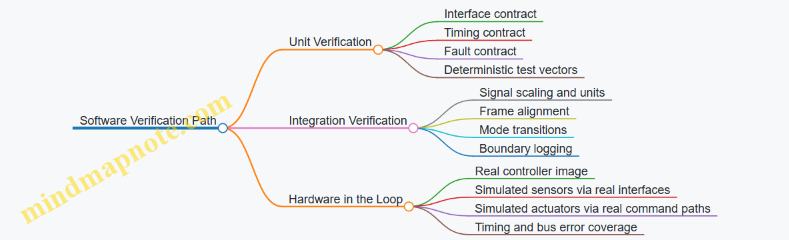
HIL Test Scenarios That Actually Break Things
Choose scenarios that stress the failure modes you care about.
-
Sensor dropout with recovery
- Inject IMU dropout for a defined interval.
- Confirm the controller enters a safe behavior and then returns to normal when data quality recovers.
-
Actuator saturation and rate limiting
- Command a thrust request beyond limits.
- Verify the controller respects saturation and does not produce unstable oscillations when the request returns to feasible values.
-
Timing jitter and missed deadlines
- Introduce controlled delays in sensor updates.
- Check that the scheduler and watchdog behavior matches your timing contract.
-
Bus and formatting errors
- Corrupt a packet or flip a bit in a simulated sensor message.
- Ensure the system detects invalid data and does not propagate nonsense into control outputs.
Example: If your actuator interface expects a specific command structure (e.g., thrust command plus enable flags), a HIL test should verify that disable conditions truly zero the command and that re-enable does not reuse stale values.
Evidence Collection and Acceptance Criteria
Verification isn’t complete until you can show repeatable evidence. For each test, record:
- Test ID, scenario parameters, and injected faults.
- Timing metrics: loop execution time, sensor-to-control latency, and missed deadline counts.
- Output metrics: thrust command bounds, attitude error response, and fault flags.
Set acceptance criteria per scenario. For instance:
- In sensor dropout, fault flags must assert within a specified number of control cycles.
- In saturation, the controller must keep commands within hardware limits and maintain bounded attitude error.
A Simple Example Test Matrix
Use a matrix to ensure coverage without turning every test into a novel.
| Layer | Scenario | What You Measure | Pass Condition |
|---|---|---|---|
| Unit | Filter step response | Settling time, overshoot | Within defined bounds |
| Integration | Axis alignment | Correlation of error to command | Correct sign and axis |
| HIL | Dropout recovery | Fault timing and safe output | Safe behavior then normal |
| HIL | Saturation | Command bounds and stability | No limit-cycle behavior |
Practical Mindset for Verification
Treat verification as a chain of responsibility. Unit tests prove each module honors its contract; integration tests prove the contracts still match when signals travel; HIL proves the real-time and I/O details don’t quietly break the assumptions. When something fails, the boundary logs and interface contracts make the root cause obvious instead of guessy.
9. Safety Engineering Including Fail Safe and Fault Tolerant Design
9.1 Defining Safety Requirements and Hazard Analysis Methodology
Safety requirements for a jet suit are not a checklist you hope will work; they are constraints that shape design decisions from the first block diagram to the last test card. The goal is to prevent unacceptable harm by identifying hazards, tracing them to specific safety requirements, and verifying those requirements with evidence.
Foundational Concepts and Safety Goals
Start by defining what “safe” means in measurable terms. For wearable propulsion, safety goals typically include preventing severe injury from thrust, heat, rotating components, loss of control, and unintended activation. Translate goals into system-level safety requirements such as:
- Maintain thrust and attitude within defined limits during normal operation.
- Detect and mitigate faults that could cause runaway thrust, loss of stabilization, or unsafe mode transitions.
- Ensure emergency shutdown actions are achievable by the pilot under realistic conditions.
A practical way to keep requirements grounded is to define harm categories and severity levels. For example, “loss of stabilization at low altitude” is more severe than “temporary sensor noise during cruise,” even if both are inconvenient.
Hazard Analysis Methodology Overview
Use a structured hazard analysis workflow that produces traceable outputs. A common approach combines:
- Hazard identification to list credible ways harm can occur.
- Hazard analysis to estimate severity and likelihood.
- Risk evaluation to decide what must be prevented or controlled.
- Safety requirement derivation to specify design and verification obligations.
- Verification planning to prove the controls work.
To avoid gaps, ensure every hazard has a clear chain: hazard → initiating cause(s) → hazardous event → potential harm → safety control(s) → verification method.
Mind Map: Hazard Analysis to Safety Requirements
Deriving Requirements from Hazards
Once hazards are identified, convert them into requirements that engineering teams can implement. Good safety requirements have these traits: they are testable, they specify boundaries, and they include timing where timing matters.
Example requirement patterns for jet suits:
- Thrust runaway prevention: If thrust command exceeds a safe envelope for longer than a specified time, the system must reduce thrust to a safe level and alert the pilot.
- Stabilization loss mitigation: If attitude estimation confidence drops below a threshold, the controller must switch to a conservative mode with reduced authority and clear pilot guidance.
- Unintended activation control: The system must require a deliberate arming sequence and must disarm automatically when arming conditions are not continuously satisfied.
Each requirement should link to a specific hazardous event. If multiple hazards share a control, document how the control addresses each hazard so verification does not become a guessing game.
Risk Evaluation Without Hand-Waving
Risk evaluation should be consistent. Define how you estimate likelihood using available evidence such as component failure rates, test coverage, and operational exposure. If you lack numerical data, use structured qualitative categories, but keep the mapping explicit.
A useful technique is to separate:
- Severity: how bad the outcome is.
- Exposure: how often the situation can occur.
- Controllability: whether the pilot can respond effectively.
For instance, a sensor dropout at high altitude might be less severe than at very low altitude because the pilot has more time and more room for recovery.
Example: Hazard to Requirement Trace
Hazardous event: Actuator stiction causes thrust response to lag the command during a rapid hover-to-cruise transition.
Potential harm: Loss of altitude control leading to hard landing or collision.
Safety controls:
- Detect thrust tracking error using commanded vs measured thrust.
- Limit commanded rate during transitions when tracking error grows.
- Provide an assisted recovery mode that reduces pilot workload.
Derived safety requirements:
- The system shall detect thrust tracking error exceeding a threshold within a defined time window.
- When detected, the system shall constrain transition commands to a safe profile and initiate assisted recovery.
- The system shall log the fault and mode transition for post-flight analysis.
This structure ensures the control is not just “there,” but measurable and verifiable.
Verification Planning as Part of Safety Requirements
Safety requirements are incomplete without verification. For each requirement, specify what evidence will demonstrate compliance. Typical evidence types include:
- Bench tests for thrust limiting and shutdown timing.
- Hardware in the loop for fault detection logic.
- Flight tests for pilot interface behavior and recovery procedures.
- Fault injection for sensor and actuator fault handling.
Verification should also confirm that safety controls do not introduce new hazards. For example, a shutdown that is too aggressive might cause a different loss-of-control scenario, so the verification plan must include boundary conditions.
Documentation and Traceability Discipline
Maintain traceability from safety goals to hazards to requirements to verification artifacts. A simple rule helps: if a requirement cannot be traced to a hazard, it probably belongs in a design note, not in the safety requirements set. If a hazard has no derived requirement, it means either the hazard is not credible or the analysis is incomplete.
A final practical touch: include a review checkpoint where human factors requirements are checked alongside technical ones. In wearable systems, “the controller works” is not the same as “the pilot can use it correctly under stress,” and safety requirements should reflect that reality.
9.2 Fault Detection for Sensor Dropout Actuator Stiction and Power Anomalies
Fault detection in a jet suit is mostly about being boring in the right ways: noticing when signals stop making sense, when actuators stop responding, or when power behavior changes. The goal is not to guess the exact cause; it is to classify the fault enough to choose a safe control action and a safe pilot experience.
Foundations for Detecting What “Wrong” Looks Like
Start with three layers of checks that build on each other.
- Signal plausibility: Does the sensor value stay within physical bounds and expected rates?
- Consistency: Do multiple measurements agree, or do they disagree in a repeatable pattern?
- Closed-loop behavior: When the controller commands something, does the system respond?
A practical example: if the inertial measurement unit (IMU) reports angular rate spikes, plausibility checks catch out-of-range values immediately. Consistency checks then verify whether accelerometer-derived attitude changes match the gyro trend. Finally, closed-loop checks confirm whether the attitude controller actually reduces the error. If only the sensor is wrong, control error may not behave as expected.
Sensor Dropout Detection
Sensor dropout means the data stream is missing, stale, saturated, or internally inconsistent.
Core checks
- Freshness timer: If a new sample does not arrive within a deadline, mark dropout.
- Staleness detection: If values repeat exactly for N cycles, treat as stale.
- Saturation and clipping: If the sensor reports max/min for longer than a threshold, treat as dropout-like.
- Rate-of-change limits: If the derivative exceeds what the vehicle can physically produce, flag the sensor as unreliable.
Example:
Suppose the IMU delivers gyro data at 200 Hz. The control loop runs at 100 Hz. If two consecutive control cycles see the same gyro timestamp, freshness fails. The system can then switch to a fallback estimator that relies more heavily on other sensors or holds the last known bias with increased uncertainty.
Decision logic
Use a fault state machine with hysteresis:
- Detect: trigger when checks fail.
- Confirm: require persistence for a short window to avoid reacting to one bad packet.
- Classify: label as “dropout” vs “out-of-range” vs “stale.”
Actuator Stiction Detection
Actuator stiction is when the commanded motion does not produce the expected change, often due to friction, sticking valves, or mechanical binding. The trick is to separate stiction from “the pilot asked for something impossible.”
Core checks
- Command-response mismatch: Compare commanded actuator position/thrust to measured actuator feedback.
- Error persistence: If control error remains high while commands stay within limits, suspect stiction.
- Unchanged actuator feedback: If actuator feedback stays flat despite changing commands, classify as stiction.
- Force/torque consistency: If thrust command changes but body acceleration does not follow the expected direction, stiction becomes more likely.
Example:
The controller commands a step increase in thrust for a hover correction. Actuator feedback (throttle valve position or thrust estimate) remains unchanged for 0.2 seconds while the command keeps moving. Meanwhile, body acceleration shows no corresponding response. This combination points to stiction rather than a sensor dropout.
Practical thresholds
Set thresholds using ground test data: measure typical response delay and steady-state tracking error. Then choose detection windows long enough to tolerate normal lag, but short enough to keep the pilot from feeling a “dead” control.
Power Anomaly Detection
Power anomalies include undervoltage, overcurrent, brownouts, regulator instability, and unexpected noise coupling into sensors.
Core checks
- Voltage and current limits: Detect undervoltage, overcurrent, and power rail dropouts.
- Power quality metrics: Watch for sudden changes in ripple or switching noise indicators.
- Correlation with sensor noise: If sensor noise increases at the same time as power rail instability, treat the sensor as indirectly affected.
- Compute health: If CPU load or ADC timing changes coincide with power events, suspect brownout behavior.
Example:
During a high-thrust maneuver, the power rail voltage dips below a threshold and the ADC readings show increased variance. The system should classify this as a power anomaly, then reduce thrust commands to regain stable power and prevent cascading faults.
Integrated Fault Classification and Safe Control Actions
Combine the three fault types into a single classification table that maps to control behavior.
- Sensor dropout: degrade estimation, increase uncertainty, and limit control aggressiveness.
- Actuator stiction: reduce commanded changes, avoid repeated oscillatory commands, and transition to a controlled recovery mode.
- Power anomaly: prioritize power stability, cap thrust/actuation rates, and prepare for shutdown if limits persist.
A simple rule that works well: when multiple faults occur, choose the action based on the most safety-critical one (usually power anomalies), but log all contributing evidence.
Mind Map: Fault Detection Evidence to Action
Example: End-to-End Detection Walkthrough
- The IMU freshness timer fails for two consecutive control cycles.
- Consistency checks show accelerometer-derived attitude still evolves smoothly.
- Closed-loop error does not behave like a true attitude disturbance.
- Classification becomes “sensor dropout,” not “stiction,” because actuator feedback tracks commands normally.
- The system switches to a fallback estimator and limits thrust command rate until fresh data returns.
This sequence keeps the system from overreacting while still taking action quickly enough to protect the pilot and the hardware.
9.3 Fail Safe Control Laws Including Safe Thrust Reduction and Shutdown
Fail-safe control laws define what the jet suit does when something goes wrong, without asking the pilot to guess. The goal is simple: keep the system predictable, reduce risk, and reach a known safe state using the least complicated actions that still work.
Foundational Concepts for Fail Safe Behavior
A fail-safe law starts with three building blocks.
- A trigger definition: what counts as a fault. Examples include sensor dropout, impossible attitude estimates, actuator command saturation for too long, or power rail undervoltage.
- A safe-state definition: what “safe” means for this platform. For a jet suit, safe typically means thrust reduced to a level that prevents runaway lift or unstable torque, followed by controlled shutdown when conditions allow.
- A transition policy: how the controller moves from normal control to safe control. This prevents step changes that can surprise the pilot or excite structural dynamics.
A practical rule is to separate control safety (stability and thrust limits) from system safety (valves, ignition, fuel flow, and power). The control law can keep the suit stable while the system safety layer performs the shutdown sequence.
Safe Thrust Reduction as the First Line of Defense
Safe thrust reduction is usually the fastest meaningful action. Instead of immediately commanding zero thrust, the controller reduces thrust authority in a controlled way.
Key elements:
- Thrust envelope: define a maximum allowable thrust command based on detected fault severity. For example, if attitude estimation is degraded but still bounded, allow only a reduced thrust ceiling.
- Rate limiting: cap how quickly thrust can change. If the suit normally ramps thrust at 20% per second, a fail-safe ramp might be 5% per second to avoid sudden pitch/roll moments.
- Authority reallocation: if differential thrust is used for attitude control, the controller should switch to a simpler allocation that avoids saturating one side. If one actuator is suspected, the law should bias toward the remaining healthy actuator while keeping total thrust within the safe envelope.
Example: Suppose the inertial measurement unit still provides angular rates, but the attitude estimate fails a consistency check. The fail-safe law can:
- reduce total thrust to 30–40% of nominal,
- hold the last known attitude target for a short time,
- then command a gradual descent profile by lowering thrust further once vertical motion remains within expected bounds.
Controlled Shutdown When Safe Reduction Is Not Enough
Shutdown is not just “turn everything off.” It is a sequence that respects actuator dynamics, fuel system behavior, and pilot safety.
A robust shutdown policy uses staged actions:
- Stabilize: apply safe thrust reduction and freeze or simplify guidance so the suit does not chase bad estimates.
- Confirm: verify that the fault persists and that sensors used for shutdown decisions are reliable. If the system can’t confirm, it should default to the most conservative safe thrust level.
- Actuate: command valves and ignition control to reach a no-thrust condition using known actuator timing.
- Verify: confirm thrust-related feedback or proxy signals indicate near-zero thrust before declaring shutdown complete.
Example: If a fuel valve position sensor reports “stuck open” while electrical current suggests normal operation, the law should not immediately cut power if that would create an unstable torque transient. Instead, it can reduce thrust authority, then command a valve close sequence with a conservative ramp, and finally verify closure using valve position feedback and engine response proxies.
Trigger Logic and Fault Severity Levels
Triggers should map to severity levels so the controller can choose the right response.
- Level 1: degraded sensing or minor inconsistency. Response: safe thrust reduction with continued stabilization.
- Level 2: loss of critical state estimate or actuator anomaly. Response: stronger thrust ceiling, simplified control, faster transition.
- Level 3: evidence of unsafe actuation, power anomalies, or multiple simultaneous faults. Response: immediate staged shutdown with minimal control complexity.
To avoid oscillation between levels, use hysteresis and minimum dwell times. If a fault clears briefly, the controller should not bounce between normal and fail-safe commands.
Mind Map: Fail Safe Control Laws
Implementation Pattern for Deterministic Behavior
A state machine keeps the behavior consistent and testable. Each state has explicit outputs and exit conditions.
Example state sequence: Normal → Safe Reduction → Shutdown → Shutdown Verified.
- Normal: full control with standard envelopes.
- Safe Reduction: thrust ceiling reduced, rate limits tightened, guidance simplified.
- Shutdown: valves commanded to close with a predefined timing profile.
- Shutdown Verified: controller holds outputs at no-thrust and waits for system reset.
The key is that the controller never relies on a single questionable signal to decide whether it is safe to keep flying. When confidence is low, the law chooses the conservative path.
Practical Example: Sensor Dropout to Verified Shutdown
Assume attitude estimate becomes unavailable due to sensor dropout.
- Trigger fires: Level 2 fault.
- Controller enters Safe Reduction: thrust ceiling lowered, attitude target frozen, thrust ramp slowed.
- If dropout persists beyond a dwell time and vertical motion proxies remain within safe bounds, controller transitions to Shutdown.
- Shutdown commands close valves using known actuator timing.
- Verification checks confirm near-zero thrust proxies; only then does the system declare shutdown complete.
This sequence keeps the suit stable long enough to reduce risk, then removes thrust in a controlled, verifiable way.
9.4 Emergency Procedures for Pilot Actions and System Responses
Emergency procedures are the bridge between “something is wrong” and “the system becomes safe again.” They work best when they are short, observable, and tied to specific cues the pilot can recognize without needing a perfect diagnosis.
Core Principles for Emergency Behavior
Start with three rules that keep decisions consistent under stress.
- Stabilize first, troubleshoot second. The pilot’s job is to reduce risk quickly, not to identify the exact fault. For example, if thrust response feels delayed, the immediate goal is to prevent aggressive control inputs that could saturate actuators.
- Use mode-aware actions. A hover emergency is not the same as a forward-flight emergency. Procedures should reference the current operating mode and the most likely control authority available in that mode.
- Make system responses predictable. The controller should follow a defined sequence when faults are detected, so the pilot can anticipate what will happen next.
Pilot Action Ladder
A practical emergency ladder uses escalating steps. Each step includes an action and a reason.
- Step 1: Reduce commands. Move inputs toward neutral and avoid rapid reversals. Example: if the suit pitches unexpectedly, keep stick movements small while centering them, because large inputs can fight the controller while it is trying to recover.
- Step 2: Select the safest available mode. If the interface provides a “safe hold” or “assisted recovery” switch, use it when the pilot can do so without losing orientation. Example: during a low-altitude wobble, assisted recovery can limit attitude excursions while thrust is managed.
- Step 3: Initiate controlled shutdown. If thrust authority is unstable or the system reports a critical fault, follow the shutdown procedure that reduces thrust in a controlled way rather than abruptly. Example: if actuator feedback disagrees with commanded thrust, a controlled thrust ramp-down prevents sudden changes in body loading.
- Step 4: Execute emergency landing posture. Use the posture and body alignment specified for the suit so the structure sees loads within design limits. Example: if the suit is descending, keep the torso aligned with the thrust vector to reduce lateral shear.
System Response Sequence
The controller’s emergency response should follow a consistent timeline: detect, confirm, transition, and stabilize.
- Detect. Fault detection checks include sensor plausibility, rate limits, and command-vs-feedback mismatch. Example: if IMU rates jump beyond expected bounds while the pilot inputs are neutral, the system flags an estimation fault.
- Confirm. Use short persistence windows to avoid reacting to brief glitches. Example: require mismatch to persist for 100–300 ms before triggering a thrust reduction.
- Transition. Enter a defined emergency state that changes control laws. Example: switch from full maneuvering control to a limited-authority stabilization controller.
- Stabilize. Apply safe thrust constraints and attitude limits. Example: cap thrust slew rate and clamp commanded attitude angles to reduce oscillations.
Emergency Triggers and What They Mean
Below are common triggers and the intended combined pilot-system response.
- Loss of attitude estimation: System limits attitude commands and relies on the best available sensors; pilot reduces inputs and uses assisted recovery if available.
- Thrust command/feedback mismatch: System ramps thrust toward a safe value; pilot avoids aggressive stick inputs and prepares for controlled descent.
- Actuator saturation or stiction: System reduces command gains and increases damping; pilot centers inputs and prioritizes stability over altitude changes.
- Power anomaly or undervoltage: System sheds nonessential loads and limits thrust; pilot transitions to the safest mode for the current phase.
Mind Map: Emergency Procedures Flow
Example: Hover Instability with Thrust Lag
Cue: The pilot commands a small increase in thrust, but the suit responds after a noticeable delay and then overshoots.
- Pilot Step 1: Center inputs and avoid repeated thrust taps.
- System Response: Detect command/feedback mismatch, confirm persistence, then enter a limited-authority stabilization state with reduced thrust slew rate.
- Pilot Step 2: If assisted recovery is available, engage it to hold attitude while the controller manages thrust.
- Pilot Step 3: If mismatch persists beyond the allowed window, initiate controlled shutdown and prepare for a controlled descent posture.
Example: Forward Flight with Estimation Dropout
Cue: Attitude cues become inconsistent; the suit’s response feels “off-axis” even with steady inputs.
- Pilot Step 1: Reduce commands and keep inputs smooth to avoid exciting oscillations.
- System Response: Clamp attitude commands and switch to the best available estimation path; limit lateral authority.
- Pilot Step 2: Select the safest mode for forward flight, typically one that prioritizes stable attitude and gradual deceleration.
- Pilot Step 3: If stabilization cannot be maintained, execute controlled shutdown and transition to the emergency landing posture.
Procedure Quality Checks
A procedure is usable when it meets three tests.
- Time-to-action: The pilot can perform the first step within a few seconds of recognizing the cue.
- Observability: The trigger can be confirmed by pilot-perceivable signals, not only by internal logs.
- Consistency: The system’s emergency state produces the same general behavior every time, so the pilot learns a reliable pattern rather than a one-off surprise.
9.5 Safety Validation Test Plans for Ground and Flight Conditions
Safety validation is where theory meets stubborn reality. A good test plan proves that hazards are controlled under both normal operation and the messy edge cases that show up when hardware, software, and humans all do their own thing.
Foundations for Safety Validation
Start by turning the safety requirements into testable claims. Each claim should map to a specific hazard control, such as “loss of attitude sensor triggers safe thrust reduction within 200 ms.” Then define measurable acceptance criteria: timing, thresholds, and allowable pilot workload.
A practical approach is to structure validation around three layers:
- Component and subsystem behavior (does the actuator respond as expected?)
- Integrated control behavior (does the control law react safely when inputs are wrong?)
- Operational behavior (does the pilot interface support correct recovery actions?)
Example: If the safety goal is “stuck actuator does not drive thrust beyond limits,” you first test actuator response with a bench load, then inject a simulated stuck command into the controller, then confirm the pilot can execute the emergency procedure without needing perfect timing.
Ground Test Plan Structure
Ground tests validate safety without the added complexity of flight dynamics. Use a staged progression so each step narrows uncertainty.
Stage A: Static checks
- Verify power rails, sensor health flags, and actuator command paths.
- Acceptance criteria: no unexpected resets; sensor fault flags assert within the specified detection window.
Stage B: Controlled actuation
- Command thrust and attitude-related actuators within conservative limits.
- Acceptance criteria: response time within bounds; no oscillation beyond defined tolerances.
Stage C: Fault injection in a safe environment
- Inject sensor dropout, bias shifts, and communication delays.
- Acceptance criteria: controller enters the intended safe mode; thrust is reduced to the defined safe envelope.
Stage D: Human factors verification on the ground
- Practice recovery procedures with realistic interface cues.
- Acceptance criteria: pilot can identify the fault mode and execute the correct action within a target time window.
Example: For a “sensor dropout” claim, run a repeatable sequence: normal operation for 10 seconds, then dropout for 2 seconds, then recovery. Log detection time, safe-mode entry time, and resulting thrust command profile.
Flight Test Plan Structure
Flight tests should be conservative, incremental, and tightly instrumented. Define a test matrix that varies only one major factor at a time: altitude band, thrust level, or maneuver type.
Flight test phases
- Phase 1: Low-risk envelopes such as tethered or near-ground hover with strict thrust caps.
- Phase 2: Expanded control authority with controlled maneuvers that stress the control allocation.
- Phase 3: Fault-mode demonstrations only after ground fault injection proves timing and safe thrust behavior.
Acceptance criteria examples
- Safe-mode entry within a specified time after fault detection.
- Thrust stays within the safe envelope for the entire fault duration.
- Pilot recovery action results in stable reversion to a safe operating mode.
A useful detail: define “stop conditions” that end the test immediately, such as unexpected oscillations, repeated watchdog resets, or inability to confirm mode transitions from logs.
Mind Map of Safety Validation Flow
Safety Validation Test Plans Mind Map
Example Test Case Templates
Example: Sensor Dropout Timing Test (Ground)
- Setup: controller running with simulated sensor input.
- Procedure: normal operation → dropout for 2 seconds → recovery.
- Checks: detection time, safe-mode entry time, thrust command envelope.
- Pass criteria: safe-mode entry within the defined window; thrust remains within safe limits.
Example: Actuator Stiction Recovery (Flight, Low-Risk Envelope)
- Setup: near-ground hover with conservative thrust cap.
- Procedure: induce stuck actuator behavior via controlled command path; observe safe-mode response; pilot executes recovery.
- Checks: stability during safe-mode; recovery action results in stable reversion.
- Pass criteria: no unsafe thrust excursions; pilot can complete recovery using the defined procedure.
Evidence Handling and Traceability
Validation is only as good as its evidence. Require that every test produces:
- raw logs (sensor, commands, mode flags)
- derived metrics (detection time, safe-mode entry time, thrust envelope compliance)
- a clear pass/fail statement tied to the specific safety claim
Keep a requirement-to-test trace so an auditor can follow the chain from hazard control to measured outcome. If a test fails, record the failure mode precisely—timing mismatch, threshold error, interface confusion—so the next iteration targets the real cause rather than guessing.
A simple rule: if you cannot explain why a test passed using the logged signals, the test is not finished yet, even if the pilot felt fine.
10. Power Systems Engineering for Wearable Propulsion
10.1 Power Source Selection Including Battery and Fuel System Constraints
Personal flight systems live or die by power availability under motion, heat, and safety constraints. Battery and fuel choices are not just about energy; they determine voltage stability, peak current capability, thermal headroom, packaging mass distribution, and how quickly the system can enter a safe state when something goes wrong.
Foundational Constraints That Drive the Choice
Start with the load profile. Jet suit propulsion typically demands short bursts of high power for spool-up, thrust transients, and control authority changes. A battery can supply high current, but only if its voltage sag stays within control electronics limits and the motor/actuator drivers can tolerate the resulting current. A fuel system can provide sustained energy, but it introduces constraints on fuel flow regulation, ignition/combustion stability, and thermal management of the power conversion path.
Next, define the “must-not-fail” boundaries. These include minimum bus voltage for flight control, maximum allowable battery temperature, maximum allowable fuel line temperature, and maximum acceptable rate of thrust reduction during a safety event. If your control system needs stable sensor readings, power ripple and ground noise become constraints too.
Finally, account for packaging and mass distribution. Batteries often sit near the harness center of mass to reduce pitch/roll coupling. Fuel tanks and regulators may be placed to minimize line length and heat soak into the suit structure. Either way, the placement affects wiring runs, connector choices, and the effectiveness of cooling.
Battery Systems and Their Practical Limits
Battery selection starts with chemistry and cell format, but engineering decisions usually hinge on three measurable behaviors: internal resistance, usable capacity under load, and thermal rise under repeated power cycles.
Internal resistance determines voltage sag during peak current. For example, if the controller requires at least 36 V at the bus and the battery is nominally 48 V, a high-resistance pack might dip below the threshold during thrust transients, causing resets or degraded control. Usable capacity under load matters because a pack that looks fine on a datasheet may deliver less energy when current is high and the pack is warm.
Thermal limits are often the real constraint. A battery that can deliver the required current at room temperature may exceed temperature limits after a few high-power segments. That means your mission profile must include worst-case duty cycles, not just total energy.
A simple example: suppose the suit needs 3 kW average during a hover segment and 10 kW peaks during transitions. If the battery can only sustain 6 kW continuous at the expected temperature rise, you must either reduce peak demand through control allocation limits, add buffering (like a supercapacitor stage), or accept shorter transition durations.
Fuel Systems and Their Practical Limits
Fuel systems shift the constraint from electrical sag to flow and combustion stability. Key parameters include fuel type energy density, regulator response time, line pressure stability, and how quickly the system can reduce thrust safely.
Regulation is the heart of fuel constraint management. If the regulator response is slow, the system may overshoot thrust commands during spool-up or undershoot during recovery. If the regulator is too aggressive, it can create oscillations that couple into vibration and sensor noise.
Thermal management matters because fuel can absorb heat, but it also warms regulators and lines. A line that runs hot can change viscosity and flow characteristics, which then changes thrust response. That’s why engineers often treat fuel temperature as a first-class variable, not an afterthought.
A concrete example: if the system requires a stable fuel flow rate to maintain consistent thrust, a regulator that drifts with temperature can cause thrust to vary even when commanded power is constant. The control system may try to correct, but it can only correct within actuator authority and sensor accuracy.
Constraint Mapping from Requirements to Hardware
Use a structured mapping so decisions don’t become “because it fits.”
- Power demand: average, peak, and transient rates
- Electrical limits: minimum bus voltage, allowable ripple/noise, connector current ratings
- Thermal limits: battery temperature rise, cooling effectiveness, hot-spot locations
- Safety limits: fault response time, safe thrust reduction behavior, isolation strategy
- Packaging limits: mass, center of mass shift, wiring length, service access
When you map these, you can compare battery-only, fuel-only, and hybrid architectures on the same axes: peak capability, thermal endurance, and safe shutdown behavior.
Mind Map: Power Source Selection Constraints and Decisions
Example: Choosing Between Battery-Only and Hybrid
Assume the suit must support repeated hover-to-transition cycles with short high-power bursts. If battery-only operation meets peak current and voltage sag limits at the expected temperature rise, it simplifies safety because electrical shutdown can be fast and deterministic. However, if the battery temperature limit is reached after a few cycles, you can either reduce peak demand through control allocation limits or add a buffering stage that handles transients while the battery handles sustained load.
If the mission requires longer sustained operation without exceeding thermal limits, a fuel system can provide energy without the same electrical thermal bottleneck. In that case, the engineering focus shifts to fuel regulation stability and safe thrust reduction. The control system must be designed so that when power drops due to a fault, the response is predictable and does not demand control authority beyond what the remaining power can deliver.
Practical Selection Checklist
- Verify peak current and transient voltage sag against the control bus minimum.
- Confirm thermal endurance using the actual duty cycle, not a single steady-state point.
- Validate fuel flow regulation response against thrust command dynamics.
- Ensure fault response time aligns with safe thrust reduction requirements.
- Check packaging impacts on cooling, wiring resistance, and connector ratings.
- Align control limits with the measured power capability so the controller never asks for the impossible.
10.2 Power Distribution Design for High Current Loads and Noise Control
High-current power distribution in a jet suit is less about “getting power there” and more about controlling where current returns, how voltage behaves under load steps, and how noise couples into sensors and control electronics. The goal is simple: the propulsion controller should see clean, predictable voltages while the pilot sees predictable behavior.
Foundational Principles for High Current Paths
Start by treating power as two coupled systems: the forward conductor and the return path. If you route the return poorly, the “noise” you fight later is often just current taking the shortest available path, not the intended one.
- Minimize loop area. For each high-current pair (supply and return), keep the physical loop small. A smaller loop reduces magnetic coupling into nearby signal wiring.
- Use a star or controlled return strategy. A star point at the power entry (or at a defined power module) prevents return currents from flowing through sensitive grounds.
- Separate power and signal grounds by intent. Join them at a single, well-defined node or through a controlled impedance strategy, so sensor references don’t ride on propulsion current spikes.
Example: If a motor driver draws 120 A peak and your return cable shares a thin ground trace with the IMU reference, the IMU ground can momentarily shift by tens of millivolts. That’s enough to look like angular motion to a filter.
Voltage Drop and Transient Behavior Under Load Steps
High-current loads rarely draw smoothly. Thrust changes, valve actuation, and pump start/stop create step-like current. Design for both steady-state drop and transient droop.
- Compute DC drop using conductor resistance and expected current. Keep it low enough that the controller’s undervoltage thresholds are not approached during normal maneuvers.
- Model transient droop using inductance and capacitance. Inductance dominates during fast edges; capacitance dominates right after the step.
Example: A wiring harness with 2 mΩ resistance is fine for DC, but if its effective inductance is high, a 1 ms current step can create a noticeable voltage dip at the controller input. Place local bulk capacitance near the load driver to reduce the dip at the electronics.
Noise Sources and Coupling Mechanisms
Noise comes from three main places: switching edges, current ripple, and ground impedance.
- Conducted noise travels along power rails and returns.
- Radiated noise couples through magnetic and electric fields, often from high di/dt loops.
- Common-mode noise appears when the entire system reference moves relative to chassis or environment.
The practical takeaway: you reduce noise by controlling current loops, adding filtering at the right location, and preventing sensitive circuits from sharing impedance with noisy currents.
Filtering Strategy That Actually Works
Filtering is not just “add a capacitor.” Use a layered approach with clear placement.
- Input protection and bulk energy storage. Use fusing and bulk capacitors to handle energy during transients.
- Local decoupling at the driver. Place high-frequency capacitors close to the switching device power pins.
- Rail filtering for electronics. Add LC or RC filtering for the control electronics rails so propulsion switching ripple doesn’t modulate sensor supply.
- Damping for resonances. Filters can ring. Add damping (often via ESR-aware capacitor selection or small series resistors) so the filter doesn’t amplify noise at a particular frequency.
Example: A common failure mode is placing an LC filter far from the electronics. The harness inductance forms an extra series element, shifting the filter’s behavior and letting switching ripple slip through.
Grounding and Return Path Discipline
Ground design is where many builds lose their battle.
- Define a single-point reference for sensor and controller grounds.
- Route high-current returns away from sensor ground reference routing.
- Use chassis bonding intentionally. If the chassis is used as a reference, bond it at controlled points so common-mode noise is managed rather than scattered.
Example: If you bolt the controller ground to the chassis at two locations, you create a ground loop. Under switching current, that loop can pick up magnetic flux and inject error into the sensor reference.
Connector, Harness, and Layout Rules
Physical layout is part of the electrical design.
- Twist or pair conductors for each high-current supply/return to reduce loop area.
- Route power and signal separately with a clear keep-out region.
- Avoid routing signal traces parallel to switching current paths over long distances.
- Use shielding where it helps, not where it looks good. Shield effectiveness depends on termination strategy.
Example: A shielded cable with the shield terminated at both ends can create a shield current path that increases common-mode noise. Terminate according to the grounding plan.
Measurement and Verification Plan
Noise control is validated by measurement, not hope.
- Measure at the load driver terminals for conducted noise and transient droop.
- Measure at the controller power input for what the electronics actually experience.
- Check ground offsets by probing between sensor ground and the defined reference node during load steps.
Example: If the controller input looks clean but the sensor ground shifts, the issue is ground impedance coupling, not rail filtering.
Mind Map: Power Distribution and Noise Control
Example: Practical Power Module Architecture
A robust architecture uses three zones: propulsion power zone, driver zone, and electronics zone.
- Propulsion power zone: bulk energy storage and fusing near the power entry.
- Driver zone: local decoupling and short, paired high-current loops to the switching devices.
- Electronics zone: filtered rails and a single defined ground reference node.
Example: During a thrust step, the driver zone absorbs the fast current edge using local capacitance, while the electronics zone sees a slower, filtered rail change. Your controller then receives stable supply voltage, and the IMU reference doesn’t jump when the propulsion current ramps.
Case Study: Diagnosing a Sensor Glitch During Thrust Changes
A pilot reports brief attitude estimate jumps during rapid thrust changes.
- Check controller input voltage during the event. If it dips, improve bulk and local decoupling near the driver.
- If controller input is stable, measure sensor ground offset relative to the defined reference node. If it shifts, reroute returns or change the ground join point.
- If both are stable, inspect loop area and routing parallelism. Switching current loops may be radiating into sensor wiring; pair and separate routes.
The fix is usually one of these: shorten the high-current loop, move the filter closer, or stop sharing impedance between propulsion current and sensor reference. That’s the whole game, repeated with different wiring and different numbers.
10.3 Thermal Management for Electronics and Power Conversion Units
Thermal management is the practical bridge between electrical power and safe, repeatable performance. In a jet suit, electronics sit in a cramped volume with limited airflow, while power conversion units (PCUs) must handle high currents and switching losses. The goal is not to “keep everything cold,” but to keep critical components within their allowable temperature and temperature-change rates, so control loops stay stable and reliability stays boring.
Start with Heat Sources and Thermal Paths
Begin by listing where heat is generated: power semiconductors (switching and conduction), magnetic components (core and copper losses), resistors (I²R), and any linear regulators or charge-management circuits. Then map where that heat can go: conduction into the frame, convection to any available airflow, and radiation to surrounding surfaces.
A useful rule of thumb is to treat the system as a chain of thermal resistances. If you know the worst-case power dissipation for each block, you can estimate junction temperature rise by summing resistances from junction to case to heatsink to structure to ambient. The “ambient” in a suit is not a single number; it changes with rider motion, clothing, and local airflow. So you size for the highest realistic local temperature and include margin for sensor and control electronics that may be near hot power stages.
Define Targets That Match Failure Modes
Set targets around the components that fail first or cause the most trouble. For example, power MOSFETs and IGBTs are sensitive to junction temperature, while electrolytic capacitors are sensitive to both temperature and ripple current heating. Control boards are sensitive to drift and intermittent faults caused by thermal cycling.
Instead of only limiting peak temperature, also limit temperature gradients. A steep gradient can warp PCBs, stress solder joints, and shift sensor readings. A practical target is to keep the hottest component-to-board temperature difference small enough that mechanical stress stays within your assembly limits.
Choose Cooling Strategy by Constraint
Most jet suit designs end up with a hybrid approach:
- Conduction-dominant: heatsinks or thermal spreaders bonded to the frame. This works well when airflow is limited.
- Convection-assisted: directed airflow paths created by suit motion or ducting, used to reduce the thermal resistance from heatsink to surrounding air.
- Radiation support: usually secondary, but helpful for surfaces that can “see” cooler surroundings.
Conduction is often the backbone. To make it effective, you need good contact: flat mating surfaces, appropriate thermal interface material (TIM), and controlled mounting pressure. TIM thickness and compression matter; too little pressure increases contact resistance, too much can pump out TIM or stress components.
Build a Thermal Model That Engineers Can Use
A first-pass model can be simple and still useful. Use a lumped thermal network for each major block and validate it with measurements. Measure surface temperatures on the heatsink and on the hottest PCB area during representative load profiles.
Example: Suppose a PCU dissipates 120 W at peak. If the thermal path from PCU case to frame has an effective resistance of 0.25 °C/W, the case-to-frame rise is 30 °C. If the frame surface near the PCU sits at 50 °C under worst conditions, the PCU case is around 80 °C. Then add junction-to-case resistance for the semiconductor to estimate junction temperature. This turns “it runs hot” into a number you can design around.
Manage Switching Losses and Ripple Heating
Thermal management is not only mechanical. Electrical choices reduce heat at the source.
- Switching frequency and gate drive: higher frequency can increase switching losses; gate drive shaping can reduce overlap losses.
- Conduction losses: lower resistance devices reduce I²R heating but may increase cost or switching behavior.
- Magnetics: core material choice and winding layout affect both copper and core losses.
A practical workflow is to compute loss breakdown at the operating points you actually expect, then compare thermal impact. If a design change reduces losses by 10 W, that can be the difference between “within spec” and “thermal throttling,” even if the heatsink size stays the same.
Use Thermal Monitoring Without Creating New Problems
Thermal sensors should be placed where they represent the risk, not where they are easiest to solder. For PCUs, measure heatsink temperature near the hottest device and, if possible, measure board temperature near sensitive components.
Also consider sensor self-heating and wiring heat conduction. Thin wires can act like thermal insulators, while thick conductors can steal heat from the measurement point. The sensor location should match the control action: if you throttle power based on heatsink temperature, the sensor must track heatsink temperature quickly enough to prevent runaway.
Design for Thermal Cycling and Serviceability
Thermal cycling causes fatigue. Use mechanical designs that tolerate expansion differences between components, TIM, heatsinks, and the frame. Avoid rigid constraints that force bending into the PCB.
Serviceability matters too. If a heatsink must be removed, ensure the mounting method preserves contact quality: repeatable fastener torque, consistent TIM replacement guidance, and alignment features that prevent rocking.
Mind Map: Thermal Management for Electronics and Power Conversion Units
Integrated Example: PCU with Heatsink and Sensor Feedback
Imagine a PCU mounted to a frame plate with a thermal spreader and TIM. You estimate worst-case semiconductor junction temperature using a thermal network, then confirm with a test that logs heatsink and board temperatures during a high-load run. If the heatsink sensor shows a slower rise than the semiconductor junction would imply, you adjust sensor placement or improve thermal coupling so the control action responds in time.
Finally, you verify that the mounting method is repeatable. A “works on the first assembly” design is not a thermal design; it’s a lucky one. Repeat the test after re-mounting to ensure the thermal resistance stays within your modeled range.
10.4 Energy Budgeting Including Duty Cycles and Efficiency Measurements
Energy budgeting answers a simple question: “How much useful work can the system do before the energy source runs out?” For jet suit systems, the tricky part is that “work” is not constant. Hover, climb, and maneuvering create different power profiles, and the pilot’s control inputs change the duty cycle.
Core Concepts for Energy Budgeting
Start with three quantities:
- Energy available: the total electrical or fuel energy the system can draw, after accounting for usable capacity.
- Power required: the instantaneous power needed for propulsion, control, and auxiliary loads.
- Efficiency: how much of the input energy becomes useful output (thrust, useful motion, or controlled attitude).
A practical budgeting workflow uses duty cycle to convert a variable power profile into an average power estimate.
Duty Cycles That Actually Matter
Duty cycle is the fraction of time spent in a particular operating state. For example, consider a mission segment broken into states:
- Hover hold: near-constant thrust with frequent small corrections.
- Acceleration: higher thrust demand for a short interval.
- Transition: changing thrust and control authority while maintaining stability.
- Idle/standby: electronics and sensors running, propulsion at minimum.
Compute average power as a weighted sum:
- Average power = Σ (state power × state time fraction)
Then estimate energy used as:
- Energy used = Average power × mission duration
If the system includes multiple energy domains (fuel-to-shaft, electrical-to-actuator, battery-to-compute), budget each domain separately and link them with measured efficiencies.
Efficiency Measurements That Don’t Lie
Efficiency depends on operating point. A single “overall efficiency” number is usually misleading, so measure efficiency in the same way you budget.
Use three measurement layers:
- Electrical efficiency for power electronics and motor/actuator drive
- Measure input electrical power and output mechanical or actuator power under representative loads.
- Propulsion efficiency for converting energy into thrust
- Measure thrust (or a validated proxy) and correlate it with fuel flow or shaft power.
- System efficiency for the full chain
- Measure total energy drawn from the source and compare it to a defined useful output metric (often thrust-weighted or maneuver-energy based).
A useful rule: if you can’t measure the output metric consistently, don’t pretend you can compute efficiency from thin air.
A Systematic Budgeting Example
Assume a 6-minute segment with these time fractions:
- Hover hold: 0.60 at 2.4 kW propulsion power
- Acceleration: 0.25 at 3.6 kW propulsion power
- Transition: 0.10 at 3.0 kW propulsion power
- Standby: 0.05 at 0.4 kW propulsion power
Auxiliary loads (controls, sensors, comms, cooling) are 0.25 kW during active states and 0.10 kW during standby.
- Average propulsion power:
- 2.4×0.60 + 3.6×0.25 + 3.0×0.10 + 0.4×0.05 = 2.61 kW
- Average auxiliary power:
- 0.25×(0.60+0.25+0.10) + 0.10×0.05 = 0.225 kW
- Average total power:
- 2.61 + 0.225 = 2.835 kW
- Energy used:
- 2.835 kW × 0.10 h = 0.2835 kWh
If the source provides 0.40 kWh usable, the energy margin is 0.40 − 0.2835 = 0.1165 kWh. That margin should also cover inefficiency changes due to temperature, component aging, and control aggressiveness.
Energy Budgeting Mind Map
Mind Map: Energy Budgeting
Duty Cycle Measurement in Practice
To measure duty cycle, log state indicators rather than trying to infer everything from raw power alone. For example, define state transitions using control mode flags and thrust command thresholds. Then compute time fractions from the logged timeline.
A clean approach is to separate steady-state from transients. If you include transients in the average, you must measure them consistently; otherwise, your budget will be optimistic during aggressive maneuvers.
Efficiency Measurement in Practice
When measuring efficiency, record the operating point alongside the measurement. At minimum, capture:
- thrust level or thrust command
- inlet conditions or cooling state
- battery voltage or fuel flow rate
- control mode
This lets you build an efficiency curve or a lookup table that matches the duty cycle states you defined. If your efficiency data only exists for one thrust level, your budget should only be trusted for that same region.
Final Budget Check
Before accepting a mission profile, verify that the budget is consistent across domains:
- Source energy used matches the sum of domain energy uses.
- Average power aligns with the measured power during representative tests.
- The margin is large enough to cover measured variability, not just measurement noise.
Energy budgeting is less about finding a perfect number and more about building a model that stays honest when the pilot changes the plan.
10.5 Electrical Protection Including Fusing Grounding and Surge Suppression
Electrical protection in a jet suit is less about “saving the day” and more about preventing small faults from turning into expensive smoke. This section ties three layers together: fusing for overcurrent, grounding for reference and fault return, and surge suppression for voltage spikes that slip past normal regulation.
Foundational Protection Goals and Failure Modes
Start by listing what can go wrong in the power path: short circuits, stalled loads drawing excess current, loose connectors creating intermittent arcs, and inductive kick from switching elements. Each failure mode suggests a different protection mechanism. A fuse is great for sustained overcurrent, grounding helps ensure faults clear predictably, and surge suppression handles brief overvoltage events that might not trip a fuse.
A practical rule: every protected circuit should have a defined “fault clearing path.” If a short occurs, current must rise enough to trigger the intended device, and the system must provide a safe return route so voltages don’t float to random values.
Fusing Strategy for Overcurrent Control
Fuses protect wiring and components by interrupting current before overheating. Choose fuse ratings using three checks: maximum continuous current, inrush or transient current, and fault current available from the source.
Example: Suppose a motor driver feeds an actuator that normally draws 8 A but can draw 20 A for 200 ms during spool-up. If the supply can deliver 200 A during a hard short, a fast-acting fuse rated too close to 8 A may nuisance-blow during spool-up. Instead, select a fuse whose time-current curve allows the 20 A transient while still clearing a sustained short.
Also decide where to place fuses. Common approaches include:
- Source-side main fuse to protect the entire harness.
- Branch fuses near loads to localize faults.
- Board-level protection for sensitive electronics where wiring is already protected.
Branch fusing is especially helpful for wearable systems because it limits the number of loads affected by a single connector failure.
Grounding for Fault Return and Stable References
Grounding is not just “connect to metal.” It defines how fault current returns and how measurement references stay consistent. In wearable propulsion, grounding must handle both safety and control reliability.
Key grounding practices:
- Single-point reference for sensitive electronics when feasible, so high current returns don’t inject noise into sensor references.
- Low-impedance fault return paths using appropriately sized conductors and reliable terminations.
- Mechanical integrity at ground straps and mounting points, because corrosion or paint can turn a “ground” into a “maybe.”
Example: If a sensor ground is tied to a chassis point that also carries actuator return current, the sensor may see voltage shifts during thrust changes. Even if the control loop still runs, the estimator can interpret those shifts as motion. Separating sensor ground returns or using a star topology reduces that coupling.
Surge Suppression for Switching and Inductive Events
Surges come from switching currents, inductive loads, and wiring inductance. They can exceed normal operating voltage briefly, stressing insulation and semiconductors without triggering a fuse.
Use suppression devices matched to the energy and waveform:
- TVS diodes across supply rails for fast clamping.
- RC snubbers or flyback paths for inductive elements.
- Proper wiring layout to reduce loop area, which lowers induced voltage.
Example: When a high-current valve driver turns off, the current through its coil must go somewhere. A flyback diode or controlled clamp limits the voltage spike at the driver pins. Without it, the spike can couple into the microcontroller supply and cause a reset, even though the average current never exceeded the fuse threshold.
Coordinating Protection Layers Without Surprises
Protection coordination means the fuse, grounding, and surge suppression work together rather than fighting each other.
- Ensure the surge clamp does not route current through sensor grounds. Route suppression currents to the power return path.
- Confirm the fuse clearing time is fast enough to prevent sustained heating in the faulted wiring.
- Verify that grounding provides a predictable return so fault current actually reaches the fuse.
Example: A branch fuse placed far from the load might not clear quickly if the fault return path is resistive. The voltage rise can stress insulation while the fuse waits for enough current to trip.
Mind Map of Electrical Protection Decisions
Mind Map: Electrical Protection for Jet Suit Power Paths
Practical Checklist for Implementation and Verification
- Identify every power path segment and list its maximum expected current and worst-case fault current.
- Choose fuse types using time-current behavior, not just nominal ratings.
- Define grounding topology: where power returns go, where sensor references connect, and how chassis bonds are made.
- Add surge suppression at the points where spikes enter the system: supply rails and inductive driver outputs.
- Validate with tests that reflect real wiring: measure voltage transients at the controller supply during switching and confirm fuses clear the intended faults.
This approach keeps protection deterministic: faults have a known path, spikes have a known clamp, and overcurrent has a known interrupter. The suit remains controllable even when the electrical environment is not perfectly polite.
11. Advanced Flight Technologies for Control Authority and Efficiency
11.1 Thrust Vectoring and Differential Thrust Allocation Strategies
Thrust vectoring changes the direction of produced thrust, while differential thrust allocation changes how much thrust each side produces. In a jet suit, both are usually constrained by actuator limits, sensor noise, and the pilot’s ability to perceive and correct motion. The goal is to create predictable control authority: when the pilot asks for a roll, pitch, or yaw change, the system should respond in a way that matches the control model and stays within mechanical and safety bounds.
Core Concepts and Control Mapping
Start with a simple mental model: the suit generates a net force and a net moment about the body. Net force affects translation, and net moment affects rotation. Vectoring primarily changes the moment by redirecting thrust forces; differential allocation primarily changes the moment by creating thrust imbalance.
A practical mapping is:
- Pitch control: vector thrust forward/backward or increase thrust on the appropriate side pair to create a pitching moment.
- Roll control: vector left/right or bias thrust between left and right to create a rolling moment.
- Yaw control: vector asymmetrically around the vertical axis or bias thrust to create a yawing moment, accounting for any coupling from the frame.
Because the pilot commands desired attitude changes, the controller produces desired moments. The allocator then converts desired moments into actuator commands, respecting limits like maximum gimbal angle, maximum thrust per nozzle, and minimum stable thrust.
Thrust Vectoring Mechanics
Vectoring can be implemented with gimbals, nozzle vanes, or differential exhaust direction. The key engineering detail is that vectoring changes both the direction and the effective lever arm of thrust. That means the same gimbal angle can produce different moments depending on suit geometry and thrust level.
A robust approach uses a control effectiveness model:
- Compute the thrust force magnitude from available power and fuel flow.
- Convert gimbal angles into a thrust direction in the body frame.
- Compute the moment as the cross product of position vector to the nozzle and the thrust vector.
Then the allocator solves for actuator settings that best match the requested moment. If the requested moment requires more vectoring than available, the allocator should reduce the moment demand in a controlled way rather than saturating one actuator and causing unexpected coupling.
Differential Thrust Allocation Mechanics
Differential allocation assumes thrust directions are fixed but magnitudes differ between actuators. This is often simpler mechanically, but it introduces coupling: changing thrust on one side can also change net force, not just moment.
To manage coupling, treat allocation as a constrained optimization problem:
- Decision variables: thrust commands for each actuator.
- Objective: minimize error between desired and achieved moments.
- Constraints: thrust bounds, rate limits, and any required minimum thrust to keep the system stable.
A common simplification is to allocate moments first and then compensate net force with a separate loop, but that only works if the force-to-moment coupling is small. In jet suits, it can be noticeable, so the allocator should include both moment and force terms when possible.
Unified Allocation Strategy
Vectoring and differential thrust can be combined. A unified allocator uses both actuator types to achieve the same moment request with better margin. For example, use differential thrust for coarse moment generation and vectoring for fine correction near hover, where small attitude changes matter.
A systematic workflow:
- Compute desired wrench: desired moments (and optionally desired force).
- Predict actuator effectiveness: moment contribution per actuator at the current thrust level.
- Solve allocation with constraints: choose actuator commands that meet limits.
- Apply rate limiting and smoothing: prevent abrupt changes that the pilot will feel as “laggy” or “twitchy.”
- Validate with saturation logic: if constraints bind, adjust the commanded wrench so the achieved response matches the control model.
Mind Map: Allocation with Vectoring and Differential Thrust
Example: Roll Command Near Hover
Assume the pilot requests a positive roll moment. The controller outputs a desired roll moment \( M_x \). The allocator considers two options:
- Differential thrust only: increase left thrust and decrease right thrust. This creates \( M_x \) but also changes net vertical force, which can cause a small altitude drift.
- Vectoring assist: apply a small vector angle on both sides to create \( M_x \) while keeping thrust magnitudes closer to the hover value.
A good allocator will prefer the second option when altitude stability is critical. It does this by including a force term in the objective, such as minimizing moment error while penalizing net force deviation from the hover target.
Example: Yaw Command with Asymmetric Limits
Suppose the right-side vectoring actuator is near its gimbal limit due to a prior maneuver. A naive allocator might still demand the same yaw moment, forcing the remaining actuators to saturate and producing unexpected roll coupling.
A constrained allocator instead detects that the effectiveness matrix is constrained and reduces the demanded yaw moment to what the remaining actuators can produce. It then updates the attitude controller’s expected response so the pilot sees consistent behavior: the suit turns as much as it can, without surprising side effects.
Practical Implementation Notes
Effectiveness models must be updated with current thrust level and estimated nozzle direction. Rate limiting should be applied to actuator commands, not directly to the desired moments, because the allocator needs to know what it can actually achieve. Finally, log the achieved moments and net force during tests; if the achieved response consistently lags or overshoots in a specific axis, the allocation weights or effectiveness parameters likely need adjustment.
11.2 Attitude Estimation Using Sensor Fusion and Bias Handling
Attitude estimation answers a simple question: “Where is the suit pointing, and how fast is it turning?” In a jet suit, that answer must be stable enough for control loops, fast enough for pilot inputs, and honest enough to fail safely when sensors misbehave. The core challenge is that sensors measure different things with different errors. Gyros measure angular rate but drift; accelerometers measure gravity direction but get confused by acceleration; magnetometers measure heading but get disturbed by nearby metal and current.
Foundations of Sensor Fusion for Attitude
A practical attitude estimator typically combines:
- Gyroscope: provides short-term rotation rate, excellent for smooth control.
- Accelerometer: provides a gravity reference, good for long-term leveling when linear acceleration is small.
- Magnetometer: provides a magnetic heading reference, useful for yaw but sensitive to interference.
The estimator maintains an internal state that includes orientation and sensor biases. Bias handling matters because even a small gyro bias can accumulate into a noticeable attitude error within seconds.
Bias Handling That Actually Helps
Gyro Bias as a First-Class State
Model the measured angular rate as:
- Measured rate = True rate + Bias + Noise
If you ignore bias, the filter will “explain away” the mismatch by changing attitude, which then fights the accelerometer and magnetometer. Treating bias as a state lets the estimator slowly adjust bias estimates when the other sensors provide reliable reference.
A useful rule of thumb: bias should change slowly compared to attitude. That means your bias dynamics should be low bandwidth, so the estimator doesn’t chase momentary disturbances.
Accelerometer Bias and Scale
Accelerometers can have offset and scale errors. Offsets can mimic gravity errors, especially when the suit is nearly level. Scale errors distort the inferred gravity direction. In practice, you can reduce these effects by calibration and by trusting accelerometer direction only when the suit’s linear acceleration is small.
Magnetometer Bias and Distortion
Magnetometer errors are often not just bias but distortion: the field is warped by the suit’s structure and electronics. Bias handling here means two things: calibration to correct hard-iron effects, and careful weighting so magnetometer influence drops when interference is likely.
A Systematic Estimation Workflow
Step 1: Calibrate and Validate Sensor Outputs
Before fusion, ensure each sensor stream is consistent:
- Check gyro bias at rest by averaging several seconds of stationary data.
- Verify accelerometer magnitude near 1 g when stationary.
- Verify magnetometer readings form a reasonable sphere or ellipse after calibration.
If any sensor fails these checks, the estimator will spend its time compensating for problems you could have fixed earlier.
Step 2: Choose a Reference Frame and Orientation Representation
Use a consistent frame convention for control and estimation. Many systems use quaternions internally to avoid singularities. The estimator outputs orientation and angular rate estimates aligned with the control law.
Step 3: Fuse with Measurement Gating
Not all measurements are equally trustworthy at all times.
- Accelerometer gating: trust gravity direction only when the measured acceleration magnitude is close to 1 g and when changes are smooth.
- Magnetometer gating: reduce yaw correction when magnetic field magnitude deviates from expected values or when the suit is near high-current components.
Gating prevents the estimator from “learning” the suit’s maneuvers as if they were gravity.
Step 4: Update Bias Estimates Using Residuals
Residuals are the differences between predicted sensor outputs and actual measurements. When residuals persist, the filter can attribute them to bias rather than attitude error. This is where bias handling becomes more than a modeling detail.
Step 5: Maintain Consistency Through Covariance Tuning
Covariance tuning controls how quickly the estimator reacts. If gyro noise is set too low, the filter will over-trust gyro and ignore reference sensors. If set too high, attitude will jitter as it chases accelerometer noise.
Mind Map: Attitude Estimation with Sensor Fusion and Bias Handling
Example: Hover with Turning and Linear Acceleration
Imagine the suit hovers and the pilot initiates a yaw turn while also making a small forward push. The gyro will track the yaw rate immediately, but the accelerometer will see extra forward acceleration, so its gravity direction estimate becomes less reliable.
A well-behaved estimator will:
- Continue using gyro prediction for attitude during the push.
- Gate accelerometer updates when acceleration magnitude deviates from 1 g.
- Allow magnetometer yaw correction only if magnetic magnitude and residuals look normal.
- Adjust gyro bias slowly if residuals show a consistent offset during periods where gating permits reference updates.
The result is a roll and pitch estimate that stays stable during the push, and a yaw estimate that converges without “rubber-banding” to every acceleration blip.
Example: Sensor Dropout and Bias Recovery
Suppose the magnetometer signal becomes noisy for a few seconds. The estimator should reduce magnetometer weight to near zero, relying on gyro integration for yaw. During that time, gyro bias still gets updated indirectly through other constraints when available, but yaw will drift slowly because there is no absolute reference. When magnetometer quality returns, the estimator should reintroduce yaw corrections smoothly rather than snapping, which is achieved by covariance and gating logic.
Bias handling is what prevents the estimator from permanently baking in the dropout period’s errors into attitude. Instead, it treats the missing reference as a temporary loss of observability and resumes correction when measurements become trustworthy again.
11.3 Disturbance Estimation and Compensation for Ground Effect and Gusts
Ground effect and gusts both show up as “the air is doing something different than expected,” but they differ in how they behave. Ground effect is strongly tied to height and geometry, while gusts are more about time-varying wind and turbulence. A good disturbance estimator treats them separately, then blends their compensation so the controller doesn’t fight itself.
Foundational Model of Disturbances
Start with a simple plant view: the controller commands thrust allocation and attitude targets, but the vehicle experiences additional forces and moments. Represent the disturbance as an additive term in the translational and rotational dynamics. For practical engineering, you don’t need a perfect physics model; you need a model that explains the dominant patterns.
For ground effect, the dominant pattern is height-dependent lift augmentation and altered drag. For a jet suit, this often appears as a bias in vertical acceleration and a coupling into pitch/roll when the thrust line and body attitude are not perfectly aligned.
For gusts, the dominant pattern is a time-varying external force that projects into the body axes. The same gust can look like a vertical disturbance when the body is pitched, so the estimator should work in a consistent frame.
Height-Based Ground Effect Estimation
Ground effect compensation begins with a height estimate. Use the best available altitude source, then filter it to avoid injecting sensor noise into the disturbance estimate. The estimator can use a parametric form such as a gain that increases as height decreases, saturating at very low heights.
A concrete approach:
- Compute a normalized height ratio h/Href.
- Map it through a smooth curve to produce an estimated vertical force bias ΔFz.
- Convert ΔFz into an equivalent thrust or acceleration correction using the current mass and thrust-to-acceleration relationship.
Example: if the suit is hovering at a height where the estimator predicts +8% effective lift, the controller will observe less thrust needed to maintain the same vertical acceleration. Instead of waiting for integral action to “figure it out,” you apply a feedforward correction that reduces the thrust command by the predicted amount.
Gust Estimation Using Residuals
Gusts are harder because they are not tied to a single measured variable like height. A reliable method is residual-based estimation: compare measured motion to what your controller model predicts.
Steps:
- Predict body acceleration (or angular acceleration) from commanded thrust and attitude dynamics.
- Compute residuals: r = measured − predicted.
- Filter residuals to separate persistent disturbances from noise.
- Project residuals into disturbance forces/moments using the inverse of your control effectiveness mapping.
Example: during a lateral gust, the estimator sees a roll-rate residual that cannot be explained by the commanded differential thrust. It converts that residual into an estimated roll moment disturbance, then adjusts the control allocation to counter it.
Sensor Fusion and Frame Consistency
Disturbance estimation fails when frames don’t match. Ensure that:
- Residuals are computed in the same frame as the disturbance model.
- Any gravity compensation uses the same attitude estimate used by the controller.
- Height-based ground effect uses the same reference point as the altitude sensor.
A practical trick: log the residual components in body axes and also in inertial axes. If the estimator is correct, the inertial residual should show gust-driven patterns, while the body residual should show how those gusts couple through attitude.
Compensation Blending and Authority Limits
Ground effect and gusts can overlap. If you add both compensation terms directly, you may exceed actuator limits or create oscillations. Blend them with a weighting strategy:
- Use ground-effect weight that increases as height decreases.
- Use gust weight that increases when residual energy rises and height-dependent prediction is insufficient.
Then enforce authority limits:
- Clamp the estimated disturbance correction to what the actuators can counter.
- Rate-limit changes in the disturbance estimate to avoid “chasing” noise.
Example: at very low height, the ground-effect estimator might be confident, but gust residuals can still appear due to imperfect thrust alignment. Clamping prevents the gust estimator from overriding the height-based correction when the suit is already near its thrust authority boundary.
Mind Map: Disturbance Estimation and Compensation
Validation Through Targeted Tests
Validate estimation quality by checking what changes when you enable compensation.
- With ground-effect compensation enabled, steady hover thrust should show less bias across a height sweep.
- With gust compensation enabled, the controller should require smaller corrective effort, visible as reduced residual magnitude and smoother actuator commands.
Example test logic: hold attitude commands constant, then introduce controlled lateral disturbances (e.g., airflow) while logging residuals. If the estimator is working, the roll-rate residual should drop, and the commanded differential thrust should become less “bursty.”
Practical Implementation Notes
Keep the estimator modular: one block for height-based ground effect and one for residual-based gusts. Use consistent filtering across both so the combined disturbance estimate doesn’t introduce phase lag that the controller can’t tolerate. Finally, treat the estimator output as a correction term with bounds, not as a truth source—because the air rarely reads the spec sheet.
11.4 Control Allocation Under Asymmetric Thrust and Component Limits
Control allocation is the step where the controller’s desired forces and moments get converted into actuator commands that the jet suit can actually produce. The key complication in this section is asymmetry: one side may generate less thrust, a nozzle may respond slower, or a component may hit a limit earlier than the rest. Allocation turns those realities into predictable behavior rather than “whatever happens.”
Core Idea from Commands to Actuators
Start with a desired wrench vector, typically
- desired roll moment \(M_x\)
- desired pitch moment \(M_y\)
- desired yaw moment \(M_z\)
- desired collective thrust \(T\)
Then map it to actuator thrusts \(t_1, t_2, \dots\) through an effectiveness model \(B\): \[ \begin{bmatrix}T \\ M_x \\ M_y \\ M_z \end{bmatrix} = B,\begin{bmatrix}t_1 \\ t_2 \\ t_3 \\ t_4\end{bmatrix} \] In an ideal world, \(B\) is constant and invertible. In a jet suit, \(B\) changes with mounting flex, nozzle wear, and sensor-estimated thrust effectiveness. Allocation therefore uses a constrained solver that respects actuator limits and accounts for the current \(B\).
Constraints That Actually Matter
Actuator limits are not just “min and max thrust.” They include:
- Saturation: \(t_i \in [t_{i,min}, t_{i,max}]\)
- Rate limits: \(\dot{t_i}\) limited by spool/valve dynamics
- Deadband and stiction: small commands may not move the actuator
- Asymmetric capability: one actuator has a smaller \(t_{i,max}\) or a worse \(\dot{t_i}\)
A practical allocation approach treats these as hard constraints and uses the best achievable wrench under those constraints.
A Systematic Allocation Procedure
- Compute the desired wrench from the outer-loop controller and human input mapping.
- Update effectiveness \(B\) using the latest thrust/attitude data and actuator health indicators.
- Form the constrained optimization: choose \(t_i\) to minimize wrench error while satisfying limits.
- Apply rate limiting to prevent command jumps that the hardware can’t follow.
- Validate authority by checking whether the requested moments are feasible; if not, reduce the achievable wrench in a controlled way.
A simple mental model helps: allocation is like trying to hit a target with four springs that have different maximum stretches and different speeds. You can still aim, but you must accept that some directions are harder than others.
Handling Asymmetric Thrust with Weighted Allocation
When one actuator is weaker, a naive least-squares solution will overuse it and then clip, causing moment errors and oscillations. Weighted allocation fixes this by penalizing the use of constrained actuators more strongly.
For example, suppose actuator 4 has \(t_{4,max}\) reduced by 30% due to a partial blockage. The allocator should:
- still use actuator 4 if it helps reduce yaw moment error
- avoid saturating actuator 4 when the same moment can be produced by actuators 1–3 with acceptable efficiency
This is achieved by incorporating actuator-specific weights into the objective function, so the solver prefers thrust distributions that match both the physics and the limits.
Example: Yaw Command with One Weak Actuator
Assume a four-actuator layout where yaw moment \(M_z\) depends on differential thrust between left and right sides. The pilot requests a positive yaw moment while maintaining a fixed collective thrust \(T\).
- Desired: \(T=200,N\), \(M_z=+20,N\cdot m\)
- Actuator 2 is degraded: \(t_{2,max}\) is 60% of nominal
A feasible allocation might:
- keep the collective thrust near 200 N by distributing the remaining thrust across actuators 1, 3, and 4
- produce as much of \(M_z\) as possible using the available differential authority
- if \(M_z\) cannot reach +20 \(N\cdot m\) without violating \(t_2\) limits, the allocator returns the closest achievable \(M_z\) and the controller learns to avoid asking for the impossible in the next cycle
The important detail is that the allocator’s output is consistent with the constraints, so the outer-loop sees a predictable mapping from command to response.
Mind Map: Control Allocation Under Asymmetry and Limits
Practical Notes for Implementation
Use the allocator output to compute the achieved wrench and feed it back to the controller or estimator. This closes the loop on authority loss: if the allocator can’t meet \(M_y\) due to asymmetric limits, the controller should not keep integrating error as if nothing changed.
Also, keep the effectiveness model \(B\) aligned with how thrust is measured or estimated. If thrust feedback is biased, allocation will “correct” the wrong thing and saturate the wrong actuator. In other words: allocation is only as honest as the model it trusts.
11.5 Performance Evaluation Metrics Including Stability Tracking and Energy Use
Performance evaluation for a jet suit is mostly about two things: whether the suit stays where the control system thinks it should, and how much energy it spends to do that. The trick is choosing metrics that can be computed from logged data, interpreted by humans, and tied back to design decisions.
Stability Tracking Metrics That Actually Matter
Start with a clear definition of “tracking.” In practice, you will compare a commanded state (what the controller asked for) with an estimated or measured state (what the suit actually did). Use metrics that separate steady behavior from transient behavior.
1) Attitude tracking error
- Metric: root-mean-square (RMS) error of roll, pitch, and yaw angle over a defined phase.
- Example: During hover, if commanded pitch is 0° and measured pitch hovers around 1.5° RMS, you likely have a consistent bias or calibration offset.
2) Rate tracking error
- Metric: RMS error of body rates (p, q, r) or rate command tracking.
- Example: If attitude error is small but rate error is large, the controller may be “late” and correcting only after the suit drifts.
3) Settling time and overshoot
- Metric: time to enter and remain within a tolerance band after a step in command.
- Example: Command a small pitch step during a controlled test. If it overshoots by 8° and takes 2.5 s to settle within ±2°, you can trace the behavior to loop gains or actuator limits.
4) Stability margin proxies
- Metric: frequency-domain gain/phase margins are ideal, but for suit logs you often use time-domain proxies like oscillation frequency and damping ratio estimated from response.
- Example: If the suit shows a repeating “wobble” at a consistent period, you can correlate it with sensor filtering, structural modes, or control allocation saturation.
5) Human-relevant stability
- Metric: pilot workload proxy from control effort and mode switching counts.
- Example: If the pilot repeatedly toggles assist modes or uses large input corrections to keep the suit level, tracking might look acceptable in raw error metrics but still feel unstable.
Energy Use Metrics That Separate Waste from Necessity
Energy metrics should reflect both total consumption and how efficiently the suit converts energy into useful motion.
1) Total energy per phase
- Metric: integral of electrical power draw over time, reported per phase (hover, transition, low-speed cruise).
- Example: If hover consumes 120 Wh for a 6-minute session, you can compare hover efficiency across controller revisions.
2) Thrust-to-power efficiency
- Metric: average thrust magnitude (or net vertical thrust component) divided by average power.
- Example: Two controllers might both maintain altitude, but one achieves it with lower average thrust, indicating better disturbance rejection or better feedforward.
3) Control effort energy
- Metric: energy associated with actuator commands, not just total system power. Use actuator power estimates or command magnitudes mapped to expected electrical load.
- Example: If total power is high while thrust efficiency is low, the suit may be fighting oscillations or compensating for sensor noise.
4) Peak power and thermal stress
- Metric: maximum power and time-above-threshold values.
- Example: A controller with slightly better tracking might still be unacceptable if it repeatedly triggers thermal limits due to aggressive corrections.
5) Energy per unit of task
- Metric: Wh per meter of horizontal displacement or Wh per meter of climb, depending on the test.
- Example: If two cruise controllers cover the same distance, the one with lower Wh/m is the better baseline for operational planning.
Mind Map: Stability Tracking and Energy Use Metrics
Example: Turning Logs Into Comparable Metrics
Use a consistent test phase window, such as the 20 s interval after hover command stabilization. Compute stability metrics from commanded vs measured states, and compute energy metrics from power logs over the same window.
Example workflow:
- Segment the log into hover, transition, and cruise using mode flags.
- For hover, compute RMS roll/pitch error and rate error.
- Compute settling time after the first small step command.
- Integrate electrical power to get Wh for the same 20 s window.
- Report thrust-to-power efficiency using average net vertical thrust divided by average power.
If controller A has slightly worse attitude RMS but better thrust-to-power efficiency and lower control-effort energy, it may be the more stable-feeling option because it spends less energy correcting noise and oscillations.
Example: Interpreting Conflicting Metrics
A common outcome is “good tracking but high energy” or “moderate tracking but low energy.”
- Good tracking, high energy: likely aggressive actuator behavior, poor feedforward, or oscillation damping that costs power.
- Moderate tracking, low energy: possibly conservative control gains or insufficient disturbance rejection, which may still be acceptable if pilot workload stays low.
The evaluation is complete only when stability and energy are interpreted together, not separately, because the suit’s control choices trade precision, authority, and energy in the same physical loop.
12. Integration Testing and Operational Validation for Jet Suit Systems
12.1 Ground Test Procedures Including Bench Spin and Static Thrust Checks
Ground testing earns its keep by answering three questions before anyone straps in: does the propulsion hardware produce the commanded thrust, does the control system behave predictably, and do the mechanical interfaces survive the loads they will see. This section lays out a systematic path from bench spin fundamentals to static thrust verification, with examples you can adapt to your own jet suit test rig.
Test Objectives and What “Good” Looks Like
Start by writing measurable acceptance criteria for each test step. For bench spin, “good” usually means stable sensor readings, no unexpected oscillations, and repeatable actuator response. For static thrust, “good” means thrust magnitude matches the expected range, thrust rise time is consistent, and the system reaches commanded setpoints without runaway behavior.
Example acceptance criteria:
- Bench spin: attitude estimate drift stays within a defined band over a fixed duration (for example, 30–60 seconds), and commanded actuator positions track within a tolerance.
- Static thrust: thrust settles within a tolerance band after a defined ramp time, and thrust noise stays below a threshold during steady state.
Bench Spin Test Setup and Safety Checks
A bench spin test isolates rotational dynamics and control response without the full flight environment. Mount the propulsion module and frame in a rigid test fixture that constrains unintended translation. Install sensors where they will be in the real system: same mounting points, same cable routing, and the same harness strain relief.
Before powering anything, do a “no-energy” inspection:
- Verify fastener torque marks and thread engagement.
- Confirm that wiring harnesses cannot chafe under vibration.
- Confirm that emergency power cut access is unobstructed.
Example: If your test fixture uses a gimbal or pivot, label the axes and record the axis mapping used by your control software. A wrong axis mapping is the most common reason a controller “works” on paper and misbehaves on the stand.
Bench Spin Test Procedure from Baseline to Stress
Use a staged approach so you can attribute anomalies to specific causes.
-
Baseline sensor check
- Log raw IMU and any rate sensors while the system is stationary.
- Confirm bias stability and absence of saturation.
-
Low-power spin
- Command a small thrust or actuator output that produces measurable rotation.
- Run for a short duration and verify that the controller reaches and holds the target.
-
Incremental stress steps
- Increase command in steps, keeping each step short enough to avoid overheating.
- After each step, review logs for overshoot, oscillation growth, and actuator saturation.
-
Recovery and shutdown verification
- Confirm that the system returns to a safe state when commands drop to zero.
- Verify that watchdog or health monitoring triggers behave as expected.
Example: If you see a growing oscillation at higher command levels, check whether the actuator is hitting rate limits or whether sensor filtering is introducing phase lag. Bench spin is ideal for separating control-loop issues from structural issues.
Static Thrust Check Setup and Calibration
Static thrust checks quantify thrust output against commanded values. Use a thrust stand with a load cell or calibrated force measurement system. Rigidly connect the propulsion unit to the stand so that force is transmitted through the intended path.
Calibration steps should be explicit:
- Zero the load cell with the system at operating temperature if your setup warms significantly.
- Verify linearity by applying known weights or calibration forces.
- Record the measurement chain: load cell model, amplifier settings, sampling rate, and any filtering.
Example: If your load cell is sensitive to side loads, add alignment features so the thrust vector stays centered. A small misalignment can create a force component that looks like thrust variation.
Static Thrust Test Execution with Controlled Ramps
Static thrust tests should use repeatable command profiles.
-
Preheat and stabilization
- Run a low-level command to reach thermal stability.
- Confirm that thrust readings are stable before starting the main sequence.
-
Ramp to setpoints
- Use a defined ramp rate to each thrust setpoint.
- Hold each setpoint long enough to measure steady-state thrust.
-
Step down and repeat
- Step down to zero and repeat the sequence at least twice.
- Compare runs to assess repeatability.
-
Record and analyze
- Compute rise time, steady-state error, and noise level.
- Check for hysteresis by comparing ramp-up and ramp-down results.
Example: If thrust rise time increases with repeated runs, you may be seeing thermal effects in valves or control electronics. Static thrust checks are the right place to quantify that behavior.
Data Review Checklist and Common Failure Modes
Review logs with a consistent checklist:
- Command vs measured thrust alignment in time.
- Actuator command saturation events.
- Sensor health flags and any filtering changes.
- Temperature and power supply stability.
- Structural vibration indicators if available.
Common failure modes to watch for:
- Load cell saturation or drift.
- Control loop instability that only appears at higher command.
- Mechanical looseness that changes thrust transmission.
- Misconfigured sampling rates that make rise time measurements misleading.
Mind Map: Ground Test Flow
Example: A Minimal Test Card for Bench Spin and Static Thrust
Use a short, repeatable sequence so you can compare results across hardware revisions.
-
Bench spin
- 10 seconds baseline logging
- 20 seconds low-power spin hold
- 20 seconds medium-power spin hold
- 10 seconds shutdown and recovery logging
-
Static thrust
- thermal stabilization at low command for a fixed duration
- ramp to setpoint A, hold, ramp to setpoint B, hold
- step down to zero and repeat once
Record the exact command values, ramp rates, and hold times. If a result changes, you want the difference to be explainable rather than mysterious.
12.2 Hardware in the Loop and Closed Loop Validation Steps
Hardware in the Loop (HIL) and closed loop validation are where you stop arguing with models and start testing the real interfaces: sensors, actuators, power electronics, timing, and safety logic. The goal is not to “prove flight,” but to prove that the system behaves correctly under controlled, repeatable conditions.
Foundational Setup and Interfaces
Start by locking down the signal contract between controller, plant interface, and safety monitor.
- Define I/O maps: list every signal with units, scaling, update rate, and expected ranges. Example: IMU gyro in deg/s at 500 Hz, thrust command in percent at 200 Hz.
- Match timing: confirm controller loop period, sensor sampling, and actuator command latency. Example: if the controller assumes 5 ms actuation delay but HIL uses 2 ms, you will tune gains for the wrong world.
- Calibrate signal conditioning: verify offsets and gains for sensor emulation. Example: if barometer emulation outputs altitude with a 0.8 m bias, your altitude-hold mode will “hunt” even when the plant is stable.
HIL Architecture and Test Harness
A practical HIL setup separates concerns so failures are diagnosable.
- Plant emulator: provides vehicle dynamics outputs (attitude rates, altitude, thrust response) based on commanded inputs.
- Actuator and power interface: models motor/valve dynamics and electrical limits, including saturation and rate limits.
- Safety monitor: runs the same fault detection and safe-state logic as in the real system.
Mind the boring parts: clock synchronization, deterministic scheduling, and consistent units. If you can’t reproduce a failure twice, you can’t fix it.
Closed Loop Validation Steps
Proceed in layers, increasing realism only after each layer passes.
-
Open-loop interface checks
- Command each actuator channel with fixed inputs and verify the controller outputs match expected waveforms.
- Example: send a step thrust command and confirm the actuator interface reports the correct ramp rate and saturates at the configured limit.
-
Sensor-to-estimator consistency
- Feed static and slowly varying sensor scenarios and verify state estimation tracks without drift.
- Example: hold “level” attitude for 30 seconds; the estimated roll/pitch should remain within a tight bound and bias estimates should converge.
-
Inner loop stability under nominal plant
- Validate rate control or attitude control using the plant emulator with conservative dynamics.
- Example: apply a small commanded yaw rate; check overshoot, settling time, and that control effort stays below actuator limits.
-
Outer loop tracking with disturbance injection
- Add controlled disturbances such as thrust lag, ground-effect-like lift changes, or sensor noise bursts.
- Example: inject a 10% thrust gain error for 2 seconds; the controller should correct without oscillation and should return to baseline.
-
Mode transitions and state machine correctness
- Exercise every transition path: idle to hover-ready, hover-ready to hover, hover to landing, and abort paths.
- Example: trigger an abort during hover; verify thrust ramps down using the safe law and that the system refuses to re-enter hover until conditions reset.
-
Fault injection and fault-to-action mapping
- Confirm that each detected fault leads to the correct response.
- Example: simulate IMU dropout; the estimator should flag the fault, the controller should switch to a safe control mode, and the safety monitor should log the event.
-
Timing stress and CPU load tests
- Introduce worst-case scheduling conditions to ensure deadlines are met.
- Example: run with maximum telemetry and logging enabled; verify missed deadlines do not cause unstable control outputs.
Mind Map: Validation Workflow
Evidence, Metrics, and Pass Criteria
Define acceptance criteria before running tests.
- Stability metrics: overshoot, settling time, steady-state error, and oscillation frequency.
- Limit compliance: actuator saturation duration, command rate limits, and thermal/power constraints.
- Safety behavior: time-to-safe-state after each fault, and correct mode lockout behavior.
Example: for a hover-ready to hover transition, require thrust command to reach target within a specified time window, attitude error to remain bounded, and any fault during transition to force a controlled ramp-down.
Practical Example Test Card
- Scenario: level hover with a brief thrust gain error.
- Steps: start in hover-ready, transition to hover, inject gain error for 2 seconds, then remove it.
- Checks: attitude error stays within bounds, thrust command does not chatter at saturation, estimator remains consistent, and logs show a single fault-free run.
When these steps pass, you have strong evidence that the controller, interfaces, and safety logic work together in a closed loop—without needing a real flight to find basic integration mistakes.
12.3 Flight Test Planning Including Test Cards and Acceptance Criteria
Flight test planning turns “we think it will work” into “we can prove it worked for the conditions we tested.” The core idea is to plan in layers: define the test objective, choose the scenario, specify the instrumentation and procedures, then write acceptance criteria that map to measurable outcomes. If the criteria are vague, the test card becomes a checklist with no teeth.
Foundational Test Card Structure
A test card is a single, self-contained plan for one scenario. It should fit on one page, but still include enough detail to run without improvising.
Key fields to include:
- Objective: What behavior is being verified (e.g., hover stability under a specific thrust command profile).
- Initial Conditions: Pilot state, suit configuration, sensor health status, and environmental assumptions.
- Scenario Steps: A numbered procedure with explicit control inputs and timing.
- Data Requirements: Which signals must be recorded and at what rate.
- Safety Constraints: Abort triggers and maximum allowable excursions.
- Acceptance Criteria: Pass/fail rules expressed as thresholds and timing windows.
A practical example: If the objective is “mode transition safety,” the scenario steps should include the exact sequence of mode changes, and the acceptance criteria should specify what must happen during the transition window.
Acceptance Criteria That Actually Decide Pass or Fail
Acceptance criteria should be written in terms of observable signals and clear time windows. Use three categories so you don’t mix “it felt fine” with “it met the spec.”
- Performance: Stability tracking, attitude error bounds, altitude hold error bounds.
- Robustness: Behavior under sensor dropout, actuator saturation, or small disturbances.
- Safety: Limits on thrust rate, attitude rate, structural load proxies, and emergency triggers.
Example acceptance criteria for a hover test:
- Attitude error: Roll and pitch absolute error ≤ 3° for the final 10 s of the hover segment.
- Altitude hold: Vertical position error within ±0.5 m for the final 10 s.
- Control authority: No sustained actuator saturation longer than 2 s.
- Safety: Abort if vertical speed exceeds 2 m/s or if commanded thrust rate exceeds the defined limit.
Notice the criteria are measurable and time-bounded. Without time windows, you can “pass” by having a brief spike that you forgot to notice.
Systematic Test Planning Flow
Start with a minimal set of scenarios that establish baseline behavior, then expand coverage.
- Baseline Validation: Confirm sensor alignment, estimator stability, and controller response in calm conditions.
- Envelope Expansion: Increase thrust levels, then expand attitude commands while staying within safety constraints.
- Coupling Checks: Verify how human inputs interact with the control allocation and assist modes.
- Fault and Recovery: Trigger controlled faults (e.g., simulated sensor dropout) and verify safe degradation.
- Integration Stress: Combine higher workload inputs with realistic timing and transitions.
Each step should reuse the same acceptance criteria framework, adjusting thresholds only when the test objective changes.
Mind Map: Flight Test Cards and Criteria
Example Test Card Snippet with Acceptance Criteria
Test Card ID: HVR-01
Objective: Verify hover stability and mode-hold behavior at nominal thrust.
Initial Conditions:
- Sensor health: estimator valid, no fault flags.
- Pilot: standardized stance and input posture.
- Environment: calm air, defined temperature range.
Scenario Steps:
- Arm system and confirm logs.
- Climb to target altitude using assisted takeoff.
- Enter hover-hold mode and hold for 20 s.
- Apply a small step in pilot input and return to neutral.
Acceptance Criteria:
- Attitude error ≤ 3° for the final 10 s of hover.
- Altitude error within ±0.5 m for the final 10 s.
- After the small input step, attitude settles within 2 s and remains within bounds for the next 5 s.
- No actuator saturation longer than 2 s.
- Abort if vertical speed exceeds 2 m/s or if any safety limit is exceeded.
Data Review Checklist Tied to Criteria
After the flight, review in the same order as the criteria. Confirm signal integrity first, then compute metrics within the specified time windows.
A simple rule: if a required signal is missing or corrupted during the acceptance window, the result is “inconclusive,” not “pass.” That keeps the test program honest and prevents accidental acceptance of bad data.
For repeatability, require at least two runs for each new configuration before tightening thresholds. The goal is not to collect more flights; it’s to ensure the criteria reflect consistent behavior rather than one lucky pass.
12.4 Data Review Workflows for Controller Tuning and Safety Verification
A good data review workflow turns “we flew it” into “we can explain why it behaved that way.” The goal is not to find one magic plot; it’s to connect controller behavior, pilot inputs, sensor quality, and safety protections into a traceable story.
Data Set Definition and Review Readiness
Start by labeling each run with the minimum context needed to interpret it: test phase (hover, transition, cruise, landing), controller mode, configuration version, and any safety events (thrust limiting, mode changes, watchdog resets). Then verify data completeness: timestamps aligned across IMU, actuator commands, thrust estimates, and pilot input channels.
A practical rule: if you cannot reproduce the exact signals used for tuning, you cannot claim the tuning is responsible for the observed improvement. For example, if actuator command logs are missing for one motor, you may still see attitude oscillations, but you cannot tell whether the controller saturated or the plant failed to follow.
Signal Triage Before Tuning
Before touching gains, sort signals into three buckets.
- Reference and intent: pilot input commands, mode flags, setpoints.
- Measured state: attitude estimate, rates, altitude/position, sensor health flags.
- Actuation and constraints: thrust commands, actuator feedback, saturation indicators, limiter outputs.
If sensor health flags show dropout or bias jumps, treat the run as a measurement-quality problem first. Example: a sudden yaw rate spike that coincides with gyro bias correction usually means the estimator is reacting, not the controller “going unstable.”
Controller Behavior Decomposition
Once signals are clean, break the response into components that map to controller structure.
- Tracking error: difference between commanded and estimated attitude/rates.
- Control effort: actuator command magnitude and rate of change.
- Limiter interaction: when and how often thrust or rate limits engage.
- Closed-loop stability indicators: oscillation frequency, damping trend, and phase lag.
Example workflow for a hover test: if tracking error grows while control effort hits a thrust limiter, the issue is authority, not tuning. If tracking error shrinks but oscillations persist, the issue is likely damping or estimator latency.
Safety Verification Evidence Collection
Safety verification should be evidence-based and specific. For each run, record whether the system met safety criteria such as:
- Fault detection correctness: did the system flag sensor dropout when it occurred, and did it avoid false positives during normal motion?
- Fail-safe response: when a simulated fault or induced anomaly occurs, did thrust reduction follow the expected sequence and timing?
- Constraint compliance: did the controller respect hard limits for thrust, command slew, and attitude bounds?
Example: during a controlled sensor dropout test, confirm that the estimator falls back to a safe mode, that control effort decreases within the defined window, and that pilot inputs do not override safety limits.
Tuning Loop with Acceptance Metrics
Use a repeatable loop: hypothesis → targeted change → run set → metric check → decision.
Hypothesis examples
- “Increase damping to reduce oscillation amplitude without increasing steady-state error.”
- “Reduce estimator lag impact by adjusting filter bandwidth or fusion weights.”
Acceptance metrics
- Peak tracking error during step inputs.
- Settling time within a tolerance band.
- Control effort smoothness measured by command slew rate.
- Number of limiter engagements per minute of flight.
- Safety event correctness rate.
Example: if raising damping reduces overshoot but increases steady-state error, you likely need a compensator balance change rather than only damping gain.
Review Artifacts and Decision Records
Every tuning decision should produce a short record: what changed, which runs were used, which metrics improved, and which risks increased. Keep it boring and consistent.
A useful template for each run:
- Run ID and mode
- Key plots reviewed (tracking, control effort, limiter flags, sensor health)
- Safety checks passed/failed
- Metric deltas versus baseline
- Final decision: accept, re-run, or reject
Mind Map: Data Review Workflow for Controller Tuning and Safety Verification
Example Run Review Walkthrough
Consider a hover run where attitude oscillations appear after a small pilot step.
- Triage: sensor health shows no dropout; estimator bias correction is stable.
- Decomposition: tracking error oscillates with a period matching the controller’s inner-loop response; control effort also oscillates, suggesting closed-loop resonance rather than actuator lag.
- Limiter check: thrust limiter engages briefly at the first peak, then releases; that indicates authority is tight but not the root cause.
- Safety evidence: no fault flags, no watchdog resets, and command slew stays within the configured bound.
- Decision: adjust damping-related gains and re-run the same step input set, comparing peak error and settling time.
This approach keeps the review systematic: you do not guess. You classify the behavior, verify safety constraints, then tune the part of the controller that matches the observed mechanism.
12.5 Maintenance Procedures Including Inspection Intervals and Component Replacement Criteria
Maintenance for personal flight systems is mostly about staying ahead of wear, loosening, and sensor drift—before they show up as “mysterious” control behavior. A good procedure is systematic: inspect what changes, measure what matters, and replace based on evidence rather than vibes.
Maintenance Foundations for Jet Suit Hardware
Start with a clear maintenance baseline for each subsystem: propulsion units, fuel/power delivery, structural frame and harness, sensors and wiring, and the flight computer/control actuators. For every item, define three things: what failure mode it can contribute to, what inspection can reveal early, and what replacement threshold ends its service life.
A practical interval strategy uses three layers:
- Time-based: catches predictable aging like seals and fasteners.
- Usage-based: catches wear proportional to duty cycle like bearings and valves.
- Condition-based: catches drift or damage indicated by measurements like vibration signatures or sensor bias.
Example: if a thrust valve shows increasing actuation current over repeated flights, you don’t wait for the calendar interval. You treat it as condition-based replacement.
Inspection Intervals That Match Wear Mechanisms
Use a tiered schedule so routine checks stay short and deeper inspections happen when they’re most informative.
- Pre-Flight Inspection (quick, pilot-accessible): verify harness integrity, visible wiring condition, connector seating, and that the system reports no active faults. Example: tug-test the main sensor connector by hand; if it moves more than a small amount, reseat and inspect the strain relief.
- Post-Flight Inspection (short, technician): check for fastener loosening, abnormal residue, and any signs of heat stress near power electronics. Example: look for discoloration around cable glands; it often correlates with poor sealing or airflow blockage.
- Scheduled Service Interval (planned, deeper): perform functional checks, sensor calibration verification, and structural inspection of load paths. Example: run a controlled hover test profile and compare attitude hold error to the last service baseline.
- Major Overhaul Interval (full teardown scope): replace wear items with known service life limits and inspect internal components that are hard to assess without disassembly.
A common mistake is using only time-based intervals. If your duty cycle varies, usage-based triggers prevent unnecessary replacements and reduce risk.
Component Replacement Criteria Based on Measurable Thresholds
Replacement criteria should be written as thresholds tied to measurable indicators. Use “replace if any criterion is met” logic.
Key categories and examples:
- Fasteners and Attachment Hardware: replace if torque-mark evidence shows movement after re-torque, if threads are stripped, or if corrosion pits exceed a defined size. Example: if a locknut loses its prevailing torque after two re-torques, replace the nut and inspect the mating threads.
- Seals and Gaskets: replace if leakage indicators appear, if compression set exceeds a limit during inspection, or if heat exposure shows hardening. Example: if a fuel-line seal shows cracking at the lip after repeated thermal cycles, replace the seal set rather than only the visible part.
- Valves and Actuators: replace if actuation current rises beyond a threshold, if response time increases, or if position feedback deviates from command beyond tolerance. Example: if valve travel time increases by more than a specified percentage compared to the service baseline, schedule replacement.
- Sensors and Wiring: replace if bias drift exceeds calibration tolerance, if noise increases beyond the expected band, or if insulation damage is found. Example: if IMU bias requires repeated recalibration to pass acceptance tests, replace the sensor module.
- Structural Components: replace if cracks are detected, if deformation exceeds allowable limits, or if fatigue indicators appear in high-load regions. Example: if a harness attachment plate shows fretting marks that correlate with increased play during inspection, replace the plate and inspect the underlying load path.
Acceptance Tests That Confirm Replacement Was the Right Call
After replacement, run a verification sequence that proves the system is back within limits.
- Calibration Verification: confirm sensor bias and scale factors match acceptance ranges.
- Functional Checks: verify actuator response, fault detection behavior, and mode transitions.
- Control Performance Checks: compare stability metrics like attitude hold error and control effort to the pre-defined baseline.
Example: after replacing a thrust valve, you should see both improved response time and restored feedback tracking, not just “no faults.”
Mind Map: Maintenance Planning and Decision Making
Practical Example Workflow with Clear Decisions
On 2026-04-01, a technician performs a scheduled service after a higher-than-usual number of flights. The inspection finds increased valve actuation current and slightly slower response time compared to the last baseline. The procedure triggers condition-based replacement for the valve assembly, followed by calibration verification and a hover test profile. The system passes acceptance when both feedback tracking and stability metrics return to within tolerance.
This workflow matters because it ties the decision to evidence, then confirms the result with tests that reflect how the system actually behaves.