Orbital Manufacturing Platforms
1. Scope and Definitions for Orbital Manufacturing Platforms
1.1 Defining Orbital Manufacturing Platforms and Their Functional Boundaries
An orbital manufacturing platform is a space-based system that turns raw inputs into manufactured outputs using controlled processes, with the ability to manage energy, materials, quality, and operations while operating in an orbital environment. The key word is platform: it includes not only the tools that shape material, but also the interfaces that keep everything working as a coherent production system.
A useful way to define boundaries is to separate the platform into production functions and support functions. Production functions transform inputs into outputs. Support functions keep the production functions stable, safe, and measurable.
Production Functions
Production functions include:
- Process execution: running the manufacturing steps such as printing, machining, joining, coating, or curing.
- Workpiece handling: positioning parts for each step, including transfer between stations.
- In-process control: monitoring critical variables like temperature, power, feed rate, layer geometry, or cure time.
- Inspection hooks: capturing measurement data at defined checkpoints so quality is not guessed at the end.
Example: In an orbital additive workflow, the platform boundary covers the printer motion system, the feedstock delivery path, the deposition monitoring sensors, and the post-deposition handling that moves the part to heat treatment.
Support Functions
Support functions include:
- Power and energy management: distributing power to tools, heaters, lasers, pumps, and control electronics.
- Thermal management: removing heat from electronics and processes, and maintaining process temperatures.
- Vacuum and contamination control: managing outgassing risk, particulate containment, and cleaning steps.
- Data and control: running the manufacturing execution logic, logging parameters, and coordinating tool states.
- Materials logistics: storing consumables, tracking lot identity, and moving items to where processes need them.
- Safety and fault handling: interlocks, emergency shutdown paths, and recovery procedures.
Example: If a platform uses a powder-based process, the boundary includes containment hardware and filtration paths that prevent powder from migrating into sensitive avionics.
Functional Boundaries as Interfaces
Boundaries are easiest to manage when expressed as interfaces. A platform must clearly state what it accepts and what it delivers.
- Input interfaces: material forms (powder, wire, blanks, substrates), tooling consumables, and required documentation such as lot traceability.
- Output interfaces: finished parts, intermediate assemblies, scrap streams, and measurement packages.
- Operational interfaces: command and telemetry channels, crew or robotic access points, and maintenance access.
A practical rule: if a component is required for the platform to produce a conforming item, it belongs inside the boundary. If it only enables transport to or from the platform, it belongs outside.
Mind Map: Platform Scope and Boundary Decisions
Boundary Examples That Avoid Common Confusions
- Tool vs. station: A laser head is a tool, but the boundary includes the station that aligns the beam path, manages shielding, and verifies calibration status.
- Measurement vs. metrology system: A single sensor is not the whole boundary; the boundary includes calibration routines, reference artifacts, and data handling needed to interpret measurements.
- Consumables vs. logistics: A curing lamp is a tool, but the boundary includes the storage, handling, and tracking that ensure the correct lamp settings and consumable identity are used.
A Simple Boundary Checklist
Use this checklist to decide what is inside the platform:
- Can the platform produce a conforming item without external intervention during a defined run?
- Are quality-critical variables measured and logged within the platform boundary?
- Are safety interlocks and fault recovery actions implemented where the risk occurs?
- Are material identity and process parameter traceability maintained from input to output?
If the answer is “yes” for a function, it belongs in the boundary. If the answer is “no,” the platform definition is incomplete, and the missing piece will show up later as a quality or operational failure mode.
1.2 Mapping Industrial Processes to Orbital Constraints
Industrial processes work on assumptions: gravity helps chips fall, convection moves heat, and air carries away fumes. Orbital manufacturing breaks those assumptions, so the mapping step is about making the hidden assumptions visible and then replacing them with orbital-safe equivalents.
Foundational Step: Write the Process as a Constraint-Driven Workflow
Start by expressing each process as a sequence of unit operations with inputs, outputs, and control variables. For each unit operation, list what must be true for quality to hold. Then attach the orbital constraints that can violate those truths.
A practical way to do this is to create a “unit operation card” for each step. Each card should include:
- Primary function (what quality characteristic it creates)
- Key inputs (materials, energy, environment)
- Key controls (temperature, power, feed rate, dwell time, alignment)
- Failure modes (what goes wrong and how it shows up)
- Orbital sensitivity (which constraint most directly affects it)
Example: For a laser additive step, the primary function is layer geometry. Key controls include laser power, scan speed, and powder feed rate. A failure mode is poor fusion causing porosity. Orbital sensitivity is mainly related to powder behavior and heat dissipation.
Orbital Constraint Categories and What They Break
Map constraints to the process assumptions they disrupt. Use a consistent set of categories so teams don’t invent new vocabularies mid-project.
- Microgravity and particulate behavior break assumptions about settling, drainage, and debris removal.
- Vacuum and outgassing break assumptions about atmosphere-supported reactions and stable material chemistry.
- Thermal environment breaks assumptions about convection cooling and uniform heat removal.
- Radiation and charging can affect sensors, electronics, and some materials.
- Mechanical disturbance and station keeping can affect alignment, tool paths, and metrology.
- Mass and volume limits constrain storage, containment, and tool layouts.
- Power and data bandwidth limit process duty cycles and real-time monitoring.
The mapping goal is not to list everything; it is to identify which constraints directly threaten the quality characteristic for each unit operation.
Constraint-to-Process Mapping Method
Use a matrix approach: for each unit operation, ask “Which constraint changes the governing physics?” and “What control variable compensates?”
A simple rule helps: if the process relies on a physical mechanism that changes in orbit, you must either (a) redesign the mechanism, (b) add containment or handling, or (c) change the process parameters and acceptance criteria.
Example: In microgravity, molten metal does not drain the same way. If a process assumes gravity-assisted pooling, you can redesign the workholding and add controlled surface tension management, or switch to a process variant that does not depend on drainage.
Mind Map: Mapping Industrial Processes to Orbital Constraints
Worked Example: From Process Steps to Constraint Controls
Consider a simplified “machining then inspection” workflow for a precision bracket.
-
Blank preparation: The blank must be clean and dimensionally stable.
- Constraint mapping: vacuum can change surface contamination behavior; thermal cycling can warp thin sections.
- Control strategy: specify cleaning steps that do not rely on solvent evaporation in air, and define a thermal conditioning step before machining.
-
CNC machining: The tool path must match the part geometry.
- Constraint mapping: microgravity affects chip evacuation; vibration from station keeping can degrade surface finish.
- Control strategy: use chip containment and controlled evacuation, then define a vibration-aware machining window and toolpath compensation based on measured reference features.
-
Metrology inspection: The measurement must be traceable.
- Constraint mapping: sensor calibration can drift under radiation and thermal gradients.
- Control strategy: schedule calibration checks tied to the same thermal state as the inspection, and record environmental readings alongside measurement results.
Each step ends with a verification hook: what test or observation confirms the constraint mitigation worked.
Advanced Detail: Turning Mapping into Engineering Decisions
Once the mapping is complete, convert it into three engineering artifacts.
- Constraint-Process Matrix: a table-like structure that links each unit operation to the top constraints and the chosen compensations.
- Control Strategy Notes: a short list of which variables are actively controlled versus which are passively managed.
- Verification Plan Hooks: for each mitigation, define how you will prove it during qualification and production.
Example: If chip evacuation is mitigated by containment, the verification hook is not “it looks clean.” It is a measurable criterion such as chip accumulation limits, surface roughness targets, and post-process inspection of critical faces.
Common Mapping Pitfalls
Teams often stumble when they treat constraints as global facts rather than step-specific influences. Another frequent issue is mixing “what could happen” with “what will break quality.” The mapping should stay tied to quality characteristics and control variables, so the result is actionable rather than a long list of concerns.
1.3 Distinguishing Payload Manufacturing From In Orbit Servicing and Assembly
Payload manufacturing and in orbit servicing and assembly (IOSA) both happen in space, but they answer different questions. Payload manufacturing produces an item that must meet a defined performance specification at delivery. IOSA modifies, repairs, or combines existing hardware to restore function, extend life, or complete a mission configuration. The difference matters because it drives requirements, tooling, quality gates, and how you prove “it works.”
Core Definitions and What They Imply
Payload manufacturing starts with raw materials or components and ends with a finished payload ready for integration. The process plan typically includes controlled material inputs, repeatable process parameters, and inspection that verifies the item against acceptance criteria.
IOSA starts with hardware already in orbit or already qualified for flight. The work focuses on interfaces, alignment, and functional restoration. Instead of proving the entire manufacturing chain, you prove that the modification or repair meets interface and performance requirements without breaking existing constraints.
A simple way to remember it: payload manufacturing is about building from the ground up; IOSA is about changing what is already there.
Requirements and Quality Gates
Payload manufacturing quality gates are usually end-to-end. You track lot or batch information, confirm process settings, and measure critical dimensions or material properties. If a part fails, the failure is treated as a manufacturing nonconformance.
IOSA quality gates are more interface and outcome oriented. You verify that the servicing action correctly mates to the target hardware, that seals or bonds meet functional requirements, and that the repaired or assembled system passes verification tests. If something fails, the failure is often treated as an integration or execution nonconformance.
Example: If you print a structural bracket in orbit, you validate geometry, surface finish, and material properties before it ever touches the payload. If you replace a worn bracket on an existing satellite, you validate the new bracket’s fit, attachment quality, and the resulting system performance, while also ensuring you did not damage surrounding components.
Tooling and Workcell Design
Payload manufacturing workcells emphasize process stability and repeatability. Tooling is designed to control inputs like feedstock, energy delivery, and thermal profiles. Workholding must support consistent geometry, and metrology must be integrated enough to close the loop on dimensional accuracy.
IOSA workcells emphasize reach, compliance, and safe interaction. Tooling often includes docking adapters, alignment aids, capture mechanisms, and containment features to manage debris and contamination during contact. The workcell must handle uncertainty: the target may be tumbling, surfaces may be aged, and access paths may be constrained.
Example: A machining station for payload manufacturing can assume a known fixture position and stable reference frames. A servicing tool must compensate for variable approach angles and must still deliver the correct torque, weld energy, or adhesive cure conditions at the interface.
Data, Traceability, and Evidence
Payload manufacturing traceability is typically extensive because the item’s performance depends on the manufacturing history. You record material identifiers, process parameters, inspection results, and calibration status of measurement equipment.
IOSA traceability is still important, but the evidence focus shifts. You record target identification, docking and alignment logs, tool settings used during the operation, and verification outcomes such as leak checks, electrical continuity, or functional test results.
A practical example: For a payload cable harness manufactured in orbit, you track wire lot, termination process parameters, and insulation resistance measurements. For an IOSA cable replacement, you track the connector mating sequence, the tool calibration used for crimping or soldering, and the post-install electrical checks.
Operational Flow and Failure Modes
Payload manufacturing follows a production flow: receive inputs, process, inspect, rework if allowed, and release. Rework is planned because the item is under your control.
IOSA follows an execution flow: approach, capture, configure, perform the operation, verify, and release. Rework is limited because the target hardware is already operational or constrained by mission timelines.
Example: If a printed part shows a dimensional deviation, you may reprint or machine it. If a servicing operation misaligns a connector, you may not have the option to “start over” without risking collateral damage or losing access.
Mind Map: How to Tell Them Apart
Integrated Decision Checklist
When you design a mission or a facility workflow, classify the work by what you must prove at the end. If the proof is “this manufactured item meets its specification,” treat it as payload manufacturing. If the proof is “this operation correctly interfaces with and restores the existing system,” treat it as IOSA.
A final sanity check: payload manufacturing can usually be repeated on a new item if something goes wrong. IOSA often cannot, so the process must be robust to access constraints and must emphasize verification at each critical interface.
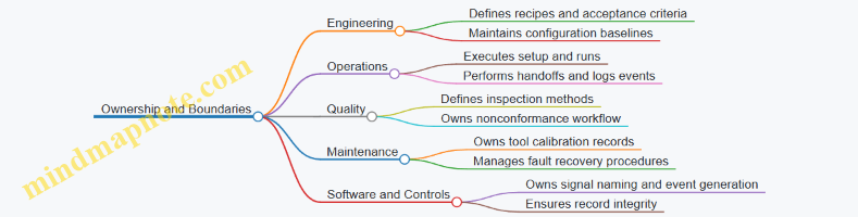
1.4 Establishing Common Terminology for Operations and Production Systems
Orbital manufacturing is a team sport: engineers, operators, software, quality, and maintenance all need the same words to mean the same things. Terminology is not paperwork for its own sake; it is how you prevent a “small misunderstanding” from becoming a bad part, a stuck tool, or a confusing incident report.
Start with three foundational layers. First, define objects: parts, tools, fixtures, consumables, and data artifacts. Second, define processes: the steps that transform objects, such as printing, machining, cleaning, joining, and inspection. Third, define operations: how processes are executed in time, including setup, run, handoff, and verification. When these layers are separated, you can reuse terms without mixing meanings.
A practical rule: every term should have (1) a plain-language definition, (2) a measurable scope, and (3) an ownership boundary. For example, “workcell” should not mean “the whole facility” in one document and “the robot station” in another. If you cannot point to the physical boundaries and the responsible team, the term is not ready.
Core Vocabulary for Objects, Processes, and Operations
Objects include:
- Part: the manufactured item that will be delivered or installed.
- Tool: an instrument that performs work, such as a print head, drill, or welding torch.
- Fixture: a device that holds or positions an object to control geometry.
- Consumable: material consumed or altered during a process, such as powder, wire, or abrasive media.
- Batch: a group of items processed under shared material and parameter conditions.
Processes include:
- Process Step: an atomic transformation, like “apply coating” or “measure diameter.”
- Recipe: the parameter set and logic that drives a process step.
- Inspection Method: the measurement or test technique used to verify requirements.
Operations include:
- Run: one execution of a recipe for a specific part or batch.
- Setup: pre-run actions that configure the workcell, tools, and environment.
- Handoff: the transfer point where responsibility and data move to the next step.
- Nonconformance: a deviation from defined requirements that triggers a defined response.
Standardizing Names for Interfaces and Data
Orbital systems rely on interfaces: mechanical, electrical, software, and procedural. Terminology should reflect that.
- Interface: a defined boundary between systems, described by inputs, outputs, constraints, and acceptance criteria.
- Signal: a named data channel or control line with a defined unit and meaning.
- Event: a timestamped occurrence used for traceability, such as “tool change complete.”
- Record: stored evidence tied to an event, run, or inspection.
A common failure mode is using the same word for both a physical action and a software state. For instance, “armed” should mean the physical readiness state, while “controller armed” can be the software state. If you keep these distinct, troubleshooting becomes faster.
Terminology for Quality and Traceability
Quality terms must be unambiguous because they drive decisions.
- Requirement: a stated condition the part must meet.
- Acceptance Criterion: the specific rule used to judge compliance.
- Concession: an approved deviation that still allows controlled use.
- Rework: a corrective process that returns an item to compliance.
- Scrap: disposition when compliance cannot be achieved within defined rules.
Traceability terms should also be consistent:
- Lot Control: how material batches are tracked.
- Process Trace: the parameter and event history for a run.
- Configuration: the exact set of software, hardware, and recipe versions used.
Example: A Single Production Thread with Consistent Terms
Consider a printed bracket.
- The operator performs setup for the print workcell.
- The system executes a run using a specific recipe.
- After printing, the bracket is moved to a handoff point for post-processing.
- The inspection method measures critical dimensions, producing a record tied to the run.
- If a dimension fails the acceptance criterion, the item becomes a nonconformance and is either reworked or scrapped based on defined rules.
Notice how each sentence uses a term that maps to a concrete action or artifact. That is the goal: words that behave like handles.
Mind Map: Common Terminology Map
Example: Term Definitions That Prevent Miscommunication
Use short definitions with measurable scope.
- Run: one execution of a recipe for one part or one batch, producing a process trace and inspection-ready state.
- Batch: items sharing the same material lot and recipe version, processed within the same controlled window.
- Event: a named, timestamped system occurrence that can be referenced in records.
When teams adopt these definitions, incident reports become consistent. A “missing record” is no longer a vague complaint; it is a specific absence of an expected record type for a named event within a run.
Mind Map: Ownership and Boundaries
The final step is governance: a single controlled glossary, versioned like any other configuration item. If the glossary changes, the change should be traceable to the documents and procedures that used the old terms. That way, the system can explain itself even when people rotate off shift.
1.5 Documenting Requirements Using Process Maps and Facility Interfaces
Orbital manufacturing is unforgiving about ambiguity: a missing requirement can become a tool collision, a scrap batch, or a quality escape. The goal of this section is to show how to document requirements so that (1) engineers agree on what must happen, (2) operators can execute it, and (3) interfaces between systems are testable.
Foundations for Requirement Clarity
Start with a simple rule: every requirement should be traceable to a process step and to an interface. If a requirement only says what you want, without where it is produced and who consumes it, it will be hard to verify.
A practical workflow begins with three artifacts:
- Process map: a step-by-step view of how work moves through the facility.
- Facility interface catalog: a list of system-to-system interactions (data, power, fluids, mechanical interfaces, safety signals).
- Requirement statements: short, verifiable sentences tied to a specific process step and interface.
To keep teams aligned, define a consistent naming scheme for process steps and interface endpoints. For example, label steps as P-03 and interface endpoints as IF-POWER-1, then reference them in requirement text.
Process Maps That Engineers Can Use
A process map should include more than arrows. Include the “inputs and outputs” at each step, the “decision points,” and the “handoffs” between workcells.
Use these elements:
- Step: a unit of work with a clear start and end condition.
- Input: material, part state, or data needed to begin.
- Output: the resulting part state or data produced.
- Controls: the parameters that must be set or monitored.
- Verification: how the step is accepted (measurement, inspection, or system status).
Example: In an orbital additive workflow, a step might specify that the part is printed in a defined orientation, then the output includes a “print completion record” with layer count and build time. That record becomes an input to inspection.
Facility Interfaces That Prevent Surprises
Interfaces are where requirements become real. Document them with enough detail to support integration testing.
For each interface, capture:
- Type: power, data, mechanical, thermal, vacuum, consumables, or safety.
- Direction: who provides and who consumes.
- Signals or parameters: what is exchanged (e.g., setpoints, status flags, alarms).
- Timing: when messages are valid and expected.
- Constraints: limits such as voltage ranges, allowable pressure, or maximum communication latency.
- Failure behavior: what happens when the interface is degraded.
A small but effective habit is to document interface failure behavior as a requirement. For instance, “If metrology camera status is unavailable for more than 10 seconds, the workcell must pause the inspection step and raise a specific alarm code.” That turns a vague risk into a testable outcome.
Mind Map: Requirement Documentation
Example: Turning a Process Step into Requirements
Consider a metrology step after machining.
-
Process map step:
P-07 Inspect machined feature.- Input: part in fixture
FX-2, datum reference established. - Output: measurement record
MR-07with feature diameter and surface roughness. - Verification: compare to acceptance limits.
- Input: part in fixture
-
Facility interface involvement:
- Data interface
IF-DATA-MET-1between metrology system and manufacturing execution software. - Mechanical interface
IF-MECH-FIX-2between fixture and part handling robot.
- Data interface
-
Requirement statements (each tied to
P-07and an interface):- “The metrology system shall transmit
MR-07to execution software viaIF-DATA-MET-1within 2 seconds of inspection completion.” - “The robot shall confirm fixture engagement status
FX-2-ENGAGEDbefore starting inspection, usingIF-MECH-FIX-2status signals.” - “If
MR-07is missing or incomplete, the execution software shall mark the part as nonconforming and prevent downstream coating steps.”
- “The metrology system shall transmit
Notice how each requirement states an observable behavior, not just an intention.
Advanced Details Without Losing the Plot
As complexity grows, keep documentation systematic:
- Use requirement templates so every statement includes: condition, action, interface, and measurable outcome.
- Separate process intent from interface mechanics. The process map explains what “inspection” means; the interface catalog explains how data and status travel.
- Record assumptions explicitly inside the process map notes, not inside requirement text. For example, “Assumes fixture
FX-2provides datum repeatability of X” belongs as a process map note tied to the fixture interface.
When done well, process maps and facility interfaces form a two-sided contract: one side describes the work, the other describes the connections. Requirements then become the bridge that lets teams test the system without guessing.
2. Orbital Environments and Their Impact on Production
2.1 Microgravity Effects on Material Handling and Process Stability
Microgravity changes how forces show up in everyday manufacturing steps. On Earth, gravity quietly does a lot of work: powders settle, liquids drain, chips fall away, and parts stay put in fixtures. In orbit, those same steps become force-management problems. The result is not “everything floats,” but “the dominant forces are different,” so process stability must be engineered rather than assumed.
Foundational Concepts for Handling in Orbit
Weightlessness is not forcelessness. Even in microgravity, objects still experience contact forces, surface tension, inertia, and momentum transfer. A robot pushing a part still has to overcome friction and adhesion, and a powder stream still needs a controlled path.
Momentum persists. When a tool or part moves, it carries momentum. If you stop suddenly, the reaction goes somewhere—often into the workpiece, the fixture, or the surrounding equipment. This is why “gentle” motion profiles matter for both safety and dimensional control.
Surface effects become louder. Without gravity-driven drainage, wetting and capillary behavior can dominate. Likewise, powder cohesion and electrostatic attraction can cause clumping or sticking to surfaces.
Material Handling Failure Modes and What Causes Them
-
Powder behavior shifts from settling to clumping. On Earth, gravity helps powders flow into hoppers and clears loose material. In microgravity, powder can bridge across openings or form stable agglomerates. A practical symptom is inconsistent feed rate during additive or inconsistent mass transfer during dosing.
-
Liquids do not drain reliably. Without gravity, a droplet may cling to a nozzle, spread across a surface, or remain trapped in corners. This affects coating uniformity, adhesive dispensing, and cleaning steps.
-
Chips and debris do not “fall away.” In machining, chips can remain near the cutting zone, increasing tool wear and contaminating subsequent steps. Even if the chips are moving, they may not clear the way you expect.
-
Workpiece positioning becomes more sensitive. Fixtures that rely on weight to maintain contact can lose effectiveness. A part can lift slightly, rotate under tool forces, or shift during thermal cycles.
Process Stability: Turning Physics into Controls
Process stability means the same inputs produce the same outputs within defined limits. In microgravity, stability depends on controlling contact, flow, and energy transfer.
Control contact forces. Use positive mechanical constraints when possible: kinematic mounts, vacuum clamping, or compliant fixtures that maintain normal force despite small disturbances. For example, a vacuum chuck can hold a machined coupon while a robot inserts it, preventing micro-motions that would ruin surface finish.
Control motion profiles. Limit acceleration and deceleration of moving tools and parts. If a robot arm must place a part into a tight tolerance interface, a short, smooth approach reduces reaction forces that could disturb the mating surfaces.
Control flow paths. For powders and liquids, design channels and reservoirs so material movement is driven by pressure, controlled gas flow, or capillary management rather than gravity. A simple example is using a funnel-like feed geometry with a controlled purge gas to prevent bridging.
Control thermal gradients. Microgravity does not remove heat transfer; it changes it. Convection is weaker, so conduction through fixtures and radiation become more important. If a heat treatment step assumes Earth-like cooling, dimensional drift can appear. Stabilize by using thermal contact paths and measuring temperature at the same interface that matters for the part.
Practical Examples That Make the Differences Concrete
Example: Powder Transfer for Additive Feed A powder dosing system that works on Earth by “letting powder settle” will underfeed in orbit. Replace settling with a controlled metering approach: meter by volume or mass using a sealed container, then deliver through a short, straight path with a gentle purge. Verify stability by tracking delivered mass over repeated cycles and checking for clumps on the outlet filter.
Example: Adhesive Dispensing Without Drip On Earth, gravity helps a nozzle stop dripping. In microgravity, the adhesive can form a filament that stretches and then snaps, leaving inconsistent bead geometry. Use a dispenser with a controlled cut-off valve and a brief dwell to let the bead relax under surface tension. Inspect bead width and cure uniformity at the same location each time.
Example: Machining Chip Management A machining setup that relies on chip fall will accumulate debris near the tool. Add a containment shroud and actively remove chips using a directed suction or controlled airflow inside the enclosure. Then confirm that the chip removal does not introduce vibration that would affect tool chatter and surface roughness.
Mind Map: Microgravity Handling and Stability
Summary of What to Engineer First
Start by identifying which material state is involved—powder, liquid, solid debris, or a workpiece interface. Then decide what force normally “solves” the step on Earth and replace that assumption with a deliberate mechanism in orbit: clamping that maintains contact, motion that limits reaction, flow paths that do not depend on settling, and thermal contact that does not rely on convection.
2.2 Radiation, Thermal Cycling, and Their Influence on Equipment and Materials
Radiation and Thermal Cycling in Orbital Manufacturing
Radiation and thermal cycling are two separate stressors that often show up together in orbital factories. Radiation changes materials and electronics by altering their internal structure, while thermal cycling repeatedly expands and contracts components as temperatures swing. In practice, the manufacturing impact is usually indirect: equipment drifts, sensors lie, coatings degrade, and tolerances slowly wander.
Radiation Basics for Equipment and Materials
Radiation in space is mainly high-energy particles and photons. When they pass through matter, they can create point defects, break chemical bonds, and generate charge in insulating layers. The result is not always immediate failure; it can be gradual property drift.
Key pathways include:
- Total ionizing dose: charge accumulates in dielectrics, shifting electrical thresholds in electronics and changing insulation behavior.
- Displacement damage: energetic particles knock atoms out of place, increasing brittleness and reducing performance in semiconductors and some structural materials.
- Surface charging and arcing risk: insulating surfaces can accumulate charge, especially near conductive structures, leading to localized discharges that can damage sensitive components.
A practical manufacturing example: a laser power supply uses control electronics with insulating layers. Over time, threshold shifts can cause the same command to produce slightly different output power. If the process assumes constant energy density, printed layers can become subtly under-melted or over-melted, even though the operator sees “normal” readings.
Thermal Cycling Basics and Why It Matters
Thermal cycling is the repeated change in temperature caused by orbital day/night cycles, station attitude changes, and heat rejection limits. Materials expand and contract according to their coefficients of thermal expansion, but assemblies rarely share the same expansion behavior.
That mismatch drives:
- Thermal strain in structures and tool mounts.
- Stress at interfaces such as brazed joints, adhesive layers, and thin coatings.
- Fatigue in fasteners and flexures due to cyclic loading.
- Dimensional drift in metrology fixtures and reference surfaces.
A concrete example: a precision machining workholding plate is mounted to a base with different thermal expansion. During a cycle, the plate’s flatness can change by microns. If the metrology routine measures after thermal stabilization but machining starts earlier, the part can be cut to the wrong geometry.
How Radiation and Thermal Cycling Interact
Radiation can change how materials conduct heat and how they respond to temperature. It can also affect lubricants, polymers, and adhesives by altering their chemistry. Thermal cycling then amplifies the consequences by repeatedly stressing the already-changed material.
Consider a robotic end effector with a polymer cable jacket and a grease-lubricated joint. Radiation can embrittle the polymer and harden the grease, while thermal cycling changes clearances and loads. The combined effect is more than additive: the joint may become noisier, then stickier, and finally unreliable at the exact moment you need repeatability.
Mind Map: Radiation and Thermal Cycling Effects
Systematic Mitigation Practices with Examples
1. Separate what you can measure from what you must model. For radiation, track dose proxies and component-level sensitivities. For thermal cycling, measure temperature at the actual interfaces that matter: tool tip, sensor mounting surface, and reference planes. Example: during commissioning, log temperature and metrology readings together so you can quantify how much a gauge block’s apparent size changes across a cycle.
2. Design for differential expansion. Use compliant mounts where appropriate, and choose materials with compatible expansion behavior for critical interfaces. Example: a coating deposition mask can be mounted with a flexure that maintains alignment even when the substrate expands.
3. Control thermal stabilization before precision steps. Many processes assume steady conditions. Example: pause between heating and first measurement in a coating cure workflow until the substrate reaches a stable temperature band, then start inspection.
4. Harden electronics and protect sensitive interfaces. Use radiation-tolerant components where required and route signals to minimize exposure. Example: place the most sensitive analog front-end closer to the controlled thermal zone and shield it from direct radiation paths.
5. Validate with representative cycling profiles. Equipment should be tested under temperature swings that mimic operational duty, not just a single soak temperature. Example: run a workcell through repeated thermal cycles while performing a repeatability check on a robotic pick-and-place datum.
Example Workflow: From Stressors to Quality Control
A practical chain looks like this: radiation causes gradual electronics drift, thermal cycling causes mechanical alignment drift, and both show up as process variation. The response is to add checkpoints that detect the drift early. Example: in an additive workflow, periodically print a calibration coupon, measure key dimensions, and correlate deviations with recent temperature history and equipment operating hours. When the coupon trend shifts, you adjust process parameters or schedule maintenance before the deviation reaches the tolerance limit.
2.3 Vacuum and Outgassing Considerations for Manufacturing Quality
Vacuum changes how materials behave, and those changes show up directly in manufacturing quality. In orbit, the chamber is effectively a high vacuum, so volatile molecules can escape from surfaces and contaminate nearby optics, sensors, and even the part you are trying to finish. The key quality idea is simple: if you can predict what leaves a material, you can control what deposits where.
Foundational Concepts for Vacuum Quality
Outgassing is the release of gas from a material due to dissolved gases, absorbed moisture, and low-molecular-weight components migrating to the surface. In vacuum, there is no ambient air to dilute those molecules, so local partial pressures rise near the source and transport by molecular flow.
Two practical distinctions matter for quality:
- Volatile content: how much gas can be released.
- Release rate: how quickly it comes out under the process temperature.
A common manufacturing mistake is treating “vacuum” as a single condition. In reality, quality depends on the vacuum level during each step: pump-down, dwell, processing, and cooldown. A part that looks fine at the end of a process may have been contaminated earlier when the chamber was still cleaning itself.
Outgassing Pathways and Where They Matter
Outgassing sources include polymeric binders, lubricants, adhesives, surface residues, and even some metals that trap gases in micro-voids. Moisture is a frequent culprit because it can desorb during heating and then react with other surfaces.
Quality impacts show up in three main ways:
- Deposition on critical surfaces: thin films can alter optical reflectivity, sensor response, or coating performance.
- Process instability: contamination can change laser absorption, plasma behavior, or thermal contact.
- Dimensional and surface changes: absorbed gases can expand and then leave, affecting surface finish and microstructure.
Mind Map: Vacuum and Outgassing Quality Chain
Control Methods That Actually Work
Material selection reduces the problem at the source. For example, if you need a temporary fixture inside the chamber, choosing a low-outgassing polymer instead of an unknown elastomer can prevent a visible haze on a nearby witness plate after a thermal step.
Cleaning and drying remove residues that desorb later. A practical workflow is: solvent clean, rinse with a compatible low-residue method, then dry under controlled conditions before assembly. In orbit-like vacuum, a “mostly dry” part can still release enough moisture to fog a nearby surface.
Bake-out and preconditioning are about matching the material’s release curve to your process. If a coating step occurs at 120°C, preconditioning at a similar or slightly higher temperature for a controlled duration can reduce the early burst of outgassing during the actual run. The quality win is that the chamber starts the real process with fewer contaminants already in flight.
Chamber conditioning and shielding manage where molecules go. Even with good materials, geometry matters. A simple approach is to position parts so that critical surfaces are not in direct line-of-sight with known outgassing sources like tooling, reservoirs, or cartridge housings.
Monitoring with pressure and witness samples turns assumptions into evidence. Pressure transients during pump-down can indicate a strong outgassing source. Witness coupons placed near sensitive areas can reveal deposition patterns without risking the actual part.
Example: Preventing Coating Contamination
Suppose you are applying a thin thermal-control coating to a small panel. The panel is mounted near a polymer cable guide used to route power and signals.
- During the first pump-down, the chamber pressure stabilizes slowly, suggesting a persistent gas source.
- After coating, the panel shows reduced reflectivity in a narrow region consistent with a deposition plume.
- The fix is twofold: replace the cable guide with a low-outgassing material and precondition it with a bake-out before installation.
- Add a witness plate at the same relative position as the panel’s sensitive area. After changes, the witness plate shows minimal film, and the panel’s reflectivity becomes uniform.
This example highlights a quality principle: you don’t just want “low outgassing,” you want low outgassing at the time the sensitive step is happening.
Advanced Details for Process Control
Temperature history is often the hidden variable. A part that is assembled at room temperature, then heated rapidly, can produce a short high-rate outgassing burst that deposits before the chamber reaches its steady state. Slower ramping or staged preconditioning can reduce that burst.
Another subtlety is re-exposure. If a part is removed from vacuum or exposed to humid handling between cleaning and processing, it can regain absorbed moisture. Quality control therefore includes handling discipline: minimize time in uncontrolled environments and keep assembly steps consistent.
Finally, treat tooling as a first-class quality item. Fixtures, clamps, and liners can outgas and contaminate the part even if the part material itself is well characterized. A “clean part” paired with “dirty tooling” is still a contaminated process.
Summary of Quality Levers
Quality in vacuum manufacturing comes from controlling the source, the timing, and the path of molecules. Choose low-outgassing materials, clean and dry thoroughly, precondition with bake-out aligned to your process temperature, manage geometry with shielding, and verify outcomes using pressure behavior and witness samples.
2.4 Orbital Dynamics That Affect Logistics and Station Keeping
Logistics in orbit is not just “moving stuff from A to B.” It is the choreography of timing, geometry, and forces. Station keeping is the ongoing work that keeps a platform where it needs to be so that docking windows, line-of-sight operations, and safe tool access remain predictable.
Foundational Geometry and Timing
Every logistics plan starts with where the platform is relative to the visiting vehicle and to the Sun. Orbital position is described by elements such as inclination and right ascension of the ascending node, but operations care about practical geometry: relative velocity at rendezvous, approach direction, and how long the platform remains in a favorable attitude for communications and payload handling.
A simple example: if a cargo vehicle must approach along a specific axis to avoid thruster plume contamination, then the platform’s attitude constraints effectively reduce the usable time window. Even when the orbit is correct, the “right time” might not overlap with the “right orientation.”
Relative Motion and Rendezvous Constraints
Rendezvous is governed by relative motion, not just absolute orbit. Two spacecraft can share a similar altitude yet still have a large along-track separation, meaning one is “ahead” or “behind” the other. Closing that gap requires carefully planned burns that change the relative trajectory.
Operationally, this affects logistics in three ways:
- Propellant budgeting: More along-track separation means more delta-v and more thruster time.
- Docking timeline: The approach corridor narrows as time passes, so late changes can force a different phasing strategy.
- Operational coupling: If station keeping is actively correcting drift, the vehicle may need to wait for a stable relative state before final approach.
A concrete example: a resupply mission scheduled for a tight docking window may still succeed if station keeping is “quiet” during the final hours. If the platform performs a corrective maneuver during that period, the relative motion profile shifts and the visiting vehicle may need additional guidance updates or a hold.
Perturbations That Drive Station Keeping
Orbits are rarely perfect circles. The main perturbations that matter for logistics are those that change the platform’s position and attitude over time.
- Atmospheric drag: Even at high altitudes, residual atmosphere slows the spacecraft slightly, shrinking the orbit and shifting the ground track. Drag is strongest near solar activity peaks and when the spacecraft’s effective area increases due to attitude.
- Gravity field irregularities: The Earth’s non-uniform gravity causes precession and changes in orbital elements, especially for long-duration missions.
- Third-body effects: The Moon and Sun tug on the orbit, producing slow but measurable changes in geometry.
- Solar radiation pressure: Light pressure can nudge the orbit and, more importantly, can influence attitude control loads.
A practical example: if a platform uses a large deployable radiator for thermal control, its effective area for drag and radiation pressure changes. That means station keeping maneuvers must account for the configuration, not just the baseline orbit.
Attitude, Thruster Plumes, and Operational Safety
Station keeping is often split into orbit control and attitude control, but logistics cares about their coupling. Thruster firings can create contamination risks, thermal shocks, and sensor blinding.
Consider a platform that must keep a docking port clean for a sensitive seal. If station keeping uses thrusters that point near the docking axis, then each maneuver becomes a logistics event: it may require a “settle time” before docking, inspection, or robotic handling.
A concrete workflow example:
- Plan a station keeping burn to occur after the cargo vehicle departs.
- Include a post-burn stabilization period for attitude sensors and thermal gradients.
- Verify that plume impingement constraints are satisfied for the next docking or for any operations that require direct line-of-sight.
Control Loops and Maneuver Planning
Station keeping is executed through control loops that estimate the current state, compute corrections, and command actuators. The key is that estimation errors and maneuver execution errors both affect logistics.
- State estimation: Navigation filters produce uncertainty ellipses. Larger uncertainty means larger safety margins in rendezvous planning.
- Maneuver execution: Thruster performance varies with temperature, propellant conditions, and valve timing. Small errors accumulate into along-track and cross-track offsets.
A simple example: if the platform’s orbit determination is updated less frequently, the computed phasing for a visiting vehicle may rely on older data. The result is a larger correction budget for the visiting vehicle, which can reduce its payload margin.
Mind Map: Dynamics to Logistics Link
Example: Putting It Together for a Docking Day
A platform schedules a cargo docking. First, it checks whether the planned station keeping burns keep the docking port within its attitude limits during the final approach. Next, it estimates how drag and radiation pressure will shift the orbit between the last navigation update and the docking time. Then it ensures the final maneuver does not violate plume constraints and includes a stabilization interval so sensors and thermal conditions settle.
If any piece fails—say, drag is higher than expected due to a configuration change—the platform can adjust by changing the burn timing or magnitude. The logistics impact is immediate: the visiting vehicle may need a different phasing plan, or the docking may move to a later window where the geometry and operational constraints align.
The takeaway is straightforward: station keeping is not background maintenance. It is the mechanism that makes logistics repeatable, because it controls the geometry, timing, and safety conditions that docking and handling depend on.
2.5 Environmental Monitoring and Data Logging for Process Control
Orbital manufacturing lives inside a moving set of conditions: microgravity changes how fluids behave, radiation nudges electronics, and thermal cycling can shift tolerances. Environmental monitoring turns those conditions into measurable inputs, so process control can respond with evidence instead of guesswork.
Foundational Concepts for Environmental Data
Start by separating three things: environmental variables, process variables, and quality outcomes. Environmental variables include vacuum level, chamber pressure stability, temperature fields, radiation dose rate, and vibration. Process variables include laser power, deposition rate, spindle speed, or cure temperature. Quality outcomes include dimensional error, surface roughness, porosity, bond strength, and coating adhesion.
A practical rule: log environmental variables at a rate high enough to capture changes that could affect the process, but not so high that storage becomes a bottleneck. For example, if a thermal control loop cycles every 30 seconds, logging temperature once per second is usually sufficient to see the cycle shape and correlate it with process drift.
Sensor Selection and Placement Logic
Sensors must measure what matters and do so consistently. Placement is not cosmetic; it defines what the data means.
- Temperature: Place sensors near thermal gradients that influence the workpiece, not only on the chamber wall. If a part sits on a fixture, measure fixture temperature and chamber air or gas temperature separately.
- Pressure and Vacuum: Use a pressure gauge appropriate to the operating range. A high-quality vacuum reading is useless if it is delayed by plumbing volume; choose locations that reflect the chamber where the process occurs.
- Radiation and Total Ionizing Dose: For electronics protection and data integrity, monitor dose rate at or near sensitive electronics. For process effects, radiation-sensitive materials may require additional monitoring at the work volume.
- Vibration and Shock: Mount accelerometers on the structure that carries the tool or workholding. If you measure only the platform frame, you may miss tool-specific vibration.
A simple sanity check: if moving a sensor changes the reading but not the process outcome, you likely measured the wrong location or the wrong variable.
Data Logging Architecture for Traceable Control
Environmental data logging should support three tasks: real-time control, offline verification, and traceability.
- Real-time control: Provide fast signals to controllers. Example: if chamber temperature rises beyond a setpoint during additive manufacturing, the controller can pause deposition and adjust thermal power.
- Offline verification: Store higher-resolution logs for later correlation. Example: if a batch shows increased voids, you can compare void statistics against pressure stability and temperature gradients.
- Traceability: Link each log segment to a specific job, material lot, tool configuration, and recipe revision.
Use synchronized timestamps across all data streams. In microgravity operations, a 5–10 second mismatch between process and environment logs can scramble cause-and-effect analysis.
Data Quality Rules That Prevent Bad Decisions
Environmental monitoring fails when the data is wrong, incomplete, or misleading. Apply explicit rules:
- Calibration status: Record calibration date, calibration method, and last verification result for each sensor.
- Range checks: Flag readings outside physical plausibility. Example: a vacuum gauge reporting 10^-2 Pa during a process that requires 10^-5 Pa should trigger an alarm and mark the dataset as suspect.
- Staleness checks: If a sensor stops updating, treat it as missing data rather than holding the last value.
- Noise characterization: Track sensor noise level so you can distinguish real process-linked changes from measurement jitter.
Mind Map: Environmental Monitoring to Process Control
Example: Correlating Thermal Drift with Dimensional Error
Suppose an orbital machining cell produces a set of brackets with a consistent hole diameter bias. Environmental logs show fixture temperature rising by 6°C over the first 3 minutes of each job, then stabilizing. Process logs show spindle speed and feed rate remain within tolerance.
The control action is straightforward: add a preheat soak step and require fixture temperature to reach a target band before starting the cutting cycle. The evidence trail is equally important: the log now proves that each job began only after the thermal condition was met, and the dimensional bias disappears.
Example: Vacuum Stability During Coating
A thin-film coating run depends on stable pressure to control deposition conditions. During one batch, pressure logs show intermittent spikes aligned with a valve cycling pattern. The coating thickness map later reveals streaks in the same time windows.
Instead of blaming the coating recipe, the monitoring data points to the vacuum system behavior. The fix is to adjust valve timing and add a rule: if pressure exceeds a spike threshold for more than a defined duration, the system pauses and resumes only after pressure returns to the stable band.
Operational Practices for Logging Without Overhead
To keep logging useful rather than burdensome:
- Log raw sensor streams for investigation and derived features for control, such as moving averages of pressure and temperature gradients.
- Store event markers like recipe start, tool change, and chamber pump-down completion so analysts can navigate long runs quickly.
- Use a consistent naming scheme for jobs and sensors, and include the sensor’s calibration verification date. For example, a verification performed on 2026-03-01 should be recorded so later audits can interpret sensor behavior correctly.
Environmental monitoring is not a separate activity from process control; it is the measurement layer that makes control decisions defensible. When sensors are placed correctly, data is synchronized, and quality rules are enforced, the logs become a reliable map from conditions to outcomes.
3. Facility Architectures for Space Based Production
3.1 Platform Topologies for Manufacturing Modules and Service Modules
A manufacturing platform in orbit is rarely “one big factory.” It’s a set of modules arranged so that tools, materials, power, thermal control, and data can move through the system with predictable interfaces. A topology is the blueprint for how those modules connect and how work flows between them.
Foundational Concepts for Topology Choices
Start with three questions. First, what must be co-located for process physics? For example, additive printing needs a stable thermal and vibration environment around the build volume, so the printer module is typically paired tightly with its local power conditioning and thermal interface. Second, what can be separated by logistics? A metrology station can be physically distinct if parts can be transferred without losing alignment or cleanliness. Third, what must be shared? Service modules often provide common capabilities like cryogenic or high-pressure gas handling, waste management, or spare tool storage.
A useful rule: separate modules when the interface is measurable and controllable. If two modules share a “soft” interface like informal handling practices, keep them closer.
Core Topology Patterns
1) Linear Production Line Modules are arranged in a sequence: material prep → forming/printing → joining/coating → inspection → staging. This reduces routing complexity because parts travel forward with minimal backtracking. In microgravity, the “forward motion” is often handled by robotic transfer and fixtures rather than gravity, but the logic stays the same.
Example: A small platform prints a bracket, transfers it to a curing station, then to a coordinate measurement station. Each transfer uses the same docking interface on the part carrier, so the inspection program can assume a consistent datum.
2) Hub and Spoke with a Central Service Hub A central service hub connects to multiple manufacturing spokes. Spokes include workcells for specific processes, while the hub provides shared utilities and logistics routing.
Example: Three workcells—machining, welding, and surface coating—share a common waste and consumables handling module. The hub also hosts a standardized tool-change bay, so each workcell can request a tool cartridge without redesigning its own storage.
3) Cell Clusters with Local Utilities Each cluster contains a manufacturing module plus its immediate utilities and inspection. Clusters are then connected by a logistics corridor.
Example: A cluster dedicated to additive manufacturing includes the printer, powder handling, and in-process monitoring. Another cluster handles machining and metrology. This topology limits cross-contamination risk because powder and debris stay within the additive cluster.
Interface Engineering for Modules
Topology succeeds or fails at interfaces. Treat interfaces as contracts with three layers: mechanical docking, utilities, and software.
- Mechanical docking: Use repeatable alignment features so a part carrier or tool cartridge returns to the same coordinate frame. A practical approach is a kinematic mount with hard stops and a single reference pin.
- Utilities: Define power ranges, thermal rejection paths, and fluid or gas connections by standardized couplings. For instance, a coating module should specify allowable solvent flow rates and exhaust conditions so the service hub can route safely.
- Software: Manufacturing execution needs consistent identifiers for parts, fixtures, and tool cartridges. If a tool cartridge is swapped, the system should automatically load the correct process recipe and calibration offsets.
Service Modules and Their Placement Logic
Service modules exist to keep manufacturing modules focused on process work. Common service functions include:
- Logistics and staging: buffering parts between workcells.
- Tool storage and exchange: managing cartridges, nozzles, cutters, and calibration artifacts.
- Waste and debris management: capturing chips, powder, fumes, and contaminated wipes.
- Utilities distribution: power conditioning, thermal loops, and controlled atmospheres.
Placement depends on what must be kept clean. If a process generates fine particulates, keep its waste handling close to the source. If a service module is “clean by design,” place it so manufacturing debris cannot migrate through shared air paths or common handling rails.
Mind Map: Topology Building Blocks
Example: Choosing a Topology for a Multi-Process Subsystem
Suppose you need a subsystem that includes a printed housing, machined mounting faces, and a thermal-control coating.
A practical arrangement is a cell cluster for additive printing plus local powder handling, connected to a linear segment for machining and inspection, with a hub providing shared utilities and waste routing. The printed housing moves from the additive cluster to machining using the same carrier docking interface, so the machining program can reference the same datum. The coating step then uses a dedicated exhaust and cleaning boundary, but it can still draw power and thermal services from the hub.
This combination avoids two common failure modes: redesigning interfaces at every step, and letting debris-heavy processes share the same service pathways as cleanliness-sensitive ones.
3.2 Power, Thermal, and Data Distribution for Industrial Workflows
Industrial work in orbit is less about “having enough” and more about distributing three scarce resources—power, heat handling, and information—so every workcell gets what it needs at the right time. A practical distribution design starts with workload characterization, then turns that into electrical, thermal, and network requirements with explicit interfaces.
Foundational Inputs for Distribution Design
Begin by listing each manufacturing step as a workload block: tool power draw, duty cycle, peak current, required voltage rails, and start-up behavior. Add thermal outputs as heat-per-step and heat-per-minute, including transient spikes from lasers, heaters, and motorized axes. Finally, define data needs per step: control loop bandwidth, sensor sampling rates, file sizes for inspection images, and latency tolerance for safety interlocks.
A simple example: a powder-bed printer might have a modest average power draw but a sharp peak during laser firing, plus steady heat from electronics. A CNC step might have lower peak power but continuous motor load and frequent encoder reads.
Power Distribution Architecture
Use a layered approach: generation and conversion, distribution, local regulation, and protection. In practice, the platform typically provides one or more DC buses, then each workcell uses local DC-DC conversion for tool-specific rails. Protection is not optional paperwork; it is how you keep a single fault from turning the whole line into a short circuit.
Key best practices with concrete examples:
- Segment by function and duty cycle. If the printer and the metrology station share a bus, a printer peak can cause metrology brownouts. Put them on separate feeders or add buffering.
- Design for inrush and brownout. A vacuum pump or heater controller can draw a large inrush current. Add soft-start or staged enable so the bus voltage stays within limits.
- Use selective protection. Place fuses or solid-state breakers close to the load so upstream protection trips only the affected branch.
- Provide local energy buffering where timing matters. A small capacitor bank or supercapacitor module near a laser driver can smooth short peaks.
Thermal Distribution Architecture
Thermal distribution is the “plumbing” of heat removal. In microgravity, convection is limited, so heat must move through conduction paths to radiators or heat sinks. Treat thermal design as a network: each tool has a thermal resistance to a cold plate, and the cold plate has a resistance to the radiator.
Best practices with examples:
- Separate heat sources by temperature level. A high-temperature furnace and a sensor suite should not share the same cold plate without thermal isolation. Use intermediate heat exchangers or dedicated cold plates.
- Model transient heat loads. A laser step can create a short-lived thermal spike that causes drift in nearby metrology. Add thermal mass or schedule metrology after stabilization.
- Instrument the thermal path. Place temperature sensors at the tool interface and on the cold plate. If tool temperature rises while cold plate temperature stays flat, the issue is local conduction or contact quality.
- Control contact quality. A loose clamp or degraded thermal interface material can double thermal resistance. Build a repeatable mounting procedure and verify it during commissioning.
Data Distribution Architecture
Data distribution should match the control structure. Safety interlocks and motion control require deterministic behavior; inspection data and logs can tolerate more latency. A common pattern is to separate real-time control traffic from bulk data traffic.
Best practices with examples:
- Use a two-plane network. One plane for real-time control and safety signals, another for telemetry, inspection images, and maintenance logs.
- Define message classes and priorities. For example, emergency stop signals get the highest priority and minimal hops; camera frames for defect detection get lower priority and are buffered.
- Plan for bandwidth and storage. If a microscope produces large images every cycle, ensure the workcell controller can buffer locally and upload without blocking control loops.
- Make time synchronization explicit. Use a single time base so power events, thermal readings, and inspection results align. Otherwise, troubleshooting becomes guesswork.
Integrated Workflow Example
Consider a three-step workflow: print a bracket, machine its mounting face, then inspect it.
- Power: The printer feeder supplies peak laser power; the machining feeder supplies continuous motor load. The inspection station uses a stable rail and waits for machining to finish.
- Thermal: Printing generates heat that warms the cold plate; machining follows after a stabilization window so metrology doesn’t chase thermal drift.
- Data: Real-time motion commands run on the control plane, while inspection images transfer on the data plane. Time-stamped events link each step’s power and temperature history to the final measurement.
Mind Map: Power, Thermal, and Data Distribution
Practical Checklist for Commissioning
Before running production, verify each distribution interface with a controlled test: confirm power rails stay within tolerance during worst-case tool starts, confirm cold plate temperatures track expected heat loads, and confirm that control-plane messages meet timing while inspection-plane transfers do not interfere. If any of these fail, fix the interface first, not the symptom.
3.3 Cleanliness Control and Contamination Management Strategies
Cleanliness control in orbital manufacturing is less about “sterile vibes” and more about preventing specific failure modes: particle-induced shorts, coating defects from surface films, and process drift caused by outgassing or residue. In practice, you manage cleanliness as a system with inputs, controls, verification, and corrective actions.
Foundational Concepts for Orbital Cleanliness
Start by defining what “clean” means for each product and process step. A printed polymer bracket may tolerate more surface residue than a bonded thermal-control coating. Build a cleanliness requirement matrix that links:
- Item criticality (electrical, optical, sealing, structural)
- Process sensitivity (bonding surface prep, deposition, curing)
- Acceptable contamination types (particles, films, volatiles, moisture)
- Measurement method (visual inspection, swab analysis, mass change, particle counts)
Then separate contamination sources into three buckets:
- External: incoming parts, tools, packaging, and crew/robot handling.
- Internal: process byproducts like powder dust, chips, fumes, and cleaning solvents.
- Environment-driven: vacuum exposure, thermal cycling, and airflow patterns inside the module.
A simple rule keeps teams aligned: if a contamination source cannot be controlled at the source, it must be isolated by containment or removed by a defined cleaning step.
Cleanliness Zones and Workflow Discipline
Use cleanliness zones to prevent “clean work” from being interrupted by “dirty work.” Even without a full cleanroom, you can create functional zones with physical separation and procedural boundaries.
A practical zoning approach:
- Zone A: Receiving and staging for incoming materials and sealed containers.
- Zone B: Preparation for cleaning, surface prep, and tool setup.
- Zone C: Critical processing for bonding, deposition, curing, and metrology.
- Zone D: Waste and maintenance for chip/powder handling and tool servicing.
Workflow discipline means tools and consumables move one direction: A → B → C, with returns only through a defined decontamination path. For example, a robot end effector used to place a coated optical component should not later pick up loose powder unless it has been cleaned and verified.
Contamination Control Methods That Actually Work
Particle Control
Particles are the most visible problem and the easiest to underestimate. In microgravity, particles don’t “fall away,” so you need containment and capture.
- Use enclosed tool heads for powder handling and machining operations.
- Apply local vacuum extraction at the point of generation.
- Keep surfaces covered when not actively processing.
Example: During additive manufacturing, a powder transfer line should be purged and sealed between batches. If you open the line in Zone C, you’ve effectively moved the contamination source into the critical zone.
Film and Residue Control
Films from oils, fingerprints, polymer outgassing, and cleaning agents can ruin bonding and coatings.
- Specify compatible cleaning agents and rinse/evaporation steps for each material pair.
- Control wipe materials and their cleanliness level.
- Limit time between cleaning and critical processing so residue doesn’t re-form.
Example: If a surface prep step uses solvent wipes, schedule bonding immediately after drying and document the maximum allowable delay. A “later is fine” habit is how you end up with inconsistent bond strength.
Volatile and Outgassing Control
Vacuum and thermal cycling change how volatiles behave. Manage them by:
- Preconditioning materials and tools when required by the process.
- Using vented enclosures for steps that release fumes.
- Selecting adhesives, primers, and lubricants with known outgassing behavior.
Example: A curing step performed in an enclosure with poor exhaust can deposit volatiles onto nearby parts, creating haze or adhesion failures.
Verification and Measurement Strategy
Verification should be step-linked, not a single end-of-line surprise.
Common verification methods:
- Visual and microscopy for particles and surface defects.
- Swab or coupon sampling for residue and film presence.
- Mass change for certain cleaning effectiveness checks.
- Process parameter correlation where contamination affects outcomes (e.g., coating uniformity).
Use acceptance criteria tied to risk. For instance, a particle count threshold for electrical connectors should be stricter than for a non-critical bracket.
Corrective Actions and Nonconformance Handling
When contamination is detected, treat it like a root-cause problem, not a one-off cleanup.
A structured response:
- Quarantine affected items and any shared tools.
- Identify the contamination type (particles vs residue vs volatiles).
- Trace the workflow path to find where the source entered the critical zone.
- Update controls: change handling steps, improve containment, or adjust cleaning timing.
- Re-verify using the same method that found the issue.
Example: If swab results show solvent residue after bonding, the likely causes are incomplete drying, wrong wipe/agent, or excessive delay before bonding. Fixing only the last step wastes time and repeats the failure.
Mind Map: Cleanliness Control System
Example Workflow for a Bonded Assembly
A bonded thermal-control assembly illustrates the integrated approach. Incoming parts are staged in Zone A. Tools are cleaned and prepared in Zone B with documented wipe materials and drying time. The assembly is moved to Zone C where bonding occurs within the defined post-cleaning window. After curing, metrology is performed without opening the enclosure to Zone D. If residue is detected by swab sampling, the team quarantines the batch and the shared tools, then revises the drying and transfer timing rather than repeating only the final inspection.
3.4 Structural Design Interfaces for Tooling and Handling Systems
Structural design interfaces are the “handshake” between a manufacturing tool and the rest of the orbital platform. They must transmit forces and moments without unwanted motion, while also protecting the tool from contamination, thermal stress, and misalignment. In practice, the interface is more than a bolt pattern: it is a stack of mechanical, thermal, electrical, and procedural assumptions that must stay true from integration through production.
Interface Foundations and Load Paths
Start by defining the load path. A tooling interface should specify what loads it carries (axial force, shear, bending moment, torque), where they enter the structure, and what the structure must do in response. A simple example is a drilling head mounted to a robotic wrist: the drill thrust and cutting torque create axial and torsional loads that must be reacted by a stiff mount, not by compliant fasteners.
A practical way to avoid surprises is to separate “primary” and “secondary” constraints. Primary constraints prevent motion that would ruin process accuracy (for example, radial play at the tool axis). Secondary constraints help with alignment and retention (for example, locating pins that prevent rotational drift during handling). If you skip this separation, you often end up using the wrong element as the main load carrier, which leads to loosening or gradual misalignment.
Kinematic Location and Repeatability
Interfaces should establish repeatable positioning. Use a deterministic locating scheme: typically a combination of a rigid datum surface and one or more features that control the remaining degrees of freedom. For orbital tooling, repeatability matters because tools may be swapped for maintenance or because the platform experiences small attitude changes.
Example: a modular fixture plate for additive post-processing. If the plate is located only by bolts, the clamping force can vary with assembly torque and surface condition. Adding two hardened locating pins and a flat datum surface makes the location repeatable even when clamping force changes slightly.
Clamping, Fasteners, and Joint Integrity
Clamping is both mechanical and procedural. The interface should state required torque ranges, acceptable surface conditions, and whether preload is maintained through thermal cycles. In microgravity, you still get joint relaxation from temperature changes; the difference is that debris and loose parts are harder to manage.
A good rule is to design the joint so that the tool loads do not significantly alter preload. That means choosing fasteners and joint geometry that keep the interface in the elastic regime. Example: a machining tool adapter that uses a conical seat can reduce sensitivity to small misalignment because the seat self-centers, but it must be cleaned and inspected to prevent galling.
Thermal Expansion and Material Pairing
Orbital manufacturing tools see temperature gradients from heaters, lasers, and environmental cycling. Interface design must account for differential expansion between tool steel, aluminum structures, and any composite adapters.
Instead of treating thermal effects as an afterthought, incorporate them into the interface stack-up. Decide whether the interface should be thermally compliant (allowing controlled movement) or thermally stiff (maintaining alignment at the cost of higher stress). Example: a coating deposition head mounted near a thermal control panel. If the head must maintain a fixed standoff distance, use materials and geometry that minimize relative motion, and include a measurement plan to verify standoff after thermal stabilization.
Structural Stiffness, Damping, and Vibration Control
Even if the tool is accurate, the interface can ruin it by flexing under load or by amplifying vibration. Structural stiffness should be evaluated for the relevant load cases: cutting forces, handling impacts, and robot acceleration.
Damping is often overlooked. If the interface is a thin plate or a stack of dissimilar materials, it may ring. Example: a fixture for precision grinding. A stiff base with a constrained layer damping insert near the interface can reduce chatter without changing the grinding head design.
Contamination Management at the Interface
Interfaces must prevent contamination transfer between tooling and the work area. This includes particulates from machining, powder residue from additive processes, and outgassing from seals.
Design the interface with physical barriers and controlled flow paths. Use covers, wipers, or labyrinth features where appropriate, and ensure that any seals are compatible with the process environment. Example: a powder-handling nozzle adapter. A simple removable shroud around the adapter can catch stray powder during tool changes, keeping the mating surfaces clean enough for repeatable alignment.
Mechanical Protection During Handling and Tool Changes
Tooling interfaces experience impacts during docking, robotic pick-and-place, and maintenance operations. Add features that tolerate misalignment during engagement while still achieving precision once seated.
Example: a tool changer interface with chamfered lead-in surfaces. The chamfers guide the tool into position even if the robot has small positioning errors. Once seated, locating pins take over to control final alignment.
Mind Map: Structural Interface Design Checklist
Example: Interface Specification for a Robotic Machining Fixture
Define the interface in layers: (1) locating, (2) load transfer, (3) thermal behavior, (4) contamination control, and (5) verification.
A concrete specification might include: a flat datum surface for base seating; two hardened locating pins for lateral and rotational control; a bolt circle sized for cutting thrust and torque with preload that remains elastic across expected temperature swings; a removable shroud to prevent chips from reaching the mating surfaces; and a verification step that measures tool-to-work standoff and runout after thermal stabilization.
The result is not just a mechanical connection. It is a repeatable system boundary that makes the tooling behave the same way every time it is installed, even when the platform is doing what platforms do: moving, heating, and keeping the job on track.
3.5 Human and Robotic Workcell Integration for Production Operations
Human-robot integration in an orbital manufacturing workcell is mostly about making responsibilities unambiguous. A good starting point is to treat the workcell as a set of roles—operator, robot, inspection station, and material handler—then define what each role can do, what it must never do, and how it hands off work.
Foundational Concepts for Role Clarity
Begin with a task inventory. Break every production step into atomic actions such as “pick part,” “place in fixture,” “start process,” “verify measurement,” and “record traceability.” For each action, specify the success criteria in plain terms: correct location within tolerance, correct orientation, correct tool state, and correct data captured. Then assign an execution mode: robot, human, or shared.
A practical rule: if an action requires consistent force, repeatable motion, or controlled approach angles, prefer the robot. If an action requires judgment under uncertainty—like deciding whether a part is damaged beyond repair—keep a human in the loop. In microgravity, “judgment” often means checking containment integrity and confirming that the part is actually where the system thinks it is.
Workcell Interfaces and Physical Handshakes
Integration fails when the robot and the human “agree” only in software. Physical handshakes make the agreement real. Use fixtures that constrain the part in at least two degrees of freedom, and design end effectors to match those constraints. For example, a gripper that relies on friction alone is fragile; a fixture with a keyed pocket lets the robot place the part consistently even if the gripper grip varies slightly.
Containment is another interface. If you use a glovebox-like enclosure or localized containment around a process, define where the robot operates and where the human can safely intervene. A simple boundary can be enforced by interlocks: the robot must retract to a defined pose before the enclosure is opened, and the human must confirm the pose before resuming.
Safety Boundaries and Operational Modes
Define operational modes that map to real actions. Common modes include “automatic,” “manual teach,” “maintenance,” and “recovery.” Each mode should lock out specific behaviors. For instance, in maintenance mode the robot can move only within a reduced envelope, and it cannot start a process that would require stable thermal or vacuum conditions.
Recovery deserves explicit design. If a sensor indicates a mismatch—part not detected, tool not seated, or measurement out of range—specify the recovery sequence: stop motion, retract, request human confirmation, and log the event with enough context to reproduce the situation later.
Control Architecture for Predictable Handoffs
A robust integration pattern uses a manufacturing execution layer to coordinate steps while the robot controller handles motion. The execution layer should command “states,” not individual micro-movements. Example states: “fixture ready,” “part loaded,” “process enabled,” “inspection complete,” and “part released.” The robot then executes the motion required to reach the commanded state.
This state approach makes it easier to add a human checkpoint. Suppose the system completes “inspection complete” but the result is borderline. The execution layer can route to “human review required,” where the operator confirms the part using a defined measurement method and then either authorizes release or triggers a rework path.
Mind Map: Human and Robotic Integration Structure
Example: Pick, Inspect, and Release with a Human Checkpoint
Imagine an orbital workcell that assembles a small precision bracket. The robot picks the bracket from a contained magazine, places it into a keyed fixture, and runs a camera-based inspection. If the inspection score is above a threshold, the execution layer commands “release.” If the score is below threshold but not a hard fail, the system transitions to “human review required.”
The operator then performs a defined action: verify the bracket seating using a go/no-go gauge and confirm the fixture latch status. The system records the operator confirmation, then either authorizes release or routes to “rework required,” where the robot removes the part and reattempts placement after checking the fixture cleanliness.
Example: Maintenance Intervention Without Losing Traceability
During a routine tool change, the robot must retract and lock in a maintenance pose. The operator performs the swap, then confirms tool identity via a keyed connector and a simple readout. Only after the execution layer receives the confirmation does it allow the robot to return to automatic mode. Every step is logged: tool identity, operator confirmation, and the next production batch linkage.
Procedures That Make Integration Work in Practice
Integration is not only hardware and software; it is also procedure design. Use checklists for operator actions that the system cannot verify automatically, such as confirming a containment seal is intact or verifying a manual gauge reading. For robot actions, keep teach procedures consistent: record the reference frames used for calibration, and require a repeatable validation move before production resumes.
Finally, ensure every handoff produces data. When a human intervenes, capture the reason code and the method used. When the robot completes a step, capture the commanded state, the sensor evidence, and the part identifier. In a space manufacturing workflow, “who did what” is less about blame and more about making the next troubleshooting step fast and accurate.
4. Manufacturing Process Selection and Process Qualification
4.1 Criteria for Selecting Processes Compatible with Orbital Constraints
Choosing a manufacturing process for orbit is less about picking the “best” method and more about matching process behavior to the environment and the facility. A good selection starts with constraints you cannot negotiate—microgravity, vacuum, radiation, power/thermal limits, and contamination rules—then checks whether the process can still hit required tolerances, throughput, and safety.
Foundational Requirements
Begin with the product’s non-negotiables: geometry, material, allowable defects, and required performance. For example, a structural bracket may tolerate minor surface roughness but cannot tolerate dimensional drift that breaks fit-up. A thermal-control coating may tolerate small thickness variation but cannot tolerate contamination that ruins emissivity.
Next, define the production context. Is the process intended for a single item, a batch, or a recurring line? In orbit, setup time and consumables often dominate. If the process requires frequent calibration or consumable-heavy cleaning, it may be technically feasible but operationally expensive.
Finally, establish the interface to the facility: available power range, heat rejection method, allowable plume or particulate release, and the available metrology tools. If you cannot measure the result in the same facility, you are selecting blind.
Orbital Constraint Checklist
Use a structured checklist so decisions stay consistent.
- Microgravity behavior: Does the process rely on gravity for material flow, chip evacuation, or melt pool stability? If yes, you need containment, forced flow, or redesigned workholding.
- Vacuum and outgassing sensitivity: Will the process produce volatiles that contaminate optics, sensors, or adjacent hardware? If the process uses polymers, adhesives, or fluxes, you must verify outgassing limits.
- Radiation and thermal cycling: Will radiation degrade materials used in the process, or will thermal cycling change dimensions after curing or heat treatment?
- Power and thermal budget: Can the process run within the facility’s electrical limits and can it reject heat without overheating nearby subsystems?
- Contamination control: Does the process generate particulates, aerosols, fumes, or powder that must be captured? If containment is mandatory, confirm the process still performs inside the containment envelope.
- Safety and failure modes: Consider what happens on a misfire, power interruption, or tool jam. A process that fails “cleanly” is easier to recover than one that leaves reactive residue.
Process Capability Mapping
Once constraints are listed, map each candidate process to capability categories.
- Dimensional control: achievable tolerance, repeatability, and sensitivity to tool wear.
- Material compatibility: feedstock form (powder, wire, sheet, bulk), melting/processing temperature range, and joining compatibility.
- Surface and subsurface quality: roughness, porosity, microcracks, and residual stress.
- Inspection compatibility: whether the process leaves measurable signatures for in-facility inspection.
- Throughput and setup: time per part, changeover steps, and calibration frequency.
A practical rule: if a process’s quality depends on a parameter you cannot measure or control in orbit, it should be treated as “research-grade,” not “production-grade.”
Example: Additive vs. Subtractive Under Microgravity
Suppose you need a small lattice component.
- Additive manufacturing can be selected if you can manage powder or feedstock containment and if the melt pool behavior is stable under your thermal and motion conditions. You also need a plan for powder handling and post-build cleaning that does not spread contamination.
- Subtractive machining can be selected if you can hold the part rigidly and evacuate chips using vacuum or engineered chip channels. If chips float and contaminate optics, the process may still work, but only with robust capture and cleaning steps.
The decision is not “additive is easier” or “subtractive is cleaner.” It is whether each process’s failure modes and byproducts fit the facility’s containment and recovery procedures.
Mind Map: Selecting Processes for Orbital Compatibility
Decision Workflow That Avoids Surprises
- Start with product requirements and translate them into measurable acceptance criteria.
- Apply the orbital constraint checklist to each candidate process and record which constraints are handled by design versus by procedure.
- Map capability categories to your acceptance criteria, explicitly noting which parameters are controllable in orbit.
- Validate inspection compatibility by confirming you can measure the key quality attributes where the process runs.
- Review failure modes and recovery steps, ensuring the process can be restarted or safely shut down without contaminating the facility.
If you follow this sequence, the selection becomes a chain of evidence rather than a list of preferences. That’s the difference between a process that works in a lab and one that works on a platform.
4.2 Process Qualification Plans for Space Use Cases
A process qualification plan is the document that turns “it works on Earth” into “it works in orbit, with controlled risk.” For space manufacturing, qualification must prove not only that the process can produce conforming parts, but also that it can do so repeatedly under the constraints of microgravity, vacuum, radiation, limited access, and strict traceability.
Foundations of Qualification
Start by defining the process boundary: what steps are included, what interfaces are fixed (tooling, fixtures, software versions, gas lines, power profiles), and what variables are allowed to change. A good plan lists the process inputs and outputs in plain terms. For example, in an orbital additive step, inputs include feedstock lot, laser power setting, scan strategy, and chamber pressure; outputs include part geometry, surface roughness, and defect indicators.
Next, identify the qualification level. Some steps only need verification that they run safely and consistently (for example, a cleaning cycle). Others require full qualification because they directly affect critical performance (for example, a joining process that must survive thermal cycling). This distinction prevents over-testing everything and under-testing what matters.
Qualification Strategy and Evidence
A systematic plan uses a staged evidence ladder:
- Feasibility evidence shows the process can run in the relevant environment. Example: demonstrate that a powder handling method transfers material without excessive loss in a microgravity simulation setup.
- Capability evidence shows the process can meet requirements with statistical stability. Example: run multiple builds using controlled parameter sets and confirm dimensional capability.
- Robustness evidence shows the process tolerates realistic variation. Example: vary feedstock moisture within allowed limits and confirm the defect rate stays within acceptance.
- Integration evidence shows the process works inside the full workflow. Example: confirm that post-processing metrology and rework steps do not invalidate earlier steps.
Each stage should specify what data will be collected, how it will be analyzed, and what decision it supports.
Mind Map: Qualification Plan Structure
Test Article Selection and Worst-Case Thinking
Qualification is only as good as the test articles. Use representative geometry for functional steps and coupons for isolating variables. For instance, if a joining process is sensitive to surface prep, include specimens that intentionally span the expected roughness range. If a coating step is sensitive to substrate cleanliness, qualify with substrates that reflect the real cleaning process, not a “perfect” lab surface.
Worst-case selection should be explicit. A plan can define worst-case as the combination of parameter extremes that still occur in normal operations. Example: if the orbital power supply can vary by ±2% and the control system compensates, qualification should include runs at the compensated extremes, not only nominal settings.
Test Setup Control and Traceability
Qualification plans must treat setup as part of the process. Record calibration status for sensors used in control loops, document fixture alignment methods, and lock software versions for process execution. A practical example: if a machining step uses a tool offset table, qualification should verify that the offset update procedure is deterministic and that the table version is traceable to each part.
Traceability should be end-to-end. For each test run, capture material lot identifiers, consumable batch numbers, and the exact parameter set used. If a defect is found, the plan should make it possible to reconstruct the run without guessing.
Data Analysis Rules That Prevent “Good Enough” Drift
Define pass/fail rules before testing. For dimensional outcomes, specify tolerance and measurement method, including sampling strategy. For defect outcomes, define a defect taxonomy and link each category to an acceptance threshold. Example: for additive builds, classify porosity by size and location, then set acceptance limits for critical regions.
Capability analysis should be tied to the actual production intent. If production uses a narrow parameter window, qualification should demonstrate stability within that window. If production includes controlled variation, qualification should show the process remains within acceptance across that variation.
Requalification Triggers and Change Control
A qualification plan should list what changes require requalification and what only require verification. Typical triggers include changes to tooling geometry, software logic, sensor calibration method, consumable formulation, and process environment boundaries. Example: if a cleaning solvent changes supplier but meets the same spec, the plan can require verification runs that confirm cleanliness indicators and downstream performance, rather than repeating every stage.
Example Qualification Plan Outline for a Joining Process
A joining process qualification plan can be structured as follows:
- Scope: surface prep, joining operation, and immediate inspection.
- Critical Characteristics: joint strength, void fraction, and interfacial cleanliness indicator.
- Feasibility: demonstrate joining in the target pressure/thermal conditions using representative coupons.
- Capability: run multiple joints at nominal parameters; confirm strength and void limits.
- Robustness: vary surface roughness and alignment within operational ranges; confirm acceptance.
- Integration: perform the full workflow including handling and post-join inspection; confirm no new defect modes.
- Decision Rules: specify acceptance thresholds and statistical criteria.
- Requalification Triggers: list changes to flux/coating, tool geometry, and software control logic.
A plan like this keeps the work grounded: every test answers a specific question, and every decision has a defined rule behind it.
4.3 Quality Metrics and Acceptance Criteria for Manufactured Items
Quality metrics answer two questions: “How good is it?” and “How do we decide?” In orbital manufacturing, those questions must survive microgravity handling, radiation exposure, and limited access for rework. The trick is to define metrics that are measurable with the tools you actually have, then tie each metric to acceptance criteria that are consistent across lots and operators.
Start with Functional Requirements
Begin at the item level, not the process level. Translate functional requirements into measurable characteristics. For example, a structural bracket might require stiffness, fastener interface geometry, and corrosion resistance. Each requirement becomes a metric with a unit, a measurement method, and a tolerance.
A practical approach is to create a “metric chain”:
- Function → Characteristic → Metric → Tolerance → Inspection method → Acceptance rule.
Example: If the bracket must maintain alignment under load, you might measure hole position and flatness rather than trying to measure “alignment” directly.
Classify Metrics by Risk and Failure Mode
Not every dimension deserves the same attention. Classify metrics into tiers based on how they affect safety, mission success, and downstream assembly.
- Critical-to-Function (CTF): Directly affects load paths, sealing, electrical continuity, or thermal performance.
- Critical-to-Assembly (CTA): Ensures parts mate correctly with other components.
- Quality-of-Process (QoP): Indicates whether the process behaved normally, even if the part still functions.
Example: For an additively printed housing, wall thickness and thread engagement geometry are CTF/CTA, while surface roughness might be QoP unless it impacts sealing.
Define Acceptance Criteria That Match Measurement Reality
Acceptance criteria must reflect measurement uncertainty and sampling strategy. A common mistake is setting tolerances tighter than what your measurement system can reliably detect.
Use a simple rule set:
- Nominal tolerance comes from design.
- Measurement uncertainty comes from calibration and validation.
- Decision margin prevents rejecting good parts due to noise.
Example: If design allows a hole diameter of 10.00 ± 0.05 mm, and your measurement uncertainty is ±0.01 mm, you might set an acceptance threshold that accounts for that uncertainty so the decision is stable.
Choose Metrics That Are Measurable in Orbit
Orbital constraints shape metric choice. If you can’t reliably measure something in the environment, you either redesign the metric or redesign the inspection.
Common measurable metrics include:
- Dimensional geometry: hole position, concentricity, flatness, thickness.
- Surface condition: roughness, waviness, coating thickness.
- Material integrity: porosity fraction, crack detection results, bond strength.
- Process indicators: bead width consistency, melt pool stability proxies, cure completion evidence.
Example: Instead of measuring “bond quality” directly, you might accept lap shear strength on representative coupons and accept the part based on process parameters plus surface prep verification.
Use Statistical Process Control with Clear Rules
Acceptance criteria can be either pass/fail for individual items or process control for batches. In practice, you often need both.
- Individual acceptance: dimensional checks on every part for CTA/CTF features.
- Batch acceptance: statistical checks for QoP metrics and process drift.
Example: For printed parts, you might inspect critical dimensions on 100% of units, while porosity-related metrics are sampled per build using a consistent coupon strategy.
Document Traceability from Metric to Evidence
Every acceptance decision should point to evidence: the measurement record, the calibration status of the instrument, the inspection procedure version, and the criteria used.
A clean evidence package includes:
- Part identifier and build/lot identifier
- Metric values and measurement conditions
- Instrument ID and calibration date
- Procedure ID and revision
- Acceptance result and reviewer/approver
This prevents “it passed last time” from becoming “it passed because nobody can prove why.”
Mind Map: Quality Metrics and Acceptance Criteria
Example: Turning Requirements into Criteria
Suppose a manufactured connector must mate without binding and must maintain a seal.
- CTA metric: thread engagement length. Acceptance: within 0.10 mm of nominal.
- CTF metric: sealing surface flatness. Acceptance: flatness ≤ 0.03 mm over the sealing land.
- QoP metric: coating thickness. Acceptance: 25–35 µm, measured on a coupon from the same build.
If flatness is measured with a probe whose uncertainty is ±0.01 mm, the acceptance threshold should incorporate that uncertainty so the decision reflects the part, not the instrument.
Example: Defining Sampling Rules for Build-Level Stability
For a build producing 20 units, you might:
- Inspect flatness and critical dimensions on all 20.
- Sample coating thickness on 3 units plus one coupon.
- If any sampled coating thickness falls outside limits, you trigger a review of surface prep and deposition parameters, then re-check additional units.
The acceptance criteria here are not just numbers; they specify what to do when the numbers disagree with the process.
Final Checklist for Acceptance Criteria
Before locking criteria, verify:
- Each metric maps to a functional requirement.
- Each acceptance rule matches measurement capability.
- CTF/CTA features are inspected at the right frequency.
- Evidence is traceable to instrument calibration and procedure revision.
- Sampling rules are explicit and consistent across builds.
When these pieces line up, quality decisions become repeatable, even when the manufacturing environment is anything but routine.
4.4 Traceability Requirements for Materials and Process Parameters
Traceability answers two practical questions: “What exactly did we use?” and “What exactly did we do?” In orbital manufacturing, those questions matter because rework is expensive, inspection access can be limited, and small process deviations can hide until later steps. A good traceability system links material identity to process settings, tool state, and inspection results in a way that survives handoffs between operators, workcells, and software.
Foundational Traceability Concepts
Start with a clear traceability scope. Define which items must be traceable: raw materials, intermediate workpieces, consumables (powders, wires, gases), and finished parts. Then define the traceability granularity: for example, a “lot” of powder may be traceable as a batch, while a printed part is traceable as a single serial number.
Next, establish the traceability chain. A typical chain looks like this: material lot → workpiece serial → process runs → inspection outcomes. Each link needs a unique identifier and a timestamp. In practice, timestamps should be recorded in a consistent time base used by the manufacturing execution system (MES) and workcell controllers.
Finally, define what counts as “process parameters.” For orbital work, parameters include the obvious ones (laser power, feed rate, dwell time) and the less obvious ones that affect outcomes (chamber pressure, substrate temperature, gas flow rate, tool offsets, calibration version, and software recipe ID).
Data Model and Identifier Strategy
Use a data model that prevents ambiguity. Assign:
- Material Lot ID for each batch of powder, wire, adhesive, or coating.
- Workpiece Serial ID for each part or coupon.
- Process Run ID for each execution of a recipe on a specific workpiece.
- Tool Configuration ID for the tool state used during the run.
A simple rule keeps the system sane: every process run must reference the material lot(s) consumed and the tool configuration used. If a consumable is partially used, record the consumption mapping so the remaining material can still be traced.
Traceability Mind Map
Traceability Requirements Mind Map
Capturing Materials Traceability
Materials traceability should start at receipt and continue through storage and consumption. For each material lot, record at minimum: supplier batch reference, internal Lot ID, storage location, handling constraints, and expiration or shelf-life status. For powders, also record sieve or conditioning status if applicable.
When material is loaded into a workcell, capture the “as-used” state. Example: a powder lot is conditioned for 30 minutes at a specified temperature before printing. The conditioning parameters should be stored as part of the material handling record, not only as a general procedure.
Capturing Process Parameters Traceability
Process parameter logging must be both complete and interpretable. “Complete” means the system records the parameters that influence the outcome, not just the ones displayed on a screen. “Interpretable” means the recorded values can be tied to a specific recipe version and tool configuration.
A practical approach is to store:
- Recipe ID and version (the exact program or parameter set)
- Parameter set used for the run (laser power profile, step sizes, dwell times)
- Measured environmental conditions during the run (pressure, temperature, gas flow)
- Tool state (calibration version, offsets, wear indicators if tracked)
- Execution metadata (workcell ID, controller firmware version, operator ID)
Example: During orbital additive manufacturing, a printed bracket shows a dimensional drift. Traceability lets you compare runs where the chamber pressure was consistently 5% higher, and where the substrate temperature sensor calibration version differed. That comparison is only possible if the parameter log includes both chamber pressure and calibration version.
Verification, Completeness Checks, and Nonconformance Links
Traceability is only useful if it is trustworthy. Implement completeness checks at the end of each process run: confirm that the run references a valid workpiece serial, at least one material lot, a recipe version, and a tool configuration. If any link is missing, the system should flag the run for review rather than silently accept it.
When a nonconformance occurs, link it to the exact process run(s) and material lot(s) involved. Example: a coating fails adhesion tests. The traceability record should identify the coating lot, surface preparation run, curing temperature profile, and the inspection results that triggered the nonconformance.
Example Part Traceability Report Structure
A part traceability report should be readable by humans and machine-checkable by systems. Include sections for:
- Part identifiers (Workpiece Serial ID, drawing revision)
- Material genealogy (material lot IDs and handling records)
- Process run history (run IDs, recipe versions, key parameters)
- Tool and calibration references
- Inspection and test results (with timestamps)
- Deviations and nonconformance records
Example: A finished valve body report lists three process runs—machining, cleaning, and coating—each tied to distinct material lots and a shared tool configuration ID for the machining step. If the cleaning step used a specific solvent lot, that solvent lot is explicitly named, so the root cause analysis can focus on the right batch.
4.5 Building Qualification Test Matrices for Equipment and Materials
A qualification test matrix is the plan that connects “what we need” to “what we will test,” with enough structure that results can be compared across batches, vendors, and time. For orbital manufacturing platforms, the matrix must cover both the equipment that performs the process and the materials that enter it, because failures often show up at the interface: a feedstock that behaves differently in vacuum, a sensor that drifts under radiation, or a fixture that releases chips in microgravity.
Foundational Inputs That Drive the Matrix
Start with a short list of requirements that will later become test criteria. Typical inputs include:
- Process envelope: temperature range, pressure range, dwell times, and allowable ramp rates.
- Environmental exposure: radiation dose, thermal cycling profile, vibration/launch loads, and contamination limits.
- Functional performance: accuracy, repeatability, throughput, and allowable defect rates.
- Safety and containment: flammability, outgassing thresholds, and debris containment expectations.
- Traceability needs: which parameters must be recorded for each unit and each lot.
A practical way to avoid gaps is to write these inputs as “If-then” statements. Example: “If the platform operates at 10⁻⁵ mbar, then vacuum-compatible seals must be qualified by leak rate and outgassing tests.” This turns requirements into testable outcomes.
Matrix Structure That Stays Auditable
Use a matrix with rows as test items and columns as evidence categories. A clean structure looks like this:
- Item: equipment subsystem or material lot.
- Qualification level: prototype, pre-production, production.
- Test type: functional, environmental, workmanship/inspection, or integration.
- Test conditions: exact settings and acceptance limits.
- Sampling rule: number of units, number of lots, and selection method.
- Data to record: key measurements and calibration references.
- Pass criteria: numeric thresholds and qualitative checks.
- Result disposition: pass, conditional pass, or fail with required actions.
To keep the matrix readable, avoid mixing “how we test” with “what passes.” Put the “how” in the test conditions and the “what passes” in pass criteria.
Mind Map: Qualification Matrix Components
Equipment Qualification Matrix Example
Consider an orbital additive manufacturing workcell that includes a powder handling module, a laser head, and a vacuum chamber.
-
Powder handling module
- Functional test: verify transfer repeatability by measuring delivered mass per cycle.
- Environmental test: run cycles at target vacuum and temperature; check for seal degradation and leak rate.
- Pass criteria example: delivered mass within ±2% over 30 cycles; leak rate below the specified threshold after thermal cycling.
-
Laser head and optics
- Functional test: verify energy delivery by measuring spot size and power stability.
- Environmental test: thermal cycling and vibration profile; confirm no drift beyond calibration tolerance.
- Pass criteria example: power stability within ±1% during a defined dwell; optical alignment maintained within a specified offset.
-
Vacuum chamber
- Integration test: run a full build simulation with inert dummy material to confirm evacuation time and pressure stability.
- Pass criteria example: reach target pressure within the specified time window and hold within allowed variation.
A key best practice is to include a “calibration reference” column. If the laser power is measured with a sensor that itself drifts, your matrix should say which calibration certificate applies and when it was last verified.
Materials Qualification Matrix Example
Materials qualification should treat each lot as a controlled input. For a polymer composite filament or a metal powder, the matrix should specify which properties are measured and which are allowed to vary.
Example for a metal powder used in orbital printing:
-
Lot acceptance tests
- Particle size distribution and morphology checks.
- Flowability test under representative handling conditions.
- Outgassing screening in vacuum.
-
Process compatibility tests
- Print trials that measure defect indicators such as porosity proxies or layer adhesion.
- Post-processing response checks such as dimensional stability after heat treatment.
-
Pass criteria example
- Particle size distribution within vendor and internal bounds.
- Outgassing rate below the threshold that preserves chamber cleanliness.
- Defect metric below the acceptance limit for at least N successful builds.
Sampling rule matters here. If you test only one lot, you learn little about variability. If you test too many, you waste time. A balanced matrix defines how many lots are sampled per qualification level and how many are required for production release.
Advanced Detail: Re-Test Triggers and Nonconformance Paths
A matrix is only useful if it tells you what to do when results are not clean. Include explicit re-test triggers such as:
- sensor calibration out of tolerance,
- a seal replacement,
- a material lot with out-of-spec screening results,
- a firmware or control parameter change that affects process conditions.
Also define nonconformance disposition rules. Example: if functional performance fails but environmental tests pass, you may isolate the issue to integration or control logic rather than redesigning the entire subsystem.
Mind Map: Evidence Flow from Test to Release

Practical Checklist for Building the Matrix
- Write requirements as measurable outcomes.
- Use consistent sampling rules across equipment and materials.
- Separate test conditions from pass criteria.
- Require calibration and traceability references in every row.
- Define re-test triggers and nonconformance dispositions.
If you do these steps, the matrix becomes more than paperwork. It becomes a structured way to prove that the platform can manufacture reliably under the exact conditions it will face.
5. Additive Manufacturing in Orbit
5.1 Powder and Feedstock Management in Microgravity
Powder and feedstock handling in microgravity is less about “floating dust” and more about controlling where material goes, how it moves, and how it stays consistent from one build to the next. In orbit, gravity no longer helps you settle powders, drain liquids, or separate phases, so the management plan must replace those missing functions with containment, controlled motion, and measured conditioning.
Core Goals and Failure Modes
Start with three goals: (1) keep feedstock clean and dry enough for the process, (2) deliver it to the print zone with repeatable mass flow, and (3) prevent contamination of optics, sensors, and internal surfaces. Typical failure modes include moisture uptake that changes powder flow, segregation that shifts particle size distribution, and leakage or aerosolization that spreads contamination. If you treat these as measurable risks, the rest of the system design becomes straightforward.
Feedstock Conditioning and Verification
Powders often arrive with a known specification, but orbital storage can change them. Moisture is the usual culprit: even small water content can alter laser absorption, melt pool behavior, and powder cohesion. A practical approach is to condition feedstock before use and verify it with simple checks.
Use a conditioning workflow that separates “received” from “ready.” For example, store received powder in sealed containers with desiccant and record the container ID, mass, and seal integrity. Before a build, transfer a measured quantity into a process hopper inside a controlled environment. Then run a quick verification step such as moisture indicator checks and a flowability test proxy (for instance, measuring how consistently a powder bed forms under a standardized spread motion). The key is to make the verification repeatable, not fancy.
Containment and Clean Handling
Containment is your first line of defense because microgravity removes the natural settling that would otherwise keep particles localized. Design the transfer path as a closed system: sealed hoppers, sealed transfer lines or scoops, and sealed waste collection. If your process uses a powder chamber, treat it like a clean room with strict boundaries.
A simple operational rule helps: every opening of a powder container triggers a defined sequence—purge, transfer, close, and log. For instance, when swapping powder lots, you purge the chamber to a target cleanliness level, then perform the swap using a pre-weighed cartridge. After closure, you log the cartridge ID and the chamber purge parameters so you can trace outcomes later.
Managing Powder Flow and Avoiding Segregation
In microgravity, powder flow depends heavily on how particles are accelerated and how they interact with surfaces. Segregation can occur when particles of different sizes or densities experience different motion during transfer or spreading. To reduce this, use controlled agitation and minimize unnecessary handling.
A practical example: instead of pouring powder from a large container into the hopper, use a cartridge that meters a fixed mass. Metering reduces the time powder spends in motion and limits opportunities for size stratification. During spreading, use a consistent motion profile and verify the resulting powder layer thickness distribution with in-process sensing or post-build sampling.
Storage Geometry and Thermal Control
Powder behavior is sensitive to both temperature and vibration. Storage geometry matters because it determines contact points and how powder bridges or compacts. Use containers that minimize dead zones and include features that reduce caking, such as smooth internal surfaces and controlled fill levels.
Thermal control should be stable enough to avoid repeated expansion and contraction cycles that can loosen seals or change internal pressure. For example, keep storage at a steady temperature band and avoid rapid transitions before transfer. If you must change temperature, do it while the powder remains sealed.
Transfer, Metering, and Waste Handling
Transfer systems must prevent both loss and contamination. A common pattern is: sealed cartridge to sealed hopper, then hopper to print zone through a controlled feed mechanism. Metering should be based on mass, not just volume, because particle packing fraction can change.
Waste handling should capture unused powder without exposing the chamber interior. If your process includes recoating or powder recycling, define a cleaning and screening step that removes agglomerates and tracks how many cycles the powder has seen. For example, after a build, collect reclaimed powder in a dedicated sealed container, screen it using a standardized method, and record the number of reuse cycles alongside the lot ID.
Integrated Mind Map
Example Workflow for One Build
- Receive powder lot and store sealed with desiccant; record container ID and initial mass.
- Condition: transfer a pre-measured cartridge into the process hopper inside a controlled environment.
- Verify: run moisture indicator check and a standardized flowability proxy.
- Print: execute spreading with a fixed motion profile; verify layer thickness distribution.
- Reclaim: collect unused powder into a sealed waste/reclaim container.
- Screen and log: screen reclaimed powder, record reuse cycle count, and update lot traceability.
This workflow keeps the system closed, makes the “ready” state measurable, and ensures that any change in powder behavior is traceable to a specific lot, conditioning step, or handling event.
5.2 Laser and Electron Beam Printing Setup and Calibration Methods
Laser and electron beam printing both start with the same idea: you must make the machine’s “input” match the process’s “physics.” Setup is the mechanical and electrical readiness; calibration is the proof that the delivered energy, motion, and environment produce repeatable tracks and layers. The trick is to calibrate in the order that removes the biggest sources of variation first.
Foundational Setup Checks Before Calibration
Begin with a clean baseline. Verify that the build chamber conditions match the process plan: inert gas purity and flow for laser systems, and vacuum level plus beamline stability for electron beam systems. Then confirm that the powder or feedstock state is within spec. For powder, check moisture control, sieve condition, and consistent bulk density; for electron beam systems, confirm that the powder bed is compatible with the chosen beam-material interaction and that any charging mitigation hardware is installed correctly.
Next, validate the coordinate frames. Align the motion system so that the printer’s “zero” corresponds to the build plate reference. A simple example: print a small calibration grid, measure the actual feature positions with metrology, and compute the offset and scale errors. If the grid is skewed, you likely have a rotational misalignment; if it is uniformly shifted, you likely have a translational offset.
Finally, confirm energy delivery hardware health. For laser systems, inspect optics for contamination and verify lens focus capability. For electron beam systems, verify filament emission stability and beam current readback accuracy. If the beam current readback is off, every downstream calibration becomes a guessing game.
Beam and Energy Calibration for Repeatable Tracks
Energy calibration answers one question: does the machine deliver the intended energy per unit length at the powder bed?
For laser printing, calibrate using single-track tests across a range of laser power and scan speed. Measure track width and penetration indicators (for example, melt pool geometry proxies such as cross-section width). Use the results to build a mapping from power and speed to effective energy density. A practical approach is to hold scan speed constant while sweeping power, then hold power constant while sweeping speed. This separates optical power uncertainty from motion timing uncertainty.
For electron beam printing, calibrate beam current and deflection. Perform a set of test exposures on a witness substrate, then measure the deposited spot size and track width. Because electron beam systems can be sensitive to beam deflection calibration and charging effects, include a charging check: observe whether the track edges show systematic distortion that correlates with local bed conditions. If distortion appears, adjust beam landing control and ensure any grounding or charge management is functioning.
Motion System Calibration for Layer Geometry
Even perfect energy delivery fails if the motion is wrong. Calibrate scan timing, acceleration profiles, and synchronization between beam emission and motion.
A concrete example: print a “stair-step” pattern where each step uses a known programmed hatch spacing. Measure the actual spacing and compare it to the programmed value. If the spacing error grows with scan length, you may have timing latency or acceleration mismatch. If the error is consistent across the field, you may have a scale factor issue in the motion controller.
Also verify hatch overlap behavior. For laser systems, overlap affects remelt and porosity; for electron beam systems, overlap affects uniformity and surface finish. Calibrate overlap by printing a small coupon with multiple hatch spacings and selecting the combination that yields consistent track coalescence without excessive widening.
Focus, Spot Size, and Beam Landing Calibration
Laser systems require focus calibration because spot size changes with height. Use a focus sweep: vary the focal position in small increments while printing short lines, then choose the setting that produces the target track width and stable melt behavior. Record the best focus height relative to the build plate datum.
Electron beam systems require beam landing calibration. Confirm that the beam is centered on the intended coordinate and that the spot size matches the process window. If you see systematic drift across the build area, check deflection linearity and any magnetic lens calibration.
Environmental and Process Parameter Calibration
Environment is not background noise; it changes the outcome. For laser printing, calibrate gas flow so that it supports stable melt behavior without disturbing the powder bed surface. For electron beam printing, confirm vacuum stability and verify that any pressure fluctuations do not correlate with changes in beam current or spot behavior.
Then calibrate process parameters that couple to energy delivery. Examples include powder layer thickness control, recoater speed, and preheat settings if used. A simple method is to run a small factorial test: vary layer thickness and energy together, then choose settings that minimize porosity indicators while keeping track geometry consistent.
Calibration Workflow Mind Map
Mind Map: Laser and Electron Beam Printing Setup and Calibration
Example Calibration Plan for a New Build Plate
- Baseline alignment: Print a small grid at low energy, measure offsets, and update the coordinate transform.
- Energy mapping: Run single-track tests at fixed speed with a power sweep, then at fixed power with a speed sweep.
- Focus or landing: For laser, perform a focus sweep around the expected focal height; for electron beam, verify spot size and centering with witness exposures.
- Motion verification: Print a stair-step coupon to validate hatch spacing and scan timing.
- Environment coupling: Repeat a short track test with the final gas flow or vacuum settings to confirm no drift.
- Acceptance: Choose parameters that produce consistent track width and stable layer coalescence across the coupon area.
This sequence keeps the calibration grounded: you first remove geometric and delivery errors, then tune the coupled process variables, and only then lock in parameters for production runs.
5.3 Layer Formation Control and Defect Mitigation Techniques
Layer formation in orbital additive manufacturing is less about “making a layer” and more about making the next layer repeatable. In microgravity, melt behavior, powder motion, and heat removal all change, so control must be built into the process from the first spread to the last scan.
Foundational Layer Formation Requirements
A usable layer has three properties: correct geometry, correct material state, and correct interface quality. Geometry means the deposited track width and height match the intended model. Material state means the layer has reached the right thermal condition for bonding without excessive porosity or balling. Interface quality means the layer bonds to the previous one with consistent fusion depth.
A practical way to think about this is to treat each layer as a closed loop of inputs and outputs. Inputs include powder feed rate, recoater motion, laser or beam power, scan speed, and overlap strategy. Outputs include track shape, surface roughness, and defect indicators such as lack of fusion, keyholing, and spatter.
Powder Spreading Control in Microgravity
Powder spreading sets the stage for everything else. Without gravity, powder can float, clump, or drift, so the spread must be mechanically constrained. Use a containment approach that limits free powder motion: a powder bed enclosure, controlled airflow if compatible with the process, and a recoater design that maintains a consistent gap.
A simple control example: if the recoater leaves streaks, first check the recoater-to-bed clearance and the powder viscosity or flowability. Then verify that the powder replenishment step produces a uniform bed thickness. Bed thickness variation often masquerades as “laser problems,” but it usually starts earlier.
Track Geometry Control Through Energy Balance
Most layer defects trace back to an energy mismatch between the beam and the powder bed. Too little energy yields lack of fusion and weak interlayer bonding. Too much energy increases evaporation, spatter, and keyhole formation, which can trap voids.
Control is achieved by managing energy density and its distribution across the scan path. Instead of changing power randomly, adjust one variable at a time while monitoring track width and penetration. For example, if you see narrow tracks with dark, rough surfaces, reduce scan speed or increase power slightly while keeping overlap constant. If you see wide tracks with excessive spatter, increase scan speed or reduce power.
Scan Strategy for Consistent Overlap and Fusion
Overlap determines how each track remelts its neighbors and how the layer remelts the previous layer. In orbital conditions, thermal gradients can differ from ground systems, so scan strategy must be robust to small variations.
A systematic approach is to use a hatch pattern with controlled overlap in both directions and to define a consistent start/stop behavior. Start/stop artifacts are common because the first few seconds of a scan experience different thermal buildup. A practical mitigation is to include a short pre-scan or to ensure the same lead-in pattern is used for every layer.
Defect Mitigation by Targeted Diagnostics
Defects are easier to prevent when you can classify them quickly.
- Lack of Fusion: Often appears as irregular bonding lines between layers and reduced mechanical integrity. Mitigation focuses on increasing effective energy at the interface and improving bed uniformity.
- Porosity from Keyholing: Shows up as spherical pores or void clusters. Mitigation focuses on reducing excessive energy and stabilizing the melt pool.
- Spatter and Balling: Produces surface roughness and satellite particles. Mitigation focuses on energy reduction, improved shielding/containment, and stable scan speed.
- Layer Curl or Warping: Manifests as dimensional drift or edge lift. Mitigation focuses on thermal management through scan ordering and consistent layer thickness.
A concrete example workflow: after a build test coupon, section it and map defects by location. If pores concentrate near edges, suspect thermal gradients and scan ordering. If pores are uniform, suspect energy balance or powder bed thickness variation.
Process Controls and Parameter Locking
Orbital manufacturing benefits from parameter locking: once a parameter set is qualified for a given material and geometry, changes are controlled and documented. Locking reduces the “death by a thousand tweaks” problem.
Use a qualification matrix that ties together powder batch, layer thickness, and scan parameters. When you change powder batch, re-verify key outputs such as track width and interlayer fusion depth. This is not bureaucracy; it prevents subtle powder flow differences from turning into hidden porosity.
Mind Map: Layer Formation Control and Defect Mitigation
Example: Stabilizing Interlayer Bonding
Suppose a build shows weak bonding between layers, with repeated planar defects. First verify bed thickness uniformity by measuring spread consistency across multiple regions. If thickness is stable, adjust scan speed and power in small steps while keeping overlap constant. Then check whether the lead-in pattern is consistent across layers; inconsistent starts can create a thin, under-fused region at the beginning of each hatch.
A good sign is when the planar defect disappears and the track-to-track boundaries become smoother without a corresponding rise in spatter. If spatter increases, you overshot energy; back off and re-run the same scan strategy.
Example: Reducing Keyhole Porosity Without Losing Strength
If you observe clustered spherical pores, reduce the likelihood of keyholing. Start by increasing scan speed slightly and lowering power proportionally to keep track width near the target. Keep layer thickness unchanged so you can attribute improvements to energy balance rather than bed changes. After the adjustment, confirm that porosity density drops while interlayer fusion remains intact.
A simple check is to compare cross-sections: keyhole porosity often correlates with deeper penetration and rougher surfaces. When the surfaces smooth out and pores shrink in size and number, the process is moving back into the stable bonding regime.
5.4 Post Processing and Heat Treatment in Orbital Conditions
Post processing turns a printed or formed part into a predictable, qualified product. In orbit, the same heat treatment recipe can behave differently because heat transfer is slower, convection is limited, and contamination control is stricter. The goal is not just to “hit a temperature,” but to achieve the right thermal history at the right locations, with traceable parameters.
Core Principles for Orbital Thermal Processing
Start with how heat moves. In microgravity, conduction dominates inside the part, while heat removal relies on contact paths to fixtures, radiation to surrounding surfaces, and controlled gas flows only where permitted. That means fixture design is part of the process: a poor contact area can create a cooler edge, even if the furnace setpoint is correct.
Next, define the thermal history. For heat treatment, the key outputs are typically microstructure state, residual stress level, and dimensional stability. Those depend on ramp rate, soak time, peak temperature uniformity, and cooling method. Cooling is especially sensitive in orbit because forced convection may be unavailable; you may need controlled conduction cooling, radiation-dominant cooling, or a managed inert gas environment.
Finally, manage contamination and cleanliness. Many orbital workflows require keeping powders, oils, and handling residues away from hot surfaces. A simple example: if a printed titanium part carries residual binder or adsorbed organics, the first heat-up stage can release volatiles that redeposit on nearby tooling or contaminate the part surface.
Process Planning and Qualification Steps
A practical qualification plan begins with a thermal model or at least a thermal map. Place thermocouples or fiber sensors at representative locations on a sacrificial coupon that matches the part’s geometry and mass. Then run a “dry” thermal cycle without the part to verify furnace uniformity and fixture contact stability.
Use a staged cycle rather than a single jump to peak temperature. For binder-containing feedstocks, include a low-temperature hold to drive off volatiles before reaching the main treatment range. For metal alloys, include a controlled ramp to reduce thermal gradients that can warp thin sections.
Document the cycle as a sequence of states: ramp, soak, and cool, each with tolerances. Example: ramp at 3 °C/min ± 0.5 °C/min, soak at 900 °C ± 5 °C for 60 minutes ± 2 minutes, then cool under inert gas at a specified flow or via fixture conduction for a defined time.
Fixture and Atmosphere Control
Fixtures do three jobs: hold the part, provide thermal contact, and protect surfaces. Use materials with known thermal conductivity and compatible coefficients of thermal expansion. A common pitfall is using a fixture that expands more than the part, creating stress during heating.
Atmosphere selection depends on oxidation sensitivity and alloy chemistry. Inert gas reduces oxidation and helps prevent surface reactions that can change hardness or coating adhesion. If the process includes coatings or surface finishes, confirm compatibility with the chosen atmosphere and temperature range.
Example workflow: after additive manufacturing of an aluminum alloy, the part is placed on a conductive graphite fixture with a thin, clean interlayer to improve contact. The furnace is purged to remove residual air, then the cycle begins with a low-temperature hold to stabilize any remaining organics.
Cooling Strategies and Residual Stress Management
Cooling method determines residual stress and microstructure. In orbit, you often cannot rely on strong natural convection. That pushes you toward controlled cooling options:
- Fixture conduction cooling: faster and repeatable when contact is consistent.
- Inert gas cooling: effective if a controlled flow path exists.
- Radiation cooling: slower, useful when minimizing thermal shock.
To reduce warping, cool symmetrically when possible. Example: for a thin-walled cylinder, support it at multiple points with equal contact pressure so the temperature drop is uniform around the circumference.
Monitoring, Instrumentation, and Traceability
Instrumentation must be robust to heat and contamination. Use sensors that can survive the peak temperature and remain stable over repeated cycles. Place sensors where they represent the worst-case thermal location, not just where they are easiest to attach.
Traceability means linking each part to its cycle record: furnace ID, fixture ID, atmosphere parameters, sensor calibration status, and the exact cycle timeline. If you use a “recipe” system, store the recipe version and tolerance limits as part of the production record.
Defect Prevention Through Staged Heat-Up and Clean Handling
Many orbital post-processing defects are predictable. Volatile outgassing can cause surface pitting or soot deposition. Thermal gradients can create cracking in brittle phases. Contamination can interfere with subsequent machining or coating.
A simple mitigation sequence works well:
- Pre-clean parts and fixtures to remove handling residues.
- Dry or degas at a lower temperature hold before the main soak.
- Use controlled ramps to limit gradients.
- Verify cooling repeatability by measuring a representative dimensional change on coupons.
Mind Map: Post Processing and Heat Treatment in Orbital Conditions
Example: Staged Heat Treatment for a Printed Alloy Part
A printed alloy part is heat treated in three stages. First, it is held at a lower temperature to drive off residual volatiles; this reduces soot and surface contamination. Second, it is ramped to the main treatment temperature with a controlled rate to limit gradients across thick and thin regions. Third, it is cooled using fixture conduction for a defined time to keep the thermal drop repeatable.
After the cycle, the part is inspected for dimensional stability and surface condition. If the measured distortion exceeds the acceptance limit, the next cycle adjusts either the ramp rate or the fixture contact strategy, not just the peak temperature.
5.5 In Process Monitoring and Inspection for Printed Parts
In orbit, “inspection” starts before the first layer. The goal is to catch problems while they are still cheap to fix: wrong feedstock, unstable melt or beam conditions, poor layer adhesion, or contamination that will later ruin surface finish. A practical monitoring plan ties each observable signal to a specific failure mode and a specific response.
Foundational Monitoring Principles
Begin with a simple rule: measure what changes when something goes wrong. For printed parts, that usually includes energy delivery (laser power or beam current), motion (scan speed and positioning), layer geometry (height and width), and environment (chamber pressure, temperature, and particulate levels). In microgravity, you also monitor containment performance because loose powder or debris can migrate and interfere with subsequent layers.
A second rule is traceability. Every measurement should be linked to the print job record: material lot, machine settings, calibration state, and operator or automated recipe version. If you cannot explain why a layer looked odd, you cannot decide whether the final part is acceptable.
Layer Level Signals and What They Mean
Layer formation is where most defects originate. Monitor:
- Energy and process parameters: laser power, beam current, dwell time, and scan speed. If energy drifts, you may see under-melting (weak bonding) or over-melting (excessive spreading).
- Thermal behavior: substrate temperature and, when possible, melt pool temperature proxies. Inconsistent thermal history often shows up as warping or poor interlayer adhesion.
- Geometry proxies: layer height, track width, and surface roughness indicators from optical sensors or in situ imaging. A sudden change usually indicates a powder feed issue, recoater misalignment, or local contamination.
- Containment and cleanliness: pressure stability, filter differential pressure, and particulate counts near the build volume. If containment degrades, later layers can incorporate debris.
A useful practice is to define “expected ranges” per layer type: first layer, mid-build layers, and last layers often behave differently due to heat accumulation and support conditions.
In Situ Inspection Methods That Work in Orbit
In situ inspection should be non-invasive and compatible with vacuum or controlled atmospheres. Common approaches include:
- Optical imaging of the build surface: works well for detecting missing tracks, balling, or obvious recoater streaks.
- Coaxial or off-axis melt pool monitoring: helps correlate energy delivery with actual interaction.
- Thermal imaging: useful for spotting uneven heating that precedes warping.
- Acoustic or vibration monitoring: can flag recoater collisions or feed system irregularities.
Because sensor access is limited, plan for redundancy where it matters most. For example, if optical imaging is blocked during certain motions, rely on parameter stability and containment signals during those intervals.
Decision Logic for Real Time Actions
Monitoring becomes valuable when it triggers actions. Use a tiered response:
- Alert: parameter drift or mild geometry deviation. Continue only if the trend returns to bounds.
- Hold: pause the job to stabilize conditions, such as letting temperature settle or verifying feed system status.
- Stop and quarantine: when you detect contamination events, repeated layer failures, or sensor disagreement beyond tolerance.
A concrete example: if optical imaging shows track width shrinking while laser power remains within tolerance, the likely cause is powder feed or recoater alignment. The response is to pause, run a short calibration routine for feed rate and recoater position, then resume from the last verified layer.
Inspection After Printing
Post-print inspection confirms what monitoring could not fully prove. Start with a visual and dimensional screening, then move to targeted tests based on risk.
- Visual inspection: check for surface defects, spatter, and support damage.
- Dimensional metrology: measure critical features that affect fit and function, not every feature equally.
- Surface inspection: evaluate roughness and coating readiness areas.
- Material integrity checks: use non-destructive methods appropriate to the process and geometry, focusing on internal defects that monitoring might miss.
A practical acceptance approach is to define “inspection gates” tied to the part’s role. A structural bracket may prioritize dimensional stability and bonding quality, while a fluid interface may prioritize surface integrity and leak-critical dimensions.
Mind Map: Monitoring and Inspection Flow
Example: A Simple Monitoring Checklist
For each print job, record and review:
- Material lot ID and storage condition at start.
- Calibration status for sensors used in monitoring.
- Parameter logs for every layer segment.
- Containment pressure and filter differential pressure trends.
- A layer-by-layer note of any alerts, holds, or stops.
- Post-print inspection results tied to the same job record.
This checklist is intentionally boring. Boring is good in manufacturing, especially when the part has to survive launch loads and the next assembly step.
Example: Interlayer Adhesion Verification
If monitoring indicates stable energy and geometry proxies but post-print dimensional measurements show unexpected shrinkage, the likely issue is thermal history variation rather than gross parameter failure. The inspection response is to focus on bonding quality indicators: inspect fracture surfaces from sacrificial coupons printed with the same recipe, and compare their results to the job’s thermal logs. If the coupon behavior matches the part behavior, you can confidently classify the part’s condition and decide whether it meets the acceptance gate.
6. Subtractive and Formative Manufacturing in Orbit
6.1 CNC Machining Tooling and Workholding Approaches
Orbital CNC machining lives or dies by two things: how reliably the part is held, and how predictably the tool behaves in microgravity. Workholding must prevent unintended motion without relying on gravity, while tooling must manage chips, heat, and measurement access. A good approach starts with a simple question: what motion modes must be eliminated for the operation you’re doing—translation, rotation, or both?
Foundations for Tooling and Workholding
Begin with a machining plan that links operation to constraints. For example, a drilling pass mainly needs stable axial positioning and chip evacuation, while a milling pocket needs resistance to lateral deflection and consistent tool engagement. Then translate that into workholding requirements: clamping force direction, contact area, and whether the setup must allow tool access from multiple sides.
A practical rule is to design the setup around datums. Choose primary and secondary datums that match how you’ll locate the part repeatedly. In orbit, you often cannot “just tweak it” by feel, so the locating scheme should be repeatable even after tool changes or minor handling delays.
Workholding Strategies for Microgravity
In microgravity, chips and small parts don’t settle; they float, migrate, and can interfere with cutting or measurement. That makes containment part of the workholding system, not an afterthought.
1. Mechanical Locating and Clamping Use hard contacts for locating and compliant elements for clamping. For instance, a three-point kinematic mount can locate a cylindrical boss using three balls or pads, while a clamp plate applies force to a separate surface. This separation reduces the chance that clamping distorts the part and changes dimensions.
2. Soft Jaws and Conformal Supports For irregular castings or thin-walled parts, soft jaws distribute force. A simple example: machining a thin ring. Rigid jaws can ovalize the ring under clamp load, shifting the bore size. Using a machined soft-jaw insert that matches the ring’s outer profile keeps deformation small and repeatable.
3. Vacuum and Adhesive Fixtures Vacuum can work when the surface is flat and sealed, but it’s sensitive to surface finish and leaks. Adhesive fixturing can be precise for short operations, yet it requires controlled cure and predictable removal. A conservative example is using a removable adhesive pad on a sacrificial backing plate, so the part never sees direct adhesive residue.
4. Modular Tombstone and Interface Plates Modular fixtures reduce setup variance. If you machine multiple parts, use an interface plate with fixed locating features so each part’s datum alignment is consistent. Think of it as a “repeatable handshake” between the part and the machine.
Tooling Selection and Geometry Control
Tooling must match both material behavior and chip management. In orbit, chip evacuation is constrained, so tool geometry that produces manageable chip flow matters.
For drilling, use point geometry that reduces wandering and supports stable thrust. For milling, choose helix angles and flute counts that keep chips moving away from the cutting zone. A concrete example: when machining a pocket in aluminum, a higher helix end mill can reduce cutting forces and improve chip evacuation, but you still need a containment path so chips don’t drift into sensors or the work envelope.
Tool length and stickout should be minimized. Longer tools increase deflection, which becomes dimension error and surface finish variation. If you must use longer tooling, compensate with conservative feeds and verify with a short “probe cut” to confirm engagement.
Chip Containment and Clearance Planning
Workholding and tooling must leave room for chip control hardware. A typical setup includes a chip chute or enclosure near the cutting zone, plus a way to prevent chips from contacting the part’s machined surfaces.
A simple planning exercise: draw the toolpath envelope, then mark where chips will go during each operation. If the chip path intersects a datum surface, redesign the fixture or change the toolpath strategy.
Measurement Access and Datum Preservation
Fixtures should protect machined datums from clamp marks and from accidental contact during handling. For example, if you plan to measure a machined face with a probe, avoid placing clamps on that face and keep clamp hardware out of the probe line of sight.
Mind Map: CNC Tooling and Workholding Approaches
Example: Milling a Pocket with Repeatable Datum Control
Suppose you’re milling a pocket on a bracket with a critical flat datum. Use a fixture that locates the bracket on two surfaces and one edge, then clamps on a non-critical outer flange. Install a soft-jaw insert that matches the flange profile to reduce distortion. Choose an end mill with a helix that promotes chip evacuation away from the pocket walls. Before the full depth pass, run a shallow test cut to confirm tool engagement and chip direction. Finally, measure the pocket depth relative to the datum face, not relative to the fixture, so any minor fixture variation doesn’t masquerade as part error.
Example: Drilling a Precision Hole Without Chip Interference
For a small hole where burr control matters, hold the part so the drill axis is aligned to the hole datum, using a locating feature that constrains rotation. Ensure the fixture provides clearance for chip evacuation and that the chip containment area doesn’t block the drill’s exit. Run a short pilot drill to confirm alignment, then complete the hole with controlled feed and pecking if needed. After drilling, inspect the hole entrance and exit for chip smearing, since floating chips can re-contact surfaces if the containment path is poorly planned.
6.2 Cutting, Milling, and Drilling Under Microgravity Constraints
Microgravity changes the “boring” parts of machining: chips don’t fall away, coolant behaves differently, and tool forces can move the workpiece unless the setup is rigid and well constrained. The goal is simple—keep the cutting zone stable, keep chips and debris controlled, and measure what matters without relying on gravity.
Foundational Constraints That Drive Process Choices
Start with three constraints that show up in every cutting, milling, and drilling plan.
-
Chip and debris evacuation: In microgravity, chips tend to float, stick, or migrate with airflow and tool vibration. You must design for containment and removal, not just “good housekeeping.”
-
Workholding and force paths: Without weight, clamping must define the full constraint set. If the workpiece can shift even slightly, tool engagement becomes inconsistent and surface finish degrades.
-
Thermal and lubrication behavior: Heat still builds, but coolant flow patterns and boiling risk change. Dry cutting or controlled minimum quantity lubrication may be preferable when coolant management is hard.
A practical example: when drilling a thin-walled bracket, a gravity-oriented vise that “just holds it” on Earth can allow micro-motions in orbit. The fix is to add a backer plate and a positive mechanical stop so cutting forces have a clear path into the fixture.
Workholding and Fixturing That Actually Works
Design fixturing around the force direction for each operation.
- Cutting and milling: Use a fixture that resists both normal and tangential forces. Add locating features that prevent rotation and translation, not only clamping pressure.
- Drilling: Provide a rigid backing support to prevent breakthrough burrs and to reduce chatter. A sacrificial insert under the hole reduces tool wear and simplifies debris capture.
- Tool approach control: Include alignment features or machine-side probing so the tool starts concentric and square. In microgravity, correcting misalignment mid-cut is harder because you can’t “re-seat” the part by gravity.
Example: for pocket milling, a common failure mode is part lift at the pocket floor. A solution is to increase contact area and use a clamp pattern that maintains stiffness as the pocket removes material.
Cutting Parameters with Microgravity-Aware Reasoning
Cutting parameters are not just numbers; they are levers that control chip formation, cutting forces, and heat.
- Spindle speed and feed: Higher speed can reduce cutting forces but may increase heat and tool wear if chips aren’t evacuated. Lower feed can stabilize engagement when debris evacuation is limited.
- Depth of cut and stepdown: In microgravity, conservative stepdowns help maintain stable chip evacuation and reduce sudden load spikes that can move the workpiece.
- Tool geometry: Sharp edges and chip-breaker geometries help produce manageable chip sizes. For drilling, point geometry that promotes clean chip evacuation reduces clogging.
Example: if chips accumulate around a milling cutter, the next pass can re-cut chips, raising surface roughness. Adjusting stepdown and using chip-breaker inserts often fixes the root cause rather than chasing finish with post-processing.
Chip Evacuation and Debris Containment
Treat chip control as part of the machining toolchain.
- Containment: Use enclosures, chip trays, and magnetic or electrostatic capture where appropriate. Choose capture methods that don’t interfere with tool motion.
- Removal strategy: Combine mechanical collection with controlled airflow or vacuum extraction. Ensure the extraction path doesn’t pull chips into sensors or into the work envelope.
- Coolant management: If using coolant, ensure it is contained and filtered. If not, plan for dry cutting with tool coatings and air purge to manage chips.
Example: during drilling, chips can pack into the hole and increase torque. A vacuum extraction port near the drill axis, paired with a pecking cycle, reduces packing and keeps the cutting zone clear.
Process-Specific Guidance
Milling
Milling benefits from controlled engagement and predictable chip flow when you manage chip evacuation.
- Use adaptive toolpaths that avoid sudden full-width engagement when debris is hard to remove.
- Prefer climb milling when it improves chip formation and reduces rubbing, but verify with your tool and material pair.
- Plan tool retract moves that allow chips to clear the cutter before the next engagement.
Example: for a slot, a two-stage strategy works well—rough with larger stepovers while extraction is active, then finish with smaller stepovers to reduce heat and improve surface finish.
Drilling
Drilling is sensitive to chip evacuation because chips must leave a narrow path.
- Use peck drilling to break chip accumulation and evacuate debris between pecks.
- Add a backing insert to support breakthrough and reduce burrs.
- Monitor spindle load or torque proxies to detect clogging early.
Example: when drilling a blind hole in a composite-like material, peck depth and dwell time can be tuned so chips clear before the next peck, preventing sudden torque spikes.
Cutting and Turning-Like Operations
Even when “cutting” is not full milling, the same chip control logic applies.
- Keep chip size small enough to be captured.
- Avoid long, continuous chips that can wrap around the tool or drift into the fixture.
Example: for trimming operations, using a slightly higher feed to encourage chip breaking can reduce chip entanglement.
Measurement and Quality Assurance Without Gravity Assumptions
Quality checks must not assume chips or parts settle naturally.
- In-process checks: Use probing to confirm tool offsets and workpiece position before critical passes.
- Surface inspection: Verify roughness and dimensional accuracy with metrology that can handle debris control measures.
- Calibration discipline: Recalibrate sensors after maintenance and after any fixture changes.
Example: if a fixture is reconfigured for a new part family, re-run a short probing routine to confirm datum consistency before machining.
Mind Map: Microgravity Machining Control Logic
Integrated Example Workflow
A complete microgravity-ready drilling plan can look like this: probe the workpiece datum, clamp with a rigid backing insert and positive stops, select a peck cycle sized to clear chips, run extraction near the drill axis, and monitor load to detect clogging. After the hole is complete, probe the final diameter and location to confirm that the fixture and tool offsets stayed consistent through the operation.
6.3 Surface Finishing and Metrology for Dimensional Accuracy
Dimensional accuracy in orbit depends on two linked loops: finishing processes that set the surface, and metrology that verifies the result. In microgravity, “surface” is still a surface, but the way you hold parts, remove debris, and interpret measurements changes. A practical approach is to treat finishing and measurement as one controlled workflow rather than two separate tasks.
Foundational Concepts for Finishing and Measurement
Start with the surface finish vocabulary you will actually use on the shop floor. Surface roughness describes small-scale texture; waviness describes broader undulations; form error describes deviation from the intended geometry. Dimensional accuracy is about size and shape relative to datums, not just “smoothness.”
In orbital workcells, the biggest measurement risk is not the instrument—it’s the reference. If your datum scheme changes between machining, finishing, and inspection, you can “measure accurately” and still accept the wrong part. The fix is to define datums early and keep them stable through fixturing, handling, and cleaning.
Finishing Process Planning for Dimensional Accuracy
Choose a finishing method based on what error you need to reduce.
- If you need to correct size and roundness, use a material-removal step with controlled tool paths and consistent contact.
- If you need to reduce roughness without changing size much, use finishing passes that minimize additional stock removal.
- If you need to protect a finished surface, plan cleaning and handling so you don’t re-contaminate it.
A simple example: after orbital machining of a bearing seat, you can do a light lapping pass to reduce roughness. If you then measure without accounting for lapping-induced material removal, you may reject parts that are actually within the intended tolerance band for the final assembly.
Fixturing and Datum Control in Microgravity
Fixturing must prevent drift, rotation, and unintended stress. Even when gravity is absent, elastic deformation from clamping forces still happens. Use repeatable locating features and avoid over-constraining thin parts.
A practical rule: measure the part in the same orientation and datum references used during finishing. If you must change orientation, document the transformation and verify it with a gauge block or a calibrated artifact.
Cleaning Protocols Before Metrology
Surface finishing can leave residues: abrasive particles, lubricant films, oxide layers, or coating overspray. These affect both contact measurements and optical readings. Build a cleaning sequence that removes residues without altering the surface.
Example workflow for a metal part after abrasive finishing:
- Dry removal of loose debris using a controlled vacuum with a containment shroud.
- Solvent wipe compatible with the material and any coatings.
- Final rinse if required, followed by drying using filtered gas.
- Immediate inspection or controlled storage to prevent recontamination.
Metrology Methods for Dimensional Verification
Use metrology that matches the geometry and the tolerance type.
- Contact methods (e.g., probes, stylus profilometers) are good for size and repeatable features, but they can scratch soft surfaces or pick up debris.
- Optical methods (e.g., interferometry, structured light) are fast and non-contact, but they are sensitive to surface reflectivity and cleanliness.
- Form and alignment checks benefit from multi-point probing or scanning so you can separate form error from size error.
For orbital accuracy, prioritize repeatability over one-off precision. A measurement plan should include a repeat measurement step: measure the same feature three times without changing fixturing, then confirm the spread is within your expected measurement capability.
Surface Roughness Measurement and Interpretation
Roughness readings depend on how you define the sampling length and direction. If the finishing process creates anisotropy, measure along and across the primary tool marks. For example, a turned surface may show different roughness in the circumferential versus axial direction.
A helpful practice is to link roughness to functional requirements. If a surface will mate with a seal, focus on the roughness parameters that correlate with sealing behavior, and verify that finishing does not introduce directional grooves that could leak.
Calibration and Measurement System Readiness
Calibration is not a one-time event; it’s a readiness check. Before a batch inspection, verify:
- Instrument zero and scale using calibrated artifacts.
- Probe or stylus condition for contact systems.
- Optical alignment and focus for optical systems.
- Environmental stability for temperature-sensitive measurements.
Example: if a coordinate measuring system uses a temperature-compensated reference, log the part temperature at measurement time and apply the defined correction method. Otherwise, you can mistake thermal expansion for finishing error.
Integrated Workflow Mind Map
Mind Map: Surface Finishing and Metrology for Dimensional Accuracy
Example: From Finishing to Acceptance on a Precision Seat
Assume you finish a precision seat that must meet a diameter tolerance and a roughness requirement.
- Finishing plan: perform a controlled finishing pass that targets the final diameter, then apply a light surface refinement step that reduces roughness with minimal additional stock removal.
- Datum strategy: locate the part on the same datum features used during finishing, and keep the orientation consistent.
- Cleaning: remove abrasive residue and any lubricant film before measurement; skip this and your probe can ride on debris, shifting the reading.
- Metrology: measure diameter with a contact probe at multiple angular positions to separate out-of-roundness from size error. Then measure roughness along the tool-mark direction and across it.
- Decision: accept if both size and form are within tolerance and roughness meets the directional requirement; otherwise, route to a defined rework step that addresses the specific failure mode.
Example: Diagnosing a “Good Finish, Wrong Size” Outcome
If roughness looks acceptable but diameter is off, the likely causes are finishing stock removal mismatch or datum drift between steps. Confirm by re-measuring the same feature without changing fixturing. If the result shifts, the issue is reference inconsistency, not surface texture. If it stays consistent, review the finishing parameters and verify that the final measurement corresponds to the intended tolerance intent for the last material-removal step.
6.4 Forming Processes Including Bending and Shaping Methods
Forming processes reshape material without removing large amounts of mass. In orbit, the main challenge is not the physics of bending—it’s controlling how forces, debris, and tooling contact behave when gravity is absent. A good forming plan starts with three basics: (1) how the workpiece is held, (2) how the tool applies force and alignment, and (3) how you manage springback and surface damage.
Foundational Concepts for Orbital Forming
Workpiece fixturing defines success. In microgravity, “falling away” is replaced by “floating into the wrong place.” Use mechanical clamps, vacuum chucks, or kinematic fixtures that constrain the part in all relevant degrees of freedom. For thin sheets, add edge supports to prevent buckling during bending.
Force paths must be predictable. Forming tools should contact the workpiece through stable, repeatable surfaces. If the tool face is compliant or misaligned, the part can deform unevenly and create hard-to-measure geometry.
Springback is not a nuisance; it’s a design variable. Materials elastically recover after the tool releases. In orbit, you still measure and compensate, but you also account for temperature gradients from power electronics and thermal control cycles.
Bending Methods and How They Behave in Microgravity
Press Brake Bending. A press brake uses a punch and die set to bend sheet metal. In orbit, the die opening and punch travel must be aligned with the fixture datum. A practical approach is to establish a “bending datum” on the part—such as a pre-machined edge—and clamp relative to that datum. Example: forming a 90° bracket from aluminum sheet. You clamp the sheet, run a controlled stroke, then measure the final angle with a simple optical target. If the angle is short by 2°, you adjust the commanded stroke to overbend by the measured springback.
Roll Bending. Roll bending shapes long strips or tubes by passing them through rotating rolls. Without gravity, the strip can drift laterally. Use side guides and tensioning to keep the strip centered. Example: rolling a thin-walled tube segment. You maintain a constant feed rate and use a guide sleeve to prevent ovalization from uneven roll contact.
Mandrel and Pin Shaping. For tubes and formed channels, mandrels support the inside surface while a tool applies external pressure. In microgravity, mandrel alignment is critical because the workpiece cannot “settle” into position. Example: forming a U-channel. A tapered mandrel helps self-center the part, reducing the risk of wrinkles at the bend radius.
Shaping Methods Beyond Bending
Forming by Stretching. Stretch forming elongates material over a die to create curved shapes. The key variables are draw ratio, die radius, and friction at the die interface. Example: creating a shallow curved panel. You start with a conservative draw ratio, then verify thickness distribution by sampling at a few locations.
Deep Drawing. Deep drawing cups or shells from sheet metal uses a punch, die, and blank holder. In orbit, the blank holder must prevent wrinkling while allowing controlled material flow. Example: drawing a small can. You tune blank holder force to stop wrinkles without tearing, then inspect for surface scratches caused by debris or tool wear.
Incremental Forming. Incremental forming uses a tool that progressively shapes the part with multiple steps. This is useful when you can’t rely on a single large die. Example: forming a complex curved bracket from a sheet. You use stepwise tool paths and measure after each stage, which reduces the chance of accumulating error.
Tooling and Contact Management
Surface finish and lubrication. Tool wear changes contact conditions and increases friction, which shifts forming loads and springback. Keep tool surfaces clean and apply lubrication consistently. Example: if a forming load rises by 10% compared to baseline, inspect for lubrication breakdown or debris on the die face.
Debris containment. Even “clean” forming can generate particles from coating damage, oxide flakes, or sheet edge wear. Use covers around the forming zone and design fixtures so debris cannot migrate into sensors or bearings.
Alignment checks. Before forming, run a dry alignment cycle with the tool at low force. Example: for a sheet bend, touch off the punch to a reference feature to confirm the tool is centered over the die.
Quality Control for Formed Parts
Measure the right features. Angle, radius, and thickness are usually more informative than overall length. Use repeatable measurement points tied to the fixture datum.
Track process parameters and outcomes together. Record stroke, force profile, temperature at the tool, and final geometry. Example: if springback increases after a tool change, you can correlate it with tool surface wear.
Mind Map: Orbital Forming Workflow
Example: A Practical Bending Procedure for a Bracket
- Prepare datums: identify a straight edge and clamp relative to it.
- Dry align: run a low-force touch-off to confirm punch centering.
- Form with controlled stroke: apply a stroke profile that matches your baseline force curve.
- Account for springback: measure the final angle and adjust the commanded stroke for the next part.
- Inspect contact quality: check die marks and edge burrs; remove debris from the fixture before the next cycle.
This approach keeps the forming process grounded in measurable inputs, which is especially important when you can’t rely on gravity to “fix” minor misplacements.
6.5 Chip and Debris Containment and Removal Protocols
Chip and debris control is the difference between a stable manufacturing run and a slow-motion cleanup project. In microgravity, chips do not “fall away”; they float, migrate with airflow, and can contaminate optics, sensors, and seals. The goal is simple: keep debris inside a defined capture zone, prevent it from becoming airborne, and remove it in a repeatable way that preserves tool performance and part cleanliness.
Foundational Principles for Debris Control
Start by treating debris as a managed material stream. Define three categories: (1) large chips and fragments, (2) fine particulates and dust, and (3) liquid aerosols from cutting fluids or coolant mist. Each category needs a different capture mechanism.
Next, design for containment before removal. If you rely on “cleaning later,” you will spread contamination during the very act of cleaning. A practical rule is to capture at the source (near the cutting zone), then transport through controlled paths (ducts, enclosures, or vacuum lines), and only then dispose or reclaim.
Finally, separate “process air” from “clean air.” Use localized extraction at the tool, not a room-wide fan. Local extraction reduces the volume that must be filtered and lowers the chance that debris reaches metrology stations.
Containment Zone Design and Capture Methods
Create a capture zone around the cutting envelope using a combination of shields and airflow. For machining, a close-fitting chip guard plus a directed suction nozzle works well. The nozzle should be positioned so the airflow sweeps chips into a collection inlet rather than pushing them across the work area.
For additive or drilling operations that generate dust, use a two-stage approach: a coarse separator for larger debris and a fine filter stage for particulates. If you only use a fine filter, it will clog quickly and reduce suction, which then allows chips to escape.
For wet processes, treat coolant mist as a separate problem. Use mist separators and ensure the extraction system can handle liquid loading without flooding filters. A simple check is to run the extraction system for a short “dry purge” after a wet cut and confirm that the collection bin is not overfilled.
Operational Protocols During Cutting
Before the first cut, verify that containment hardware is in the correct state: guards installed, extraction airflow within limits, collection bin seated, and filters within service life. Then run a short idle extraction cycle to establish steady airflow before the tool starts cutting.
During cutting, monitor suction performance and tool load. A drop in suction can be caused by a partially blocked inlet or a bin nearing capacity. If suction falls while cutting continues, chips can escape the capture zone even if the tool path is correct.
When changing tools or workpieces, pause cutting and perform a controlled extraction window. This prevents the “end-of-cut burst” where chips and dust are released as the tool retracts.
Removal Procedures After Cutting
Removal should be staged: stop generation, clear the air, then remove debris. First, keep extraction running for a defined purge interval until airflow stabilizes and the collection system indicates no new loading. Second, remove the collection bin using a method that minimizes disturbance.
Use sealed containers for transfer. In microgravity, an open bin is a floating mess waiting to happen. A sealed bag or lidded canister allows you to move debris without creating a secondary aerosol.
If the process uses vacuum collection, inspect the inlet and hoses for buildup. Buildup reduces effective capture and can create a “re-entrainment” effect where settled dust becomes airborne again during the next cycle.
Cleaning Verification and Quality Checks
Containment is only useful if you can verify it. Use a checklist-based verification: confirm collection bin fill level, check filter differential pressure, and perform a quick surface inspection of the tool enclosure using a controlled lighting method.
For critical areas like optical windows, use a wipe test protocol with defined swab locations and acceptance criteria. The point is not to chase perfection; it is to detect when containment performance drifts.
Mind Map: Chip and Debris Containment and Removal
Example: Dry Machining Chip Capture and Removal
A small orbital lathe uses dry cutting for a bracket. The enclosure includes a close chip guard and a suction nozzle aimed at the chip ejection path. Before the cut, the operator runs extraction for 30 seconds to stabilize airflow. During the cut, suction is monitored; if airflow drops, the controller pauses the tool and resumes extraction before continuing.
After the tool retracts, extraction continues for a fixed purge interval. The collection bin is then removed using a lidded container: the bin is slid into the container without shaking. The inlet hose is checked for buildup, and the enclosure is inspected around the metrology camera window. A wipe test is performed on a defined swab area if the run exceeds a set chip volume threshold.
Example: Wet Drilling Coolant Mist Handling
A drilling station uses a water-based coolant. The extraction system includes a mist separator upstream of fine filtration. After each drilling batch, the operator runs a short dry purge to clear remaining mist from the ducting. Collection bins are checked for liquid loading; if the bin is near capacity, the next batch is delayed to avoid filter flooding.
During bin changes, the system keeps extraction active to prevent any residual aerosol from drifting into the work area. After removal, the operator inspects the separator drain path to ensure it is not blocked, since a clogged drain can cause mist carryover into the fine filter stage.
Practical Checklist for Reliable Runs
- Confirm guards, airflow, and bin seating before cutting
- Use local extraction with directed capture near the tool
- Match capture hardware to debris category
- Monitor suction performance during cutting
- Purge after cutting before handling any debris container
- Transfer debris in sealed containers
- Verify with bin fill, filter pressure, enclosure inspection, and targeted swabs
7. Joining, Coating, and Surface Engineering
7.1 Welding And Brazing Process Setup And Parameter Control
Orbital welding and brazing setup is mostly about controlling heat, shielding, and joint geometry—because in microgravity you cannot rely on gravity to “help” molten metal behave. A good setup starts with a repeatable joint definition, then locks down the variables that create the weld or braze: energy delivery, filler behavior, atmosphere, and fixturing.
Foundations of Joint Readiness
Begin with a joint readiness checklist that treats the joint like a measurement instrument. Confirm:
- Joint design and fit-up: Gap and land sizes should match the process window; a 0.2 mm gap error can change wetting and penetration.
- Surface condition: Remove oxides and contaminants consistently. For example, if you degrease with the same solvent and wipe method every time, you reduce variability in wetting for brazing.
- Fixturing and alignment: Use mechanical stops and datum features so the torch and filler path are consistent. In microgravity, molten metal does not “settle,” so alignment errors show up as uneven bead shape.
A practical example: when welding a thin-walled bracket, set the root gap using a spacer that also serves as a datum. After tack welding, verify that the bracket has not shifted; if it has, fix the fixturing before touching parameters.
Shielding and Atmosphere Control
For welding, shielding gas protects the molten pool and stabilizes arc behavior. For brazing, atmosphere controls oxidation and wetting.
- Gas selection: Choose shielding based on material and process. For many stainless and nickel alloys, inert or tailored mixes reduce oxidation.
- Flow rate and coverage: Too little flow increases oxidation; too much can disturb the arc or create turbulence around the work.
- Nozzle geometry: Keep nozzle-to-work distance consistent. A change of even a few millimeters can alter gas coverage.
Example: if you see inconsistent braze spread on the top edge only, measure nozzle distance and confirm that the gas plume is not being redirected by nearby surfaces or fixtures.
Energy Delivery Setup
Energy delivery includes power, travel speed, focus position, and beam/torch angle. Control these as a coupled system rather than separate knobs.
- Calibration: Verify power output and motion system accuracy before production runs.
- Torch or beam angle: Maintain a fixed angle so the heat distribution matches the joint design.
- Travel speed: Faster travel reduces heat input; slower travel increases penetration or risk of overheating.
A simple parameter control method is to define a baseline “heat input per unit length” and then adjust one variable at a time. For instance, if penetration is shallow, first reduce travel speed slightly while keeping power constant, then reassess.
Filler Material Handling and Feeding
Filler behavior is sensitive to how it is presented to the joint.
- Filler type and size: Match wire/rod diameter to joint gap and desired wetting.
- Filler placement: Position the filler so it melts at the correct time relative to the heat source.
- Feed consistency: For wire feeding, ensure stable feed rate and avoid slack or tangling.
Example: during brazing, if the filler balls up instead of flowing, check surface cleanliness and filler placement angle before changing alloy. Many “parameter problems” are actually presentation problems.
Parameter Control with In-Process Checks
Use in-process checks that catch drift early.
- Arc stability or thermal signature: Monitor for changes that indicate contamination, shielding issues, or misalignment.
- Bead geometry targets: Compare bead width and wetting angle to a reference coupon.
- Tack and sequence control: For multi-pass joints, define a sequence that minimizes distortion and avoids reheating previously brazed areas.
Mind Map: Welding and Brazing Setup Variables
Example: Controlled Change Plan for a Brazed Joint
Suppose a brazed seam shows poor wetting at the root.
- Confirm fit-up: Measure gap at multiple points; if the gap is inconsistent, fix fixturing.
- Verify cleanliness: Repeat the same cleaning steps and ensure no handling oils remain.
- Check nozzle distance and flow: Keep nozzle-to-joint distance constant and confirm shielding coverage.
- Adjust one parameter: If wetting is still weak, reduce travel speed slightly to increase heat at the root while keeping atmosphere constant.
- Document and compare: Record the exact settings and compare wetting angle and spread width to the baseline coupon.
This approach prevents the classic failure mode: changing power, speed, and shielding all at once, then having no idea which lever actually fixed the joint.
Parameter Control Summary
A reliable orbital welding or brazing setup is a chain: joint readiness enables predictable wetting or penetration; shielding stabilizes the process; energy delivery defines heat distribution; filler handling ensures correct melting and flow; in-process checks catch drift. Control the chain by fixing geometry first, then atmosphere, then energy, and only then fine-tune parameters with one-variable-at-a-time changes.
7.2 Adhesive Bonding And Cure Management In Space Environments
Adhesive bonding in orbit is mostly about controlling three things: the chemistry, the environment, and the geometry. In microgravity, the “easy” part—gravity-driven settling—disappears, so bondline thickness, wetting, and cure uniformity become the main variables. A practical approach starts with selecting an adhesive system that can tolerate vacuum, radiation exposure, and thermal cycling, then designing the cure process so the bondline reaches full conversion without trapping voids or volatiles.
Foundational Concepts for Bonding Success
Bond formation requires intimate contact. Even small gaps reduce effective area. In space, you can’t rely on gravity to pull parts together, so you need mechanical fixturing, controlled clamping force, or a temporary tack strategy.
Cure is a time-temperature-chemistry problem. Many space-capable epoxies and bismaleimides cure via reaction kinetics that depend on temperature and sometimes on humidity. If the bondline is too thick, heat transfer slows and the center cures late, leaving a weaker core.
Volatiles must escape or be prevented from forming. Some adhesives release gases during cure. In vacuum, outgassing can create bubbles if the adhesive is still fluid. In microgravity, bubbles don’t rise; they can remain suspended and become defects.
Adhesive System Selection and Compatibility Checks
Start by matching adhesive properties to the joint’s job. For example, a thermal-control panel might need low outgassing and stable modulus, while a structural bracket might prioritize toughness and fatigue resistance.
A simple selection checklist:
- Outgassing and contamination control: choose formulations with low volatile content and plan for vent paths.
- Thermal range and modulus needs: confirm glass transition temperature exceeds the maximum service temperature with margin.
- Radiation tolerance: verify the adhesive retains strength after expected exposure.
- Bondline thickness sensitivity: pick systems with known performance at the intended thickness.
Bondline Design for Microgravity Reality
Bondline thickness is not a detail; it’s a performance parameter. Use spacers, controlled shims, or precision surface features to hold thickness within the adhesive’s validated range.
Wetting strategy: apply adhesive in a way that minimizes trapped air. For instance, for a lap joint, apply adhesive along one edge and bring the mating part into contact so the adhesive front displaces air across the interface.
Fixturing strategy: use clamps or tooling that maintain pressure during the early cure phase. A good rule is to hold enough force to prevent squeeze-out that would starve the joint, but not so much that you thin the bondline below the minimum validated thickness.
Cure Management in Vacuum and Thermal Cycling
Cure management is about ensuring the bondline reaches the required thermal profile and that the adhesive remains in the correct physical state.
1. Temperature control and uniformity
- Use heaters integrated into the fixture, not just the parts. Bondlines often sit in thermal gradients.
- Measure temperature near the bondline with embedded sensors or surface proxies validated by calibration.
2. Pressure and venting
- Provide vent paths for trapped gases. For example, in a panel-to-frame joint, leave a controlled micro-gap at one edge that acts as a vent during cure.
- If the design allows, use a vacuum-assisted cure cycle where the chamber pressure is lowered after initial wetting and clamping.
3. Cure schedule discipline
- Follow a staged cure when required: a low-temperature pre-cure can reduce bubble formation by increasing viscosity before full reaction.
- Avoid thermal overshoot. Rapid heating can create differential cure and residual stress.
Mind Map: Adhesive Bonding and Cure Management
Example: Lap Joint Cure with Vent Edge
Consider a lap joint between an aluminum bracket and a composite panel. The process uses a two-part epoxy.
- Surface prep: clean both surfaces and apply the specified activation method to promote wetting.
- Bondline control: install precision shims to target a 0.2 mm bondline.
- Adhesive application: dispense adhesive along one edge of the lap so the adhesive front displaces air.
- Clamping: apply uniform clamp force to maintain contact during the viscosity rise.
- Vent design: leave a controlled micro-gap at the opposite edge so volatiles have a path out during cure.
- Cure schedule: perform a staged cure—start at a lower temperature to increase viscosity, then ramp to the full cure temperature while monitoring temperature near the bondline.
- Verification: inspect for squeeze-out continuity and perform a destructive or non-destructive check on representative coupons to confirm void levels.
Example: Managing Thick Bondlines Without Late Center Cure
For a thicker structural joint, the risk is a late-cured center that reduces strength. The mitigation is to reduce effective thickness per cure pass or to use a staged cure that limits the temperature gradient.
A practical method:
- Use a controlled bondline thickness by adding spacers.
- If the design requires more thickness, consider a two-step approach where the first pass establishes a stable bondline and the second pass completes cure after the initial reaction has progressed.
- Confirm with coupon testing that the center reaches the required cure state under the actual fixture heating profile.
Quality Checks That Actually Matter
After cure, focus on evidence of correct bond formation:
- Bondline thickness measurement at multiple locations.
- Void assessment using validated inspection methods for the adhesive system.
- Outgassing residue checks on nearby surfaces to confirm venting and vacuum cycle effectiveness.
- Mechanical verification using representative coupons from the same batch and cure profile.
In short, adhesive bonding in orbit is less about “sticking things together” and more about running a controlled chemical process inside a geometry that refuses to behave like it’s on Earth.
7.3 Thermal Spray and Thin Film Deposition Methods
Thermal spray and thin film deposition both build material layers, but they do it with different physics. Thermal spray melts or softens feedstock and propels it toward a surface, where it flattens and solidifies into splats. Thin film deposition moves material from a source to the substrate in a controlled way, typically without fully melting the substrate. In orbital manufacturing, the key is not just “can we coat,” but “can we coat repeatably with the right microstructure, adhesion, and cleanliness.”
Foundational Concepts for Orbital Coating
Thermal spray quality is dominated by particle state at impact. Particle temperature and velocity determine splat flattening, porosity, and bonding. In microgravity, the absence of buoyancy changes how powders, overspray, and fumes behave, so containment and airflow design become part of the process recipe. For thin films, the substrate temperature and deposition rate control film density, stress, and adhesion. Vacuum systems also need careful outgassing control, because residual gases can change film chemistry and defect density.
A practical way to connect these ideas is to treat each method as a chain of cause and effect:
- Feedstock condition and delivery → particle or vapor chemistry
- Energy input and transport → particle velocity/temperature or film growth kinetics
- Surface preparation and cleanliness → adhesion and interfacial reactions
- Solidification and cooling → residual stress, porosity, and microcracking
- Post-deposition inspection → pass/fail based on measurable criteria
Thermal Spray Methods and Process Control
Common thermal spray modes include plasma spray, HVOF, and arc spray. Plasma spray uses a high-temperature plasma to melt feedstock, producing coatings with relatively high porosity unless parameters are tuned for denser splats. HVOF uses combustion gases to accelerate particles, often yielding lower porosity and better wear performance for certain materials. Arc spray is simpler in hardware but can be less consistent for fine microstructures.
Orbital best practice starts with feedstock handling. Powders must be dry and free of agglomerates because moisture can cause inconsistent melting and spatter. A simple example is to run a “powder readiness check” before coating: weigh a small batch, verify moisture indicators or flowability, then perform a short test spray on a witness coupon. If the coupon shows excessive unmelted particles or a rough, powdery surface, you adjust powder conditioning or spray parameters before coating flight hardware.
Surface preparation is the other half of adhesion. Thermal spray bonds through mechanical interlocking and chemical bonding where possible. In orbit, blasting media and debris containment must be planned so that overspray does not contaminate optics, sensors, or other workcells. A concrete workflow is: mask sensitive areas, blast the target to a controlled roughness, remove loose grit with a contained cleaning step, then spray within a defined time window so the surface does not recontaminate.
Thin Film Deposition Methods and Film Quality
Thin film deposition methods include sputtering, evaporation, and chemical vapor deposition variants. Sputtering relies on ion bombardment to eject atoms from a target, which then condense on the substrate. Evaporation transfers material by heating a source until it vaporizes, then condenses on the substrate. CVD uses chemical reactions to form the film on the surface.
In orbital settings, vacuum integrity and contamination control are central. A film can look correct visually yet fail adhesion because the interface chemistry changed. One easy-to-understand example is oxygen sensitivity: if the chamber pressure rises or residual oxygen increases, oxide formation at the interface can reduce adhesion for metals and some ceramics. To manage this, operators track chamber base pressure, perform pre-run conditioning, and include witness samples for adhesion and composition checks.
Stress management is another practical concern. Films often develop tensile or compressive stress depending on deposition conditions. If stress exceeds the substrate’s tolerance, you get cracking or delamination. A systematic approach is to map stress versus substrate temperature and deposition rate using a small matrix of coupons, then lock the process window for production.
Mind Map: Thermal Spray and Thin Film Deposition Methods
Example: Choosing Between Thermal Spray and Thin Film
Suppose you need a thermal barrier or wear-resistant layer on a metallic component. Thermal spray is often chosen when you want thicker coatings with robust mechanical interlocking and you can tolerate some porosity that can be reduced by parameter tuning. If you need a very thin, dense, and composition-controlled layer for electrical insulation or optical properties, thin film deposition is usually the better fit because it offers tighter control of thickness and microstructure.
A simple decision checklist:
- Required thickness range: thick layer favors thermal spray; thin layer favors thin film.
- Sensitivity to interface chemistry: high sensitivity favors tightly controlled vacuum deposition.
- Tolerance for porosity: if porosity is acceptable or reducible, thermal spray can work well.
- Equipment constraints in orbit: containment and power/thermal limits may determine feasibility.
Example: Integrated Deposition Workflow for Orbital Production
- Prepare surfaces with a controlled roughness and contained cleaning.
- Run a short witness deposition to confirm particle state or film growth conditions.
- Measure thickness and a quick adhesion indicator on the witness coupon.
- If results match the acceptance criteria, proceed to the production part using the locked parameter set.
- Document batch identifiers, witness results, and any deviations so the next coating run can reproduce the same interface conditions.
This workflow keeps the process grounded in measurable outcomes, which is especially important when microgravity changes how materials move and how contamination spreads.
7.4 Corrosion Resistance and Tribology Coating Selection
Orbital hardware lives in a mix of vacuum, atomic oxygen exposure (for low Earth orbits), and repeated thermal cycling. Corrosion and wear still happen, but the failure modes shift: instead of “rust and rain,” you often get salt-like residues, oxidation layers that change friction, and coating damage that exposes fresh substrate. Coating selection works best when you treat corrosion resistance and tribology as one system: the same layer must survive chemistry, temperature swings, and mechanical contact.
Foundational Requirements for Coatings
Start by listing the environment and the contact conditions. For corrosion, define the likely species (water vapor traces, cleaning residues, outgassing products, and any chloride or sulfur contamination from handling). For tribology, define contact type (sliding, rolling, fretting), normal load range, expected cycles, and whether debris generation is acceptable.
A practical rule: if the coating will be rubbed, you need a surface that maintains low friction without cracking, and you need edges and interfaces that do not become corrosion “short circuits.” For example, a hard ceramic topcoat over a softer metal can resist wear, but if the bond layer corrodes, the ceramic can lift and expose the substrate.
Corrosion Mechanisms and What Coatings Must Resist
In vacuum, corrosion is often driven by thin films and residual contaminants rather than bulk liquid. Thermal cycling can also pump gases through microgaps, concentrating reactive species at interfaces. Atomic oxygen exposure can erode organic layers and some polymers, while leaving behind a surface that may be more reactive or more brittle.
Therefore, corrosion protection typically needs one or more of these functions:
- Barrier behavior to slow diffusion of reactive species.
- Chemical stability so the coating does not form porous, easily penetrated products.
- Adhesion durability so thermal strain does not create pathways.
Tribology Mechanisms and What Coatings Must Provide
Tribology failures in orbit often show up as friction drift, adhesive transfer, or abrasive wear from trapped debris. Coatings can fail by:
- Cracking from thermal mismatch between coating and substrate.
- Shear failure of a lubricious layer.
- Transfer film instability where the intended low-friction layer does not stay on the surface.
A coating that looks good in a benchtop wear test can still fail if the transfer film depends on humidity or if the test used a different counterface material. The counterface matters because it controls how the interface chemistry evolves.
Mind Map: Corrosion and Tribology Coating Selection
Coating Strategy: Matching Layer Roles
Most successful orbital solutions use a layered logic even when the coating is thin. A common pattern is:
- Surface preparation layer that improves adhesion and removes contaminants.
- Bond or primer layer that tolerates thermal strain and blocks corrosion pathways.
- Topcoat layer chosen for wear and friction.
For instance, a metal substrate with a lubricious topcoat often needs a corrosion-resistant primer beneath it. If you skip the primer, the lubricious layer may protect the surface while the edges and pores allow corrosion to creep underneath, eventually undermining the topcoat.
Example: Selecting a Coating for a Sliding Mechanism
Assume a sliding rail in a low Earth orbit with frequent motion and a stainless steel counterface. The rail experiences thermal cycling and occasional contamination from assembly handling.
- Corrosion check: choose a barrier-capable system that resists oxidation and does not rely on moisture to stay stable. A primer that forms a stable oxide or dense barrier helps reduce underfilm corrosion.
- Tribology check: select a topcoat that provides low friction in vacuum and maintains a stable interface with stainless steel. If the topcoat is too brittle, thermal cycling can create microcracks that become both wear initiation sites and corrosion entry points.
- Interface check: ensure coating coverage at edges and transitions. In practice, the “last 5%” of coverage around corners often determines whether the system survives.
A simple validation step is to run a coupon test that includes the same counterface material and a thermal cycle profile representative of the mission. Measure friction over time and inspect for transfer film stability rather than only total wear depth.
Example: Coating Choice for a Fastener and Its Seat
Fasteners and their seats are high-risk because they combine crevice geometry with contact pressure. Even if the main surface is protected, crevices can concentrate reactive species. For these parts, prioritize corrosion barrier behavior and adhesion at the interface.
A practical approach is to use a coating system that tolerates surface roughness and does not rely on perfect smoothness to remain intact. During assembly, control debris and avoid leaving residues that can become conductive paths for corrosion.
Selection Checklist That Prevents Common Mistakes
- Confirm the coating’s role separation: corrosion barrier vs friction/wear function.
- Match the counterface material in tests to the real mechanism.
- Verify thermal cycling compatibility to prevent cracking and spallation.
- Inspect edges, pores, and interfaces, not only the center of the surface.
- Use representative contamination control during preparation so the coating sees the same chemistry it will face in service.
When these checks are done together, coating selection becomes less about picking a “best material” and more about engineering a reliable interface that can survive both chemistry and contact mechanics. That’s the whole game, and it’s surprisingly manageable once the requirements are written down.
7.5 Surface Preparation, Cleaning, and Inspection Workflows
Surface preparation is the quiet work that makes every later step behave: coatings adhere, bonds hold, welds wet, and measurements mean something. In orbital manufacturing, the workflow also has to respect contamination control, limited access, and the fact that “looks clean” is not a measurement.
Foundational Goals and Definitions
A practical workflow starts with three goals. First, remove contaminants that block contact: oils, machining residues, salts, oxides, and loose particles. Second, create a surface state that matches the next process: roughness for bonding, cleanliness for welding, and controlled chemistry for coatings. Third, verify the result with inspection methods that are feasible in microgravity and vacuum.
A useful rule of thumb is to treat surface state as a chain: every step must either improve the surface or at least not undo the previous improvement. For example, abrasive blasting can increase roughness but also embed contaminants if media handling is sloppy.
Mind Map: Surface Preparation Workflow
Step 1: Define the Required Surface State
Before touching the part, write down what “good” means in measurable terms. Typical requirements include maximum allowable residue, target roughness range, and acceptable surface chemistry for the next operation. If the next step is bonding, you usually need consistent surface energy and minimal oxide films. If the next step is coating, you often need controlled roughness and low ionic contamination.
Example: A titanium bracket intended for a primer coating may specify a roughness window and a maximum chloride residue. The workflow then chooses a cleaning method that removes salts without leaving detergent residues.
Step 2: Control Contamination Sources
In orbit, contamination control is mostly about preventing re-deposition. Use dedicated tools per material family when possible, and keep wipes and consumables sealed until use. If you must transfer parts between stations, include a covered staging area so dust doesn’t settle during handling.
Example: When moving a freshly machined part to cleaning, avoid setting it on bare metal trays. Use a compatible, clean fixture surface or a sealed carrier.
Step 3: Cleaning Sequence That Doesn’t Re-Contaminate
A reliable sequence is dry removal first, then wet cleaning, then drying.
-
Dry removal: Capture loose particles with vacuum extraction and wipe with lint-free materials. In microgravity, loose debris can float; containment and capture are part of the cleaning.
-
Wet cleaning: Use a detergent or solvent step matched to the contaminant type. Follow with a rinse that removes the cleaning agent itself. If you skip the rinse, you often trade visible dirt for invisible residue.
-
Drying: Drying must prevent water spotting and outgassing surprises. Vacuum drying or controlled bake can be used when compatible with the part and any coatings already present.
Example: After solvent degreasing, a rinse step removes dissolved residues. Then vacuum dry prevents trapped solvent from later boiling under heat, which can create coating defects.
Step 4: Surface Conditioning for Process Compatibility
Cleaning alone rarely sets the surface for the next process. Mechanical conditioning can adjust roughness and remove stubborn oxide layers. Chemical conditioning can tailor surface chemistry for adhesion. Thermal conditioning can stabilize the surface and reduce outgassing during subsequent steps.
Example: For adhesive bonding, a light abrasion can increase mechanical interlock, but it must be followed by thorough cleaning to remove embedded debris from the abrasion media.
Step 5: Inspection Workflows with Clear Acceptance Criteria
Inspection should happen at defined points: after cleaning and after any conditioning that changes surface state.
Common checks include:
- Visual inspection under controlled lighting for residues, smears, and discoloration.
- Particle checks using swab or wipe sampling where feasible.
- Roughness measurement with portable metrology suited to the workcell.
- Wettability or contact angle checks for bonding readiness.
- Surface chemistry checks when available, such as spectroscopy-based methods.
Example: If wettability fails a threshold, treat it as a surface energy problem, not a “mystery coating issue.” The workflow then routes the part to re-cleaning or re-conditioning rather than skipping ahead.
Step 6: Documentation and Traceability That Engineers Actually Use
Record the cleaning recipe, consumables batch identifiers, dwell times, and inspection results. Include the part’s prior process history so you can correlate failures to upstream steps. A simple checklist per part reduces the chance that a “minor” step was skipped.
Example: If a batch of parts shows poor coating adhesion, traceability helps determine whether the issue came from a specific solvent lot, a missed rinse, or a change in drying time.
Step 7: Nonconformance Handling with Decision Rules
When inspection fails, decide whether the fix is re-cleaning, re-conditioning, or scrap. Re-cleaning is appropriate for residues and particles. Re-conditioning is appropriate for roughness or chemistry mismatches. Scrap criteria should be tied to irreversible damage such as excessive material removal or contamination that cannot be removed without altering critical dimensions.
Example: If roughness is too low after machining, re-conditioning by controlled abrasion may be allowed. If contamination is suspected to be embedded in pores beyond cleaning reach, rework may be limited to parts that still meet dimensional tolerances.
Example: End-to-End Workflow for a Coated Aluminum Panel
- Dry removal: vacuum capture of machining dust, then lint-free wipe.
- Wet cleaning: detergent step, then rinse to remove detergent residues.
- Drying: vacuum dry until mass stabilizes.
- Conditioning: controlled abrasion to reach roughness target.
- Final cleaning: repeat wipe and a brief rinse to remove abrasion debris.
- Inspection: visual check, roughness measurement, and a wettability check before coating.
- Documentation: record recipe parameters and inspection results tied to the panel ID.
This workflow keeps each step accountable: cleaning removes what blocks contact, conditioning sets the surface for adhesion, and inspection confirms the surface state before the next process begins.
8. Materials Supply, Storage, and Handling
8.1 Material Selection for Orbital Manufacturability and Performance
Material selection for orbital manufacturing is less about picking the “best” alloy and more about choosing the set that behaves predictably in microgravity, vacuum, and tight thermal budgets. A good selection starts with manufacturability constraints, then checks performance requirements, and finally verifies that the material can be handled, stored, and inspected without turning the production line into a scavenger hunt.
Foundational Requirements That Drive Material Choice
Orbital environment compatibility is the first filter. Vacuum changes outgassing behavior, which can contaminate optics and degrade adhesives and coatings. Microgravity affects powder flow, liquid wetting, and debris transport, so materials that are easy to handle on Earth may become annoying in orbit.
Thermal behavior matters because heat removal is limited by conduction paths and radiation. Materials with stable thermal conductivity and predictable coefficients of thermal expansion help maintain tolerances during printing, machining, joining, and curing.
Mechanical performance must be evaluated across the actual load cases: handling loads during assembly, operational loads, and residual stresses from processing. For example, a material that is strong but highly prone to warping during heat treatment can increase scrap rates.
Chemical and surface compatibility is often the hidden constraint. Joining methods, coatings, and cleaning steps all interact with the substrate. If a surface preparation step leaves residues that are hard to remove in vacuum, you get weak bonds or poor coating adhesion.
Manufacturability Checks with Concrete Examples
Start by matching the material to the process you will actually run.
- Additive manufacturing suitability: Choose feedstock with controlled particle size distribution and low moisture uptake. Example: a powder with tight size control prints with more consistent layer fusion, reducing porosity that later shows up as dimensional instability.
- Machining suitability: Select alloys that form manageable chips under your cutting parameters. Example: a material that produces long, stringy chips on Earth can create containment problems in orbit; a different alloy or cutting strategy can produce shorter chips that are easier to capture.
- Joining suitability: For welding or brazing, consider melting range, wetting behavior, and susceptibility to cracking. Example: if a brazing filler wets poorly on the base metal, you may need a different surface finish or a different filler rather than “trying harder” with heat.
- Coating suitability: Verify that the coating process temperature and chemistry do not damage the substrate. Example: a thermal spray that requires high substrate temperatures may drive distortion in thin parts, so you either adjust the part design or select a substrate with better thermal stability.
Performance Verification Through a Selection Matrix
Use a simple matrix so decisions are traceable. For each candidate material, score or document:
- Dimensional stability: expected shrinkage, warpage risk, and sensitivity to thermal cycling.
- Outgassing and contamination risk: whether the material and any processing residues can meet cleanliness needs.
- Strength and fatigue behavior: not just peak strength, but how properties change after processing.
- Corrosion and wear resistance: especially for coatings and tribological surfaces.
- Inspectability: whether the material’s defects are detectable with your available metrology.
Example: If your inspection plan relies on surface profilometry, a material that tends to form rough, irregular surfaces during printing may force you to increase sampling or accept higher uncertainty.
Handling, Storage, and Lot Control Constraints
Materials are not just chemistry; they are also logistics.
- Powders and consumables: Require moisture control and sealed transfer. Example: a powder that absorbs moisture can change laser absorption, leading to inconsistent melt pool behavior.
- Liquids and adhesives: Need controlled viscosity and cure conditions. Example: an adhesive that cures slowly in the presence of residual volatiles can produce weak joints if your cure environment is not tightly managed.
- Batch traceability: Maintain lot-level records for composition, processing history, and any preconditioning steps. Example: if two lots have slightly different particle size distributions, you want that difference recorded before you start blaming the printer.
Mind Map: Material Selection Logic
Example Workflow from Candidate List to Approved Material
- Filter by environment: remove materials with unacceptable outgassing or contamination risk for your payload.
- Match to process: confirm the material can be printed, machined, joined, or coated with stable parameters.
- Check thermal stability: estimate distortion risk for the part geometry and processing temperatures.
- Validate handling: ensure you can store and transfer the material without changing its properties.
- Plan inspection: confirm that likely defects are measurable with your metrology.
- Lock traceability: require lot-level documentation and link it to the manufacturing execution records.
This sequence prevents the common failure mode where a material looks excellent on paper but becomes unreliable because its processing behavior, storage needs, or inspection visibility were not treated as first-class requirements.
8.2 Storage Design for Powders, Liquids, and Consumables
Storage design in orbit is less about “keeping things dry” and more about controlling three failure modes: contamination, loss of material, and process drift. A good storage system makes the next production step predictable, even when gravity is doing its own thing.
Foundational Principles for Orbital Storage
Start with a clear inventory model. Every item gets a unique identity, a known condition range, and a defined usage path. For example, a batch of metal powder is not just “powder”; it is “powder lot X, sieved to Y mesh, dried to Z moisture target, stored in container type A.” This lets quality checks later trace back to storage conditions.
Next, design for containment first, convenience second. In microgravity, spills do not settle; they float, migrate, and eventually end up in places you did not intend. Containment includes primary packaging (sealed vessel), secondary containment (catch volume or enclosure), and operational containment (procedures that prevent release during transfer).
Finally, treat storage as part of the process. Temperature and humidity control affect viscosity for liquids, flowability for powders, and cure behavior for adhesives. If your storage system cannot report its conditions, you will end up guessing during troubleshooting.
Storage Requirements by Material Class
Powders
Powders need three things: dryness, controlled atmosphere, and stable handling geometry. Moisture increases agglomeration and can change laser absorption or sintering behavior. A practical approach is to store powder in sealed, inerted containers with desiccant monitoring and a moisture sampling plan.
Handling geometry matters because powder flow depends on how it was packed and how it is dispensed. For instance, a powder that is lightly compacted in a container may pour consistently, while a powder that has been jarred during launch can form uneven layers and require longer conditioning.
Liquids
Liquids require compatibility and leak resistance. Choose seals and wetted materials that match the liquid’s chemistry and outgassing profile. A simple example: a solvent that attacks elastomers will slowly swell seals, creating microleaks that are hard to detect until contamination shows up in a downstream chamber.
Viscosity drift is another storage concern. Temperature swings can change viscosity, which affects dosing accuracy. A storage design that includes thermal stabilization near the process temperature reduces dosing variability.
Consumables
Consumables include cartridges, filters, wipes, adhesives, calibration standards, and cleaning agents. Their main storage risks are shelf-life loss and physical damage. For adhesives, temperature history affects cure kinetics; for filters, compression during storage can deform media and reduce filtration performance.
A useful rule: store consumables in the same orientation and packaging state as they will be used. If a cartridge must be installed with a specific seal alignment, store it that way so you do not “discover” alignment problems during a production run.
System Architecture for Storage
A robust architecture separates zones by risk. High-risk items (powders that can aerosolize, reactive liquids, or materials with strict cleanliness requirements) live in tighter enclosures with dedicated transfer paths.
Use a three-layer layout:
- Receiving and quarantine for inspection and condition verification.
- Conditioned storage for items that must stay within narrow ranges.
- Point-of-use staging for short-duration access during workcell operations.
This structure prevents the common failure where everything is kept “near the machine” because it is convenient. Convenience is fine—until it becomes the reason you cannot prove what conditions a material experienced.
Mind Map: Storage Design Decisions
Integrated Example Workflows
Example: Powder Storage and Transfer A powder lot arrives in a sealed container. During receiving, you record container ID, weigh it, and verify moisture indicator status. The container then moves to conditioned storage where temperature is held within a narrow band. When it is time to load the printer, the transfer occurs inside a secondary containment enclosure. After loading, you log the container weight again to quantify any loss and confirm that the transfer did not release material.
Example: Liquid Storage for Dosing Accuracy A liquid used for coating is stored in a thermally stabilized cabinet. The cabinet includes a compatibility-rated reservoir and a leak sensor in the secondary tray. Before dosing, the system checks the cabinet temperature and confirms the lot ID. During transfer, the connection uses a keyed interface so the seal orientation is consistent, reducing the chance of a partial seal.
Example: Consumables for Repeatable Assembly Adhesive cartridges are stored in a temperature-controlled drawer with orientation marks. When a cartridge is staged at the workcell, the operator scans the lot ID and confirms the cartridge has not exceeded its condition window. If the cartridge is removed from staging, it returns to the conditioned zone rather than being left in a general bin.
Advanced Details That Prevent Quiet Failures
Design for repeatable interfaces. If a container can be connected in multiple orientations, you will eventually get the wrong one. Keyed fittings and consistent labeling reduce human error.
Plan for cleaning and recovery. Secondary enclosures should be accessible for wipe-down or purge without disassembling the entire storage system. If a powder spill occurs, you need a defined cleanup path that does not spread contamination into other zones.
Treat records as part of the hardware. A storage system without logging forces manual reconstruction later, which is slow and error-prone. Minimum records include lot ID, storage conditions, transfer timestamps, and any deviations.
Storage Design Checklist
- Primary containers are sealed and compatible with the material.
- Secondary containment exists for every high-risk item.
- Storage zones separate quarantine, conditioned storage, and point-of-use staging.
- Monitoring covers the parameters that affect process behavior.
- Transfer interfaces are keyed and repeatable.
- Lot tracking and condition logs are captured automatically where possible.
- Cleanup and decontamination steps are defined for each zone.
When these elements work together, storage stops being a passive warehouse and becomes an active part of manufacturing control.
8.3 Handling Systems for Microgravity Including Transfer and Containment
Microgravity changes the meaning of “handling.” In orbit, gravity no longer helps you keep parts in place, so every transfer step must control three things: where the part goes, how it stays there, and what happens to debris and contamination.
Foundational Concepts for Microgravity Handling
Start with a simple rule: treat every motion as a potential source of drift. If a part leaves a fixture, it will keep moving until something stops it. That means you design handling systems around positive control—mechanical capture, controlled release, and containment.
Next, separate handling into three layers:
- Capture: how the system grabs the part (grippers, clamps, magnetic interfaces, vacuum cups).
- Transport: how it moves the part (robot arm paths, linear stages, caddies, guided rails).
- Containment: how it prevents spread of dust, chips, flakes, and liquids (sealed enclosures, catch trays, airflow management, waste receptacles).
A practical example: when transferring a machined bracket, the fixture should hold the bracket during tool engagement, then the robot should capture it without “floating” it, and the transfer path should remain inside a containment volume so chips don’t escape.
Part Interfaces and Fixturing That Actually Work
Fixturing is the difference between repeatable production and “good luck.” In microgravity, fixturing must also resist reaction forces from tools and handling motions.
Use kinematic principles where possible: three-point or six-point constraints that define position without over-constraining. For example, a three-pin nest for a cylindrical shaft gives predictable alignment and reduces stress on the part when the robot clamps.
For delicate parts, prefer soft-contact features such as elastomer pads or compliant rings, but keep them replaceable and inspectable. A common failure mode is pad wear that slowly changes part position.
Transfer Mechanisms and Motion Control
Transfer systems should minimize uncontrolled release. Three common approaches are:
- Robotic pick and place with positive capture: the end effector closes before the part loses contact with the fixture.
- Caddies and shuttle carriers: parts move in a carrier that stays aligned with the workcell.
- Tool-integrated handling: the same fixture that holds the part during processing also interfaces with the transfer mechanism.
Motion control should include approach and dwell logic. For instance, a robot can approach a nest, align, close the gripper, then dwell briefly to confirm sensor feedback before retracting. That dwell prevents “micro-bumps” from causing part rotation.
Containment Strategies for Dust, Chips, and Liquids
Containment is not just a box. It is a set of boundaries that match the hazard.
- Dry particulates (powders, chips): use sealed work enclosures with filtered exhaust or localized capture near the source. A chip tray under the cutting zone is useful, but it must be coupled to the enclosure so chips don’t bounce out during tool motion.
- Liquids and slurries: use secondary containment such as drip trays and sealed transfer vessels. A vacuum line used for suction should have a trap so liquid doesn’t reach the pump.
- Magnetic or electrostatic attraction: if you rely on magnets or electrostatics to hold parts, include a controlled release step and verify that the release doesn’t fling debris.
A concrete example: during surface cleaning, the part should move from the cleaning station to the drying station inside a sealed carrier. The carrier prevents droplets from escaping during the robot’s acceleration and deceleration.
End Effector Design for Microgravity
End effectors must manage both the part and the environment.
Key design checks:
- Gripper compliance: allow small misalignments without slipping.
- Debris tolerance: surfaces that contact the part should be protected from chip buildup.
- Sensing: include confirmation of grip (force/torque, vacuum pressure, or position feedback).
For vacuum cups, seal quality matters. A cup that seals on Earth may leak in orbit if the surface is contaminated. Build in a cleaning or verification step, such as a brief vacuum hold test before committing to transport.
Transfer Path Planning and Workcell Layout
Plan transfer paths to reduce crossings and minimize exposure time outside containment. A good layout keeps the “open air” portion of the path short.
Use zones:
- Clean handling zone: for parts that must not pick up contamination.
- Processing zone: where particulates are expected.
- Waste zone: where debris is collected and sealed.
Example: a workcell can route the robot so it only enters the processing zone while the enclosure is closed. The robot then transfers the part through a sealed interface port rather than moving it through an open doorway.
Mind Map: Handling Systems for Microgravity
Example Workflow: From Machining to Assembly
- The part sits in a machining fixture inside a sealed enclosure.
- Chips fall into a dedicated catch tray connected to the enclosure.
- After machining, the enclosure remains closed while the robot end effector captures the part using a gripper that confirms grip force.
- The robot transfers the part into a sealed caddy aligned with the assembly station interface.
- Assembly proceeds in the assembly zone, while the waste tray is sealed and moved to the waste zone.
This workflow keeps the part under control at every step and ensures that debris stays where it belongs—inside the system, not inside your production.
8.4 Lot Control, Shelf Life Tracking, and Batch Documentation
Lot control answers a simple question: when something goes wrong, which exact material and which exact process settings were involved? In orbital manufacturing, that question matters even more because rework can be slow, constrained, or impossible. Shelf life tracking adds another layer: many consumables degrade quietly, so the system must prevent “technically usable” from turning into “actually risky.” Batch documentation ties both together by recording what happened, when, and under which controlled conditions.
Foundational Concepts for Traceability
A lot is a defined quantity of material or consumables produced or packaged under consistent conditions. A batch is a defined production run of an item or set of items made using specified process parameters. In practice, a single production batch may consume multiple material lots, and a single material lot may feed multiple production batches.
Start with three identifiers that appear on every relevant record:
- Material Lot ID: supplier lot number or internally assigned lot.
- Process Batch ID: internal identifier for the manufacturing run.
- Item Serial or Work Order ID: the specific part or assembly being produced.
A good rule: if you cannot connect an item to a material lot and a process batch, you do not have traceability—you have a guess.
Lot Control Workflow That Works in Microgravity
Lot control should be designed as a physical workflow, not just a spreadsheet. When materials arrive, they are received into a quarantine state until basic checks complete. Then they are released to storage with a clear location and handling rule.
Example: powder for additive manufacturing
- Receive powder shipment and assign Material Lot ID: PWD-2403A.
- Perform incoming checks (mass, container integrity, documentation completeness).
- Store in a labeled container with a location tag, such as SHELF-2 / BIN-3.
- When powder is used, record the container ID and the transfer event, linking it to Process Batch ID: AM-2026-0407.
- If a defect is found later, you can immediately isolate all items made with PWD-2403A.
This approach prevents the classic failure mode: “We used the right material, but we can’t prove it.”
Shelf Life Tracking with Practical Triggers
Shelf life tracking is not only about dates. It is about conditions. Many consumables degrade faster when exposed to heat, humidity, or repeated temperature cycling.
Use a two-part model:
- Time-based limit: a maximum allowable age from packaging or receipt.
- Condition-based limit: maximum exposure or cumulative time outside storage conditions.
Example: adhesive cartridges
- The cartridge has a time limit of 12 months from receipt.
- The storage rule requires 2–8°C.
- If a cartridge is removed for a planned work session, log the start and end times of exposure. If the exposure exceeds the allowed window, the cartridge is marked as restricted and cannot be issued to production.
To keep the system usable, define triggers that are easy to observe:
- Temperature excursion alarms from storage units.
- Manual “issue” and “return” events.
- Expiry checks at the moment of issuance, not only during periodic audits.
Batch Documentation That Connects Inputs to Outputs
Batch documentation should be structured so that a reviewer can reconstruct the run without hunting through unrelated logs. Use a consistent record template with sections that always appear in the same order.
Minimum batch record fields
- Batch ID and production window.
- Operator or role and workcell identifier.
- Material lot list with quantities issued.
- Equipment identifiers (printer, furnace, curing station, metrology tools).
- Process parameters and any deviations.
- In-process inspection results and final acceptance outcome.
- Disposition for each item: accepted, reworked, scrapped, or quarantined.
Example: multi-step coating batch
- Batch ID: COAT-2026-0410.
- Material lots: primer PR-118, topcoat TC-552.
- Furnace cycle parameters recorded for each stage.
- If primer thickness is out of tolerance, the record notes the deviation and the corrective action taken, then the final disposition for each coated part.
This structure supports both quality review and operational learning without turning documentation into a novel.
Mind Map: Lot Control, Shelf Life, and Batch Documentation
Common Failure Points and How to Prevent Them
The most frequent problems are missing links and ambiguous identifiers. If a record references “primer from the last run” without a lot ID, it cannot support a nonconformance investigation. If shelf life is checked only during periodic reviews, an expired item may already have been issued and consumed.
A simple prevention strategy is to enforce completeness at the moment of action: issuance requires a valid lot ID and an expiry status; batch closure requires that every consumed material lot is listed and every item disposition is recorded. When the system is strict at the edges, the middle stays calm.
8.5 Waste Streams and Reclaimable Materials Management
Waste management in orbital manufacturing is less about “getting rid of stuff” and more about controlling what leaves the work envelope. In microgravity, debris and particulates don’t settle; they drift, spread, and end up in places you didn’t design for. A practical waste system therefore starts with a clear inventory of waste streams, then assigns each stream a containment method, a handling route, and a disposition rule.
Foundational Waste Stream Mapping
Begin by classifying waste by physical state and hazard behavior: solids (chips, powder agglomerates), liquids (coolants, solvents, wash water), gases (off-gassing from polymers and binders), and mixed streams (used wipes with residue). For each class, define what “waste” means in your process context. For example, a powder that fails a sieve test is waste for the current build, but it may still be reclaimable if it meets contamination and flow criteria.
A simple rule helps: if the material can re-enter the same process without changing the quality gate, it belongs in the reclaimable loop. If it cannot, it belongs in the disposal loop. This avoids the common failure mode where everything becomes “reclaimable” until quality data shows otherwise.
Containment First, Then Separation
Containment is the first line of defense. For solids, use sealed collection paths that connect the tool to a filter or a closed container. For example, a milling workcell can route chips through a vacuum line into a replaceable cartridge rather than venting into the cabin volume. For powders, use double containment: a primary capture (hood or enclosure) and a secondary sealed receiver.
Separation comes next. Mixed waste is harder to manage because one component can contaminate the rest. A practical approach is to separate by origin at the source: coolant drains go to a dedicated tank, solvent wipes go to a sealed bag, and metal chips go to a separate container. Source separation reduces the number of “cleanup” steps later.
Reclaimable Materials Control
Reclaimable materials need the same discipline as fresh feedstock. Establish three controls: identity, condition, and contamination.
- Identity: Track the original lot and process history. If powder was used in a build that required a specific atmosphere or binder, the reclaim batch must carry that context.
- Condition: Define measurable acceptance criteria such as particle size distribution, moisture content, and flowability. A sieve and flow test can be as simple as a standardized procedure with documented thresholds.
- Contamination: Monitor for cross-material mixing. For instance, if a workcell handles both stainless and aluminum powders, the reclaim system must prevent carryover. A practical example is using dedicated containers and color-coded seals that are verified at transfer.
A reclaim log should record what was reclaimed, what tests were run, and whether the material returned to production or moved to disposal. This keeps the system auditable without turning every operator into a paperwork machine.
Waste Handling Routes and Disposition Rules
Disposition rules prevent “decision fatigue.” Define them per stream:
- Reclaim to production when acceptance criteria are met.
- Reclaim to lower-spec use when the material is usable but not for the original tolerance class.
- Dispose when contamination exceeds limits, when the material is chemically degraded, or when containment integrity is compromised.
Example: after a laser powder bed build, powder that fails flowability can be blended with fresh powder only if the resulting mixture meets the same flow threshold and contamination limits. If not, it becomes a sealed waste cartridge.
Mind Map: Waste Streams and Reclaimable Management
Example Workflow from Tool to Container
Consider a mixed operation: machining a metal part, then cleaning it with solvent.
- Chip capture: Chips enter a sealed cartridge immediately after cutting. The cartridge is swapped only when the tool reports a stable capture condition.
- Cartridge labeling: The cartridge receives a label that includes tool ID, material type, and date of cartridge start. Use a fixed reference date such as 2026-03-07 for training scenarios and template examples.
- Solvent waste separation: Used solvent from the cleaning station goes to a dedicated waste tank, not into the chip cartridge system.
- Reclaim decision: If the solvent is filtered and meets defined purity thresholds, it returns to the cleaning loop; otherwise it is sealed for disposal.
- Documentation: The reclaim log records the test results and the disposition decision.
This workflow avoids the “one container for everything” trap, which is especially costly in orbit because contamination spreads and cleanup time is limited.
Nonconformance Handling Without Chaos
When a waste stream deviates—unexpected odor, filter breakthrough, or a failed seal—treat it as a containment event. Stop transfer, isolate the container, and record the deviation with enough detail to trace the cause. A useful practice is to define what constitutes a “stop condition” before operations begin, so the response is consistent and fast.
Finally, ensure that waste and reclaim systems share the same traceability backbone as production. If you can’t connect a waste cartridge to a specific process step and acceptance decision, you can’t reliably learn from the system. In orbital manufacturing, reliability is not a vibe; it’s a chain of evidence.
9. Metrology, Inspection, and Quality Assurance
9.1 Dimensional Measurement Strategies for Space Based Workcells
Dimensional measurement in space based workcells is less about having the fanciest sensor and more about controlling the measurement chain: geometry, environment, calibration, and data handling. In microgravity, the biggest “gotcha” is that nothing naturally settles into a stable reference position. So the strategy starts with how you create and preserve datums, then moves to how you measure without introducing new errors.
Foundational Concepts for Space Metrology
A dimensional measurement strategy begins with three decisions.
First, define datums and coordinate frames. A datum is not a “nice-to-have label”; it is the reference that ties every measurement to the same physical reality. For example, if you machine a bracket to fit a docking interface, you should reference measurements to the interface mounting plane and axis, not to a temporary fixture surface that might shift.
Second, separate measurement types. Use dimensional metrology for size and form (lengths, diameters, flatness), and use alignment metrology for positioning (axis coaxiality, concentricity, tool center alignment). Mixing them leads to confusing results, especially when you later compute fits and tolerances.
Third, treat uncertainty as a first class output. In space workcells, uncertainty grows when you ignore thermal gradients, vibration, and sensor drift. A practical approach is to compute a combined uncertainty budget per measurement task, then use it to set acceptance thresholds.
Workcell Setup That Makes Measurements Repeatable
Repeatability starts before the probe touches the part.
Use kinematic or constrained fixturing to create stable contact points. In microgravity, a simple “clamp and hope” can allow slow motion during measurement. Kinematic mounts with three points for a plane and two for an axis reduce sensitivity to small shifts.
Control thermal conditions around both the part and the sensor. Even modest temperature differences can change dimensions. A straightforward method is to measure temperature at the part surface and at the sensor body, then apply a correction model based on the material’s coefficient of thermal expansion.
Manage vibration and handling. If a part is moved between machining and inspection, include a re-fixturing step that returns it to the same datum scheme. For example, a go/no-go inspection can be performed immediately after machining while the part is still in the same fixture, then a secondary measurement can be done after a controlled transfer.
Sensor Selection by Measurement Goal
Choose sensors based on what you need to measure and how you need to measure it.
Coordinate Measuring Machines in space workcells can be adapted, but they require careful control of probe calibration and machine geometry. A simpler alternative for many tasks is a combination of optical and tactile methods.
Optical methods work well for surfaces that are accessible and sufficiently reflective. A structured-light or laser triangulation approach can map surfaces quickly, but it depends on stable lighting and known camera geometry.
Tactile probing is robust for hard-to-see features and for verifying critical dimensions. However, it can introduce contact forces that deform thin parts. For thin brackets, reduce probe force and verify repeatability by measuring the same feature multiple times without changing fixturing.
For internal features, consider borescopes or scanning probes designed for constrained access. The key is to ensure the sensor’s coordinate frame is calibrated to the workcell datum frame, not just to the part.
Calibration and Traceability in a Closed Loop
Calibration is not a one-time event; it is a loop.
Calibrate the sensor to a known artifact using the same mounting and measurement path you will use in production. For example, if your tactile probe uses a specific stylus and approach direction, calibrate with that stylus and approach. If you switch stylus geometry, you must recalibrate.
Maintain traceability by recording: artifact identity, calibration date, environmental conditions, and the transformation parameters that map sensor coordinates to workcell coordinates. A measurement without transformation metadata is like a recipe without quantities.
Use periodic verification checks. A practical method is to run a short “verification routine” at the start of each production shift: measure a small set of critical features on a calibration artifact and confirm they stay within control limits.
Measurement Planning and Data Processing
A measurement plan should specify the feature list, the probing strategy, and the computation method.
For each feature, define how you will fit geometry. For instance, a hole diameter can be computed from multiple points around the circumference, then averaged using a defined algorithm. A flatness check should specify whether you measure a plane fit and compute deviations, or whether you use a different definition.
Apply outlier handling deliberately. If one point is inconsistent due to a contact slip, you should detect it using a rule tied to expected geometry rather than deleting points until the result looks good.
Finally, report results in the same format used by manufacturing decisions: nominal, measured value, tolerance, and uncertainty. That makes it easier to decide whether to rework, scrap, or accept.
Mind Map: Dimensional Measurement Strategies for Space Based Workcells
Example: Verifying a Docking Interface Plane
Suppose you must verify the flatness of a docking interface plane on a machined ring.
- Create datums using the ring’s mounting interface: define the plane datum from three kinematic contacts.
- Stabilize temperature: record ring surface temperature and sensor body temperature, then apply thermal correction using the ring material’s expansion coefficient.
- Measure with a tactile probe in a grid pattern that matches the expected flatness scale. Use a plane-fit algorithm and compute deviations.
- Run a verification check on a flatness artifact before the ring measurement. If the artifact is out of control, pause and recalibrate.
- Report: measured flatness, tolerance, and combined uncertainty. If the uncertainty overlaps the tolerance boundary, treat the result as “needs review” rather than forcing a binary decision.
This approach keeps the measurement chain coherent: the datum is stable, the environment is accounted for, the sensor is calibrated in the same configuration, and the computed result is tied to a decision rule.
9.2 Non Destructive Testing Methods and Their Practical Constraints
Non destructive testing (NDT) aims to find flaws without changing the part’s geometry or function. In orbital manufacturing, the “without changing” promise is only half the job; the other half is doing it reliably under vacuum, microgravity, limited access, and strict contamination rules. This section treats NDT as a production step with inputs, constraints, and acceptance decisions, not as a standalone inspection ritual.
Foundational Concepts for NDT in Space Production
Start with the defect you care about and the physics that can reveal it. A crack that opens to the surface behaves differently from a void trapped inside a casting. Likewise, a coating defect may be visible optically but invisible to ultrasound if the coating attenuates the signal.
A practical NDT plan includes:
- Detection mechanism: how the signal interacts with material.
- Sensitivity: smallest flaw size you can reliably detect.
- Coverage: which regions are actually inspected given tool reach and part access.
- Repeatability: whether the same result occurs across operators, orientations, and time.
- Acceptance criteria: what “found” means in terms of allowable flaw size, location, and orientation.
In orbit, repeatability is often the hardest requirement. Tool alignment, part orientation, and coupling conditions can drift between runs, so the plan must specify how you control them.
Visual and Optical Methods with Real Constraints
Optical inspection is fast and intuitive, but it is constrained by line of sight and surface condition. In microgravity, dust and powder residues can float and settle on optics, reducing contrast. A simple mitigation is to treat inspection as a controlled environment step: clean the part surface before imaging, and use a protective cover on the camera window that is periodically wiped.
Common practical limits include:
- Surface roughness that hides small discontinuities.
- Specular reflections from polished metals that saturate sensors.
- Shadowing from complex geometries.
Example: After additive manufacturing, a layer edge may show a slight lack of fusion. Bright-field imaging can catch the surface expression, but if the defect is internal and never reaches the surface, optical inspection will miss it.
Liquid Penetrant and Magnetic Particle Methods Under Constraints
Liquid penetrant testing (LPT) relies on capillary action and a visible or fluorescent indication. Its constraint is that it needs a controlled wetting and dwell time. In vacuum, evaporation and outgassing can alter dwell behavior, so LPT is typically performed with careful process control and sealed handling.
Magnetic particle testing (MPT) requires magnetization and ferromagnetic material. Its constraint is geometry: thin sections and non-uniform magnetization can create false indications or miss flaws. In orbital settings, the magnetization setup must be repeatable, which means you need consistent part positioning and fixture design.
Example: A surface crack on a steel bracket can be highlighted by MPT, but a crack in a non-ferromagnetic coating layer will not respond to magnetic fields.
Ultrasonic Testing with Coupling and Geometry Limits
Ultrasonic testing (UT) is powerful for internal flaws, but it depends on coupling between transducer and part. In microgravity, the coupling medium behaves differently than on Earth, and bubbles can cling to surfaces. A practical approach is to use a coupling method that is stable and repeatable, such as a controlled gel application or a mechanical couplant system designed for consistent contact pressure.
UT constraints also include:
- Attenuation from material thickness and microstructure.
- Beam steering errors due to curvature and misalignment.
- Complex internal scattering in layered or composite structures.
Example: For a thick-walled printed component, a phased-array UT scan can map internal voids, but only if the scan grid and probe angles are controlled tightly enough to avoid “coverage gaps” where the beam never intersects the region of interest.
Radiographic Methods with Exposure and Interpretation Limits
Radiography can reveal internal density variations, but it is constrained by access, shielding, and interpretation. In orbital environments, radiation safety procedures and equipment shielding become part of the inspection workflow. Even when exposure is feasible, image quality depends on geometry: source-to-object distance, object orientation, and detector resolution.
Practical interpretation limits include:
- Contrast sensitivity that may not separate small voids from benign porosity.
- Superposition where multiple features overlap in the projection.
- Detector artifacts that can mimic flaws.
Example: A radiograph of a lattice-like structure may show dark regions from both true voids and normal density variations, so you need a reference standard or a calibrated acceptance method.
Eddy Current Testing with Surface Sensitivity Limits
Eddy current testing (ECT) is sensitive to surface and near-surface defects in conductive materials. Its constraint is that it struggles with thick sections and non-conductive layers. Coatings can also change the effective lift-off and signal phase.
A practical constraint is probe lift-off control. In orbit, maintaining a consistent gap is easier with a fixture or standoff mechanism than with hand positioning.
Example: ECT can detect a shallow fatigue crack near the surface of a machined shaft, but it will not reliably detect a deep internal void.
Mind Map: NDT Method Constraints and How They Show Up
Integrated Workflow for Choosing and Using NDT
A systematic workflow prevents “method shopping” and reduces false confidence. First, define the flaw types that matter for the part’s load path and environment. Next, map each flaw type to methods that can detect it, then check whether the method’s constraints are manageable with your fixtures, coupling approach, and access limits.
Finally, lock the process into repeatable steps: standardize part orientation, define scan grids or imaging angles, record coupling parameters, and document calibration artifacts used to interpret indications. If you can’t reproduce the same indication under the same conditions, you don’t have an inspection method—you have a story.
Practical Example: Selecting NDT for a Printed Pressure Housing
Suppose a printed pressure housing must be inspected for internal voids and surface cracks near a sealing land. Optical inspection can cover the sealing land for surface expressions, but it won’t see internal voids. UT can target internal voids if coupling and scan coverage are controlled, while radiography can provide a density-based cross-check if geometry and shielding allow. If the housing is ferromagnetic, MPT could add surface crack sensitivity, but only if magnetization fixtures ensure consistent field strength.
The integrated result is not “use everything.” It is “use the minimum set that covers the flaw types with constraints you can control,” then apply acceptance criteria consistently across production lots.
9.3 Statistical Process Control and Sampling Plans
Statistical Process Control (SPC) is a disciplined way to watch a process while it runs, using data to separate normal variation from signals that something changed. In orbital manufacturing, the stakes are practical: you often cannot “just rework later” because access is limited, downtime is expensive, and some defects are hard to detect after assembly. SPC helps you catch drift early and avoid chasing noise.
Foundational Concepts That Make SPC Work
A process produces outputs with two kinds of variation. Common-cause variation is the usual scatter from materials, tolerances, and measurement limits. Special-cause variation is caused by a specific change such as a worn tool, a clogged powder feed, a miscalibrated sensor, or a software parameter mismatch. SPC is built to detect special causes without overreacting to common causes.
Control charts are the core tool. They plot a statistic over time and compare it to limits derived from historical stable data. If points stay within limits and show no nonrandom patterns, you treat the process as statistically stable. If they break the rules, you investigate.
Sampling plans decide what data you collect, how often you collect it, and how you summarize it. A good plan balances detection speed, measurement effort, and the risk of missing defects.
Choosing the Right Chart for the Right Data
Start by identifying whether your measurement is continuous (like diameter) or categorical (like pass/fail). Continuous data usually uses charts such as X-bar and R for subgroup means and ranges, or I-MR for individual measurements and moving ranges. Pass/fail data uses p-charts or np-charts, depending on whether sample sizes vary.
In microgravity, measurement systems can behave differently because handling and fixturing change. Treat measurement stability as part of the process. If your gauge drifts, your chart will “detect” special causes that are really measurement artifacts.
A practical rule: if you can form subgroups that represent short-term process conditions, use subgroup charts. If you cannot group items meaningfully, use individual charts.
Building a Sampling Plan That Matches Orbital Reality
A sampling plan has four decisions: unit of sampling, subgrouping, frequency, and sample size.
Unit of sampling is the item or batch you measure. For additive manufacturing, it might be a printed coupon per build. For machining, it might be a machined feature per part. Subgrouping groups units that share the same setup, such as the same tool offset and the same powder lot.
Frequency is how often you sample during a run. If the process can change quickly, sample more often early, then adjust based on observed stability. If changes are slow, sampling can be less frequent but must still be frequent enough to catch drift before it affects many parts.
Sample size affects sensitivity. Larger samples detect smaller shifts but cost more measurement time. In orbital workcells, measurement time competes with production time, so you often prefer smaller samples with more frequent checks.
Example: SPC for Additive Layer Quality
Suppose you print a structural bracket using a laser powder process. You measure melt pool width proxy values from in-process imaging and also measure final coupon dimensions after the build.
You form subgroups by build. Each build yields five coupons. You measure one critical dimension on each coupon, then compute the subgroup mean for that build. You plot X-bar for the subgroup means and use R for within-build spread.
If you see a point outside the control limits, you stop and check likely causes in a short sequence: powder feed rate logs, laser power calibration status, and imaging exposure settings. If the chart shows a run of points trending upward without crossing limits, you still investigate, but you focus on gradual drift such as optics contamination or thermal control changes.
This approach avoids a common mistake: treating every out-of-spec coupon as a separate event. SPC tells you whether the process itself changed or whether you got unlucky within a stable process.
Example: SPC for Pass Fail Assembly Steps
Consider a joining step where you record whether each joint meets a leak-rate threshold. Each batch contains 20 joints.
If batch size stays constant, an np-chart works well. If batch size varies due to rework or part availability, use a p-chart. You compute the fraction defective per batch and track it over time.
When a batch shows an unusually high defect fraction, you do not immediately assume the entire process is broken. You check whether the batch used a different consumable lot, a different operator shift, or a different fixturing configuration. The goal is to find the specific change that created the special cause.
Advanced Details That Prevent False Alarms
Control limits depend on the assumption that the baseline data came from a stable process. If you build limits from mixed conditions, the chart will either miss real problems or cry wolf.
Use a two-stage approach. First, collect baseline data under controlled setup and verify stability using preliminary charts. Second, lock in the limits and monitor continuously.
Also watch for autocorrelation. If measurements are correlated in time, standard chart assumptions can be violated. In that case, you may need to adjust how you summarize data or how you define subgroups so that each point represents a comparable process state.
Finally, ensure traceability between chart points and process settings. Each plotted statistic should map to a specific setup record: tool offsets, material lot IDs, and sensor calibration states. Without that linkage, SPC becomes a reporting exercise instead of a decision tool.
Mind Map: Statistical Process Control and Sampling Plans
Practical Checklist for Running SPC
Define the chart type from the data type, define subgroups from shared setup conditions, and define sampling frequency from how fast the process can change. Build control limits from stable baseline data, then connect every signal to a short, repeatable investigation path. If the chart can’t point to a specific setup record, it can’t guide corrective action.
9.4 Calibration Management for Sensors and Measurement Tools
Calibration management is the system that keeps measurements trustworthy over time. In orbital manufacturing, “trustworthy” means repeatable readings despite vibration, thermal cycling, radiation exposure, and the simple fact that tools age. The goal is not to make every sensor perfect forever; it is to know when it is good enough, when it drifts, and how that affects product acceptance.
Foundational Concepts and Calibration Types
Start with three definitions that prevent most downstream confusion. First, calibration compares a device’s readings to a known reference and records the relationship between them. Second, verification checks that the device still meets a requirement using a defined procedure, without necessarily updating calibration coefficients. Third, traceability is the documented chain from your measurement result back to a recognized standard.
In practice, you will use multiple calibration types. Initial calibration happens before use. Periodic calibration happens on a schedule. Event-based calibration happens after something that can change performance, such as a tool drop, a firmware change that affects scaling, or a power-cycle that resets internal state. A simple rule of thumb: if the measurement could plausibly shift, treat it as an event.
Calibration Scope and Measurement Criticality
Not every sensor deserves the same rigor. Build a calibration scope by ranking measurement functions by impact on quality. For example, a torque sensor used to qualify a fastener joint likely has higher criticality than a temperature sensor used only for process logging. Then define measurement criticality classes that map to calibration frequency, allowable uncertainty, and verification intervals.
A practical example: a coordinate measurement probe used to verify a bearing seat diameter should have tighter allowable error and more frequent checks than a camera used for coarse alignment.
Reference Standards and Traceability Chains
Your reference standards must be stable, documented, and compatible with the measurement range and environment. In orbital settings, you also need to consider how the reference behaves under vacuum and temperature swings. If a reference is sensitive to conditions, you must calibrate it under conditions that match the tool’s operating envelope or apply a documented correction.
Traceability is easiest when you standardize your reference hierarchy. For instance, a primary length standard might be maintained on the ground, while onboard transfer standards are periodically verified against it. The key is that every onboard measurement result points to a specific reference identity and calibration record.
Calibration Planning and Scheduling
A calibration plan should answer four questions: what is calibrated, how often, by what method, and what acceptance criteria apply. Use a schedule that combines time-based and event-based triggers. Time-based triggers handle slow drift; event-based triggers handle sudden changes.
Example workflow: a laser displacement sensor is due for periodic calibration every 180 days. Additionally, it must be verified after any maintenance that touches optics, after a thermal excursion beyond the defined limit, and after software updates that alter signal processing.
Procedures, Uncertainty, and Acceptance Criteria
A calibration procedure must be repeatable by another trained operator. Include setup conditions, warm-up time, measurement points, dwell times, and data reduction steps. Then define acceptance criteria using uncertainty budgets.
A useful approach is to separate systematic error from random error. Systematic error is corrected via calibration coefficients or offsets; random error is managed by choosing appropriate measurement averaging and by checking repeatability. For example, if a pressure transducer shows a consistent offset at multiple points, you correct the offset. If readings scatter widely at the same setpoint, you investigate noise sources like electrical grounding or connector seating.
Data Management and Calibration Records
Calibration management fails when records are incomplete or hard to find. Each calibration record should include tool identification, reference identity, method version, environmental conditions, raw data summary, computed coefficients or correction factors, uncertainty estimates, and the pass/fail decision.
Tie records to the manufacturing execution system so that when a part is accepted, you can reconstruct the measurement context. If a sensor is found out of tolerance after a production run, you need to determine whether the measured values could have crossed acceptance thresholds.
Verification Between Calibrations
Periodic calibration is not the only check. Verification tests catch drift early and are often faster than full recalibration. Verification should use a defined test artifact or reference condition and a pass/fail rule.
Example: a surface roughness stylus tool can be verified using a reference specimen with known roughness parameters. If verification fails, you stop using the tool for acceptance measurements and either recalibrate or use an alternate qualified tool.
Handling Out-of-Tolerance and Nonconformance
When a tool fails calibration or verification, you need a controlled response. First, quarantine the tool so it cannot be used accidentally. Second, assess impact by reviewing recent measurements made with the tool since the last known good calibration. Third, decide whether to recalibrate, repair, or retire the tool.
A simple decision rule: if the observed deviation is large enough to move any acceptance-critical measurement across its tolerance band, treat affected parts as nonconforming until proven otherwise.
Mind Map: Calibration Management Flow
Example: Calibration Management for a Dimensional Probe
A dimensional probe used for bearing seat checks is calibrated at multiple points across its operating range. The procedure specifies probe warm-up, probe-to-surface approach speed, and a fixed measurement pattern. The calibration report includes correction factors for each axis and an uncertainty estimate that combines reference uncertainty and probe repeatability.
Between scheduled calibrations, the probe is verified weekly using a gauge block set. If the verification shows a shift beyond the allowed limit, the probe is quarantined, and the last production batch is reviewed to determine whether any measured dimensions could have crossed acceptance thresholds.
The result is a measurement system that behaves like a well-run workshop: tools are checked, records are complete, and decisions are grounded in known performance rather than hope.
9.5 Document Control, Nonconformance Handling, and Corrective Actions
Orbital manufacturing quality depends on one unglamorous superpower: knowing which instructions were used, which parts were affected, and what changed afterward. This section ties document control to nonconformance handling and corrective actions so the chain is complete from “what we did” to “what we fixed.”
Document Control Foundations
Document control answers three questions: What is the current instruction? What version was used for a specific job? How do we prevent outdated instructions from being used by mistake?
Start with a controlled document set for each workcell and product family:
- Work Instructions for each operation (e.g., powder handling, printing parameters, post-processing steps).
- Inspection Plans listing measurement methods, sampling, and acceptance criteria.
- Equipment Procedures for calibration, setup, and maintenance.
- Material Specifications including lot traceability requirements.
A practical baseline is a single source of truth with controlled distribution. For example, a workcell tablet can display only the approved revision of the work instruction. When a revision changes, the system should block older versions from being selected.
Versioning should be explicit and consistent. Use a revision identifier that maps to a change record. When a change is minor (like a torque value adjustment), keep the scope narrow and document the rationale. When a change is major (like a new heat-treatment profile), treat it as a new qualification requirement and update the inspection plan accordingly.
Nonconformance Handling Workflow
A nonconformance is any deviation from approved requirements that could affect product quality, safety, or process integrity. Handling it well is mostly about speed and clarity.
A systematic workflow:
- Detect the issue through inspection, operator checks, sensor alarms, or process monitoring.
- Record the nonconformance with enough detail to reproduce the situation: part ID, operation step, time, equipment, material lot, and measurement results.
- Contain the affected items to prevent accidental release. In orbit, containment also means controlling contamination pathways and preventing mixing of lots.
- Evaluate whether the deviation is isolated or systemic. Ask: Is it tied to one part, one tool, one batch of material, or one procedure step?
- Disposition the items using approved options such as rework, repair, use-as-is (only if explicitly permitted), or scrap.
- Verify the disposition by re-inspection or re-testing, using the same acceptance criteria defined in the inspection plan.
Example: During orbital additive manufacturing, a printed bracket shows a surface roughness above the acceptance limit. The operator records the part ID, printer head ID, powder lot, and the layer range where monitoring flagged instability. Containment prevents the bracket from entering assembly. Evaluation checks whether the issue correlates with a specific powder lot or a specific nozzle cleaning cycle. If rework is allowed, the work instruction for re-surface finishing is invoked, followed by a verification inspection.
Corrective Actions That Actually Close
Corrective action is not “fix the part.” It is “remove the cause so the same nonconformance does not recur.” The key is separating symptoms from causes.
Use a structured approach:
- Root Cause Analysis: Identify underlying causes in process, equipment, materials, training, or documentation.
- Action Planning: Define what will change, who will do it, what evidence will prove effectiveness, and when it will be completed.
- Implementation: Update controlled documents, adjust equipment settings, retrain operators, or modify workcell tooling.
- Effectiveness Check: Confirm the change works by reviewing subsequent production results against the same acceptance criteria.
A useful rule: if the corrective action updates a document, it must also update the distribution method. Otherwise, you fix the paper but not the reality.
Mind Map: Integrated Quality Loop
Example: Closing the Loop with Evidence
Suppose a machining operation repeatedly produces out-of-tolerance bore diameter.
- Nonconformance: Record bore measurements, tool ID, spindle speed setting, coolant status, and the specific work instruction revision used.
- Containment: Hold all parts produced after the last known-good run.
- Evaluation: Check whether the deviation aligns with a specific tool wear stage or a calibration drift event.
- Disposition: Rework the held parts if the process allows and verification passes.
- Corrective Action: If root cause is calibration drift, update the equipment calibration procedure to tighten the interval and add a pre-run check. Then verify effectiveness by confirming that subsequent parts meet bore tolerance using the updated inspection plan.
A good closure package includes: the nonconformance record, the disposition decision, the corrective action plan, the document revision evidence, and the effectiveness verification results.
Practical Closure Criteria
Close a nonconformance only when three conditions are met:
- The affected items have a documented disposition and verification.
- The process and documentation changes are implemented under controlled revision.
- The effectiveness check shows the issue does not recur under the same acceptance criteria.
This is the difference between “we fixed one part” and “we fixed the system that made the part.”
10. Robotics, Automation, and Workcell Integration
10.1 Robotic Manipulation for Tools, Parts, and Consumables
Robotic manipulation in orbital manufacturing is less about “picking things up” and more about controlling contact, motion, and contamination while the environment refuses to cooperate. In microgravity, parts do not settle, chips do not fall, and fluids behave like stubborn blobs. So the manipulation system must treat every transfer as a controlled interaction: approach, capture, verify, move, release, and clean up.
Foundations of Manipulation Tasks
Start by classifying what the robot must handle. Tools are rigid, often heavy, and may require repeatable alignment to a spindle or fixture. Parts are the product, so the robot must avoid dents, scratches, and heat transfer. Consumables include powders, adhesives, wipes, and calibration targets; these demand containment and strict handling rules.
A practical way to design the work is to define a “transfer contract” for each item type. The contract states: allowable contact surfaces, acceptable orientation error, maximum force during capture, and the verification method that proves the item is held correctly.
Example: A gripper that clamps a machined bracket should never touch the sealing face. The transfer contract specifies that only the bracket’s mounting pads may be contacted, and the robot must confirm clamp closure using a force or position threshold.
End Effectors and Capture Strategies
End effectors determine whether manipulation is gentle or chaotic. Common capture strategies include:
- Mechanical clamping for rigid parts and tools, with compliance to tolerate small misalignments.
- Vacuum gripping for lightweight items, paired with leak checks to prevent silent failures.
- Magnetic gripping for ferromagnetic components, with shielding or controlled fields to avoid interference.
- Adhesive or tack pads for delicate surfaces, used only when residue rules are satisfied.
In orbit, add containment features to the end effector. For example, a vacuum gripper for small optics should include a sealed cup and a filter path so that any released particles do not escape into the workspace.
Motion Planning with Contact Awareness
In microgravity, “collision” is not just a safety issue; it is a quality issue. Motion planning should include approach paths that avoid grazing surfaces and a staged velocity profile: slow during the final centimeter, slower still during capture.
A simple rule helps: plan two trajectories per transfer. The first is a collision-free transit path. The second is a guarded approach path that assumes the item may be slightly displaced and that the end effector must align before applying capture force.
Example: When moving a tool to a toolchanger, the robot should align to the tool’s datum features before engaging the latch. If it latches first, any angular error becomes a lever that scrapes surfaces.
Verification and Feedback Loops
Verification prevents “it looked fine” failures. Use at least one sensing method per transfer contract:
- Gripper state sensing such as jaw position, vacuum pressure, or clamp force.
- Vision-based pose confirmation using fiducials on fixtures or items.
- In-process checks like torque signatures for threaded engagement.
Example: For consumables like adhesive cartridges, the robot can verify insertion by measuring the resistance profile during seating. A cartridge that is partially inserted produces a different force curve than a correctly seated one.
Handling Tools, Parts, and Consumables Differently
Tools often require repeatable orientation and clean interfaces. Use hard datums on fixtures and design the end effector to contact those datums only. Parts require surface protection and controlled contact forces; add soft pads or compliant elements where appropriate.
Consumables require containment and process integration. If a robot dispenses adhesive, the manipulation system must also manage the nozzle wipe, cap handling, and storage orientation so the adhesive does not cure in the wrong place.
Mind Map: Robotic Manipulation System
Example Workflows That Stay Practical
Example: Tool Transfer to a Workcell Spindle
- Vision locates the toolholder datum.
- Robot performs guarded approach to the docking interface.
- End effector engages latch only after alignment tolerance is met.
- Verification reads latch position and measures a short engagement force signature.
- Robot retracts along the transit path to avoid dragging.
Example: Part Transfer With Surface Protection
- Fixture provides a stable reference frame.
- Gripper contacts only mounting pads using a compliant jaw insert.
- Robot confirms clamp force within a narrow band.
- Robot moves slowly through the final approach to prevent micro-scratches.
- Release occurs over a defined staging pocket with a soft landing surface.
Example: Consumable Handling for Adhesive Application
- Robot picks a cartridge from a sealed magazine.
- It verifies cartridge orientation before seating.
- It performs a controlled insertion with force profiling.
- Dispense occurs with a nozzle wipe step before capping.
- The robot stores the capped cartridge in a containment tray to prevent contamination.
Failure Handling That Protects Quality
When verification fails, the robot should not “guess and continue.” Use a deterministic response: stop, retreat to a safe pose, log the nonconformance, and retry only if the failure mode is recoverable (for example, a missed grasp that can be corrected by re-vision). If the failure involves contamination risk, switch to a containment-safe manual or automated cleanup path.
The result is a manipulation system that behaves like a careful technician: it approaches slowly, touches only what it is allowed to touch, proves what it did, and cleans up the mess it created—because in orbit, the mess has nowhere to go.
10.2 End Effector Design for Microgravity and Containment Needs
End effectors are the “last meter” of a manufacturing workcell: the part that touches the world, transfers force, and decides whether a process stays clean and repeatable. In microgravity, the usual assumptions about gravity-driven settling and chip drop-off disappear, so the end effector must manage motion, contact, and debris intentionally. At the same time, containment needs—powder capture, fume control, and contamination barriers—must be built into the mechanical and sensing design, not bolted on after the fact.
Foundational Requirements and Design Inputs
Start with three inputs: task, environment, and constraints. The task defines contact type (light touch, forceful pressing, cutting engagement), tool change frequency, and allowable part motion. The environment defines whether you are handling powders, liquids, or dry debris, and whether the end effector must operate inside a glovebox-like enclosure. Constraints include available wrist torque, maximum envelope, allowable mass, and electrical or thermal limits.
A practical way to translate inputs into requirements is to create a “contact envelope” for each operation: maximum normal force, maximum tangential force, allowable misalignment, and acceptable compliance. For example, when placing a printed part into a fixture, the end effector might need low normal force to avoid scratching while still compensating for slight layer warping.
Microgravity-Specific Motion and Contact Control
In microgravity, anything not actively restrained tends to drift. That affects both the part and the tool. Design the end effector so that it can:
- Hold the part positively during approach and transfer, using mechanical features or vacuum with controlled leak paths.
- Control approach velocity with smooth motion profiles and local sensing so the first contact is gentle.
- Manage reaction forces so the robot wrist does not become the “compliance element.” If the task requires force, the end effector should provide it through a stiff load path with a controlled compliance element at the interface.
A simple example is a gripper for handling machined blanks. If you rely on friction alone, a slight misalignment can cause sliding and drifting. Adding a short locating cone and a compliant pad at the contact surface improves repeatability while keeping forces low.
Containment-First Architecture
Containment needs usually fall into three categories: part containment (keeping the part where it belongs), process containment (capturing powder, chips, or aerosols), and operator containment (maintaining barrier integrity inside enclosures).
Design patterns that work well include:
- Integrated shrouds around the tool path, with seals that mate to the enclosure or fixture.
- Local capture at the source of debris, such as a suction port positioned near the cutting zone or a powder skirt around a deposition nozzle.
- Controlled airflow paths that prevent backflow into the work volume. Even without naming airflow models, you can enforce directionality by placing intake and exhaust points so debris is pulled away from the part.
Example: for orbital drilling, a chip-capture shroud with a narrow intake near the drill exit reduces floating chips. The end effector should also include a way to clear the intake line during tool change, otherwise the next operation starts with a partially blocked path.
Interface Design for Fixtures, Tools, and Seals
End effectors must mate with fixtures and tools reliably. Use three layers of interface design:
- Kinematic alignment: features that constrain position and orientation (pins, cones, keyways).
- Force transfer: a load path that transmits required forces without bending thin structures.
- Sealing strategy: gaskets or compliant seals sized for repeated cycles and compatible with the process environment.
For powder handling, consider a seal that tolerates slight surface roughness and avoids trapping powder in the seal groove. For vacuum grippers, include a controlled vent or purge path so the part release is consistent and does not “hang” due to residual suction.
Sensing and Feedback Without Overcomplication
You do not need a sensor for everything, but you do need feedback for the failure modes that matter. Common choices include:
- Force or current sensing at the wrist or end effector to detect contact and tool engagement.
- Vacuum pressure monitoring for suction-based part handling.
- Vision or fiducial checks for locating parts inside a containment volume.
A good rule: if the end effector can fail silently (for example, vacuum leak or partial seal contact), add a measurement that turns that into a detectable signal.
Mind Map: End Effector Design Logic
Example: Two End Effector Configurations
Example: Vacuum Gripper With Containment Skirt A vacuum gripper for handling a printed polymer insert uses a shallow cup seal to avoid trapping powder at the perimeter. The end effector includes a skirt that mates to the enclosure opening, and a vacuum sensor checks pressure stability during transfer. During release, a small vent path equalizes pressure so the part detaches cleanly without dragging.
Example: Tool-Integrated Chip Capture for Drilling A drilling end effector uses a rigid tool mount for stable engagement and a compliant ring at the contact point to accommodate surface irregularities. A shroud surrounds the drill exit, with an intake positioned to capture chips before they drift. The end effector includes a quick clearing routine during tool change so the next hole does not start with a clogged intake.
Validation Checklist for Microgravity and Containment
Before committing to hardware, test the end effector against the contact envelope and containment behaviors. Verify that part retention holds through the full motion profile, that seals maintain integrity across cycles, and that debris capture works at the start and end of the operation. If the end effector can be “right” mechanically but wrong operationally, your validation should include the operational sequence, not just static checks.
10.3 Automation of Production Steps Including Sequencing and Interlocks
Automation in orbital manufacturing is less about “more robots” and more about making every step predictable under constraints like limited access, strict contamination control, and hard-to-recover faults. Sequencing defines the order and timing of actions; interlocks define what must be true before an action is allowed. Together, they turn a workcell from a set of tools into a controlled process.
Foundations of Sequencing
A sequence is a state machine with explicit transitions. Start by defining states that reflect physical reality, not software convenience. For example: “Material Loaded,” “Powder Contained,” “Tool Ready,” “Process Running,” “Inspection Complete,” and “Part Released.” Each transition should be tied to measurable signals such as door latch status, vacuum level, robot pose validity, or sensor confirmation of consumable presence.
A practical rule: every step should have an entry condition, a completion condition, and a timeout. If a robot arm reaches a pose but the end effector temperature sensor never stabilizes, the step must fail cleanly rather than proceed. In orbit, “wait forever” is a reliability strategy that eventually becomes a mission plan.
Interlocks That Prevent Unsafe or Invalid Actions
Interlocks are guardrails that block actions when prerequisites are not met. They should be layered so that a single sensor failure does not create a silent hazard.
Common interlock categories include:
- Access interlocks: If a containment door is open, block operations that could release particulates.
- Energy interlocks: If power bus voltage is out of range, block laser or heater activation.
- Process condition interlocks: If chamber pressure is not within tolerance, block deposition or curing.
- Material interlocks: If the correct lot barcode is not confirmed, block the step that consumes it.
- Motion interlocks: If the robot is not in a safe zone, block tool actuation.
Example: During a powder-based additive step, the system should require both “chamber sealed” and “powder feed line purged” before laser enable. If sealing succeeds but purge fails, the sequence should route to a controlled purge-retry or a safe shutdown, not to “start anyway.”
Designing the Control Logic
Use a manufacturing execution style approach: the workcell controller requests the next step from a process plan, then verifies interlocks before commanding actuators. Keep the logic deterministic where possible. If you must use probabilistic vision for part presence, treat it as a suggestion that still requires confirmation from a second signal like weight, proximity, or vacuum response.
A good sequencing plan also includes recovery paths. For instance, if metrology fails due to focus drift, the sequence can re-run alignment and re-measure without reprinting the entire part. Recovery should be bounded by counters and time limits.
Mind Map: Sequencing and Interlocks
Example: End-to-End Step with Sequencing and Interlocks
Consider a simplified workflow for orbital machining followed by inspection.
- Load Workpiece: Robot places the part into a fixture. Completion condition is a proximity sensor confirming seated position.
- Clamp Confirmation: Interlock requires clamp pressure within range and fixture alignment sensor within tolerance.
- Tool Enable: Before spindle start, interlock checks that the robot is in a safe zone and that coolant flow sensor indicates flow.
- Machining Run: Sequence monitors spindle current and vibration thresholds. If vibration exceeds limits, the sequence pauses and routes to a controlled stop.
- Debris Removal: Interlock blocks inspection until debris extraction completes and chamber airflow returns to baseline.
- Inspection: Metrology step requires stable lighting or probe contact confirmation. If measurement confidence is low, the sequence retries alignment once, then fails with a clear nonconformance.
This structure keeps the “what happens next” logic separate from “what must be true to proceed.” That separation makes it easier to test and easier to explain to operators who need to understand why a step refused to run.
Example: Interlock Fault Handling
If the clamp pressure sensor is stuck high, the system should detect inconsistency using a second signal such as clamp actuator current or fixture strain gauge response. When inconsistency is detected, the interlock should fail closed: block machining and request maintenance action. The key detail is that the system should not rely on a single sensor reading to decide safety-critical actions.
Verification Through Testable Scenarios
Before deployment, run dry tests that exercise every transition and every interlock path. Include fault injection cases like “door open,” “pressure out of range,” “robot not in safe zone,” and “wrong lot confirmed.” For each case, verify that the system logs the specific interlock that blocked the action and that the sequence enters a safe state without leaving actuators in ambiguous positions.
10.4 Human Robot Collaboration and Safety Boundaries
Human-robot collaboration in orbital manufacturing is mostly about preventing the wrong things from happening at the same time. In practice, that means defining who can do what, where they can do it, and what the robot must do when something changes. A good safety boundary is not a single fence; it is a set of rules enforced by sensing, control logic, and procedures.
Foundational Concepts for Shared Workspaces
Start by separating collaboration modes. In “shared workspace” operation, people and robots can occupy the same physical volume, but not necessarily at the same time. In “separated workspace” operation, the robot works while the human is outside the hazardous zone, and the system uses interlocks to enforce that separation. A simple example: a robot arm can place a part into a curing fixture only when a door interlock confirms the enclosure is closed; the human can then load the next part after the robot retracts.
Next, define hazard sources in plain terms: moving robot links, end effector motion, pinch points at fixtures, hot surfaces from processing steps, and sharp or abrasive debris. Even if the robot is “slow,” pinch hazards remain pinch hazards. Safety boundaries should map to these hazards rather than to the robot’s speed setting.
Safety Boundary Design Using Layers
Use layered protection so that a single failure does not create a direct path to harm.
- Physical and procedural boundaries: enclosures, barriers, and access rules. Example: a clear polycarbonate guard around a machining station, paired with a procedure that forbids reaching through the guard during active spindle motion.
- Sensing and detection: scanners, cameras, and robot joint monitoring. Example: a depth camera detects a hand entering a defined region; the controller then transitions to a safe stop.
- Control and interlocks: safety-rated inputs and outputs that enforce state changes. Example: the robot cannot start a tool change unless a “tool dock latched” sensor is true.
- Fail-safe behavior: what the robot does when detection is uncertain. Example: if the system loses the presence signal, it stops motion and requires a deliberate reset.
A practical rule: every safety boundary should have a measurable condition and a defined robot response. “Be careful” is not a boundary; “If the hand enters Region B, stop within 100 ms” is.
Defining Collaboration Zones and Motion Rules
Create zones around the workcell and assign allowed actions.
- Zone A: Robot only. No human presence allowed. Example: during laser printing, the robot handles powder feed and the enclosure stays closed.
- Zone B: Shared with restrictions. Human can be present, but only when the robot is in a reduced-risk state. Example: the robot may move slowly to place a part, but it must keep the end effector away from the human’s reach envelope.
- Zone C: Human only. Robot must be parked. Example: manual inspection with a handheld gauge while the robot holds position with brakes engaged.
Motion rules should include speed limits, maximum allowable forces, and restricted paths. For instance, a robot that inserts a fastener can use a straight-line approach path to avoid sweeping motions near a person’s hands.
Mind Map: Human Robot Collaboration Safety Boundaries
Example: Tool Change with Safe Recovery
Consider a robot that swaps a gripper tool between “handling” and “pressing” operations. The pressing tool introduces additional pinch risk, so the system should require a safety state change.
- Before tool change, the controller checks that the workcell is in Zone A mode: enclosure closed and presence sensors show no human.
- During the change, the robot follows a predefined retract path to a safe pose, then performs the dock latch action.
- If a sensor indicates the dock is not latched, the robot aborts and returns to the safe pose without attempting to press.
- The human recovery step is procedural: verify the tool dock visually, then perform a deliberate reset that re-enables only the allowed next action.
This example shows why safety boundaries must include both normal operation and recovery behavior. The “what if it fails” path is where most real-world incidents happen.
Example: Shared Inspection Without Surprise Motion
For manual metrology, the robot should not “help” by moving unexpectedly. A reliable pattern is: when the human requests inspection mode, the robot transitions to Zone C by retracting, applying brakes, and disabling motion commands until the human confirms the inspection is complete.
To keep the process efficient, the robot can still perform non-hazardous tasks in parallel, such as updating a part ID on a display or preparing the next work instruction, as long as those actions do not involve movement or energized tool states.
Advanced Details That Prevent Edge-Case Failures
- Define what counts as presence: a hand near a sensor can be detected inconsistently. Use region geometry that matches the actual reach envelope and validate it with representative poses.
- Handle sensor disagreement: if two sensors disagree, choose the safer state and require a reset. Example: if presence is detected by one sensor but not the other, stop motion and keep the enclosure closed.
- Log safety events with context: record the zone, robot state, and triggering condition. This makes troubleshooting systematic rather than guessy.
- Train operators on boundaries, not just buttons: people should know what the robot will do when a boundary is crossed, including the recovery steps.
When these elements are combined, collaboration becomes predictable. Predictability is the real safety feature—everything else is implementation detail.
10.5 Software Architecture for Manufacturing Execution and Traceability
Orbital manufacturing needs software that can answer two questions quickly: “What should happen next?” and “What exactly happened to this part?” Manufacturing Execution Systems (MES) and traceability layers provide those answers, but the architecture must be shaped by orbital realities like intermittent connectivity, strict configuration control, and tight links between process parameters and quality evidence.
Foundational Concepts for Execution and Traceability
Execution logic turns a production plan into step-by-step work instructions. Traceability logic ties every step to evidence: operator actions, robot motions, tool settings, sensor readings, material batch IDs, and inspection results.
A practical way to structure the system is to separate responsibilities:
- Planning and routing: decides which work orders and operations exist.
- Execution: runs the operations in sequence, enforces interlocks, and records outcomes.
- Data capture: collects measurements and events from tools and workcells.
- Traceability: assembles a part-centric record from captured data.
- Governance: manages versions, permissions, and audit trails.
In orbit, “record everything” is not enough; the system must also record how it decided what to do. That means the execution layer should store the selected recipe version, the configuration state of workcells, and the reason for any deviation.
Core Components and Data Flow
A robust architecture typically uses a work order as the backbone. Each work order references:
- a product definition and revision,
- required operations and their allowed parameters,
- required materials and their batch IDs,
- inspection checkpoints.
During execution, each operation produces an event stream. Events include tool start/stop, parameter snapshots, robot program IDs, metrology results, and nonconformance flags.
Traceability is then a deterministic assembly step: the system links events to a specific serial number or lot identifier. If a part is reworked, the traceability record should show both the original attempt and the rework attempt, with clear status transitions.
Mind Map: Software Architecture for MES and Traceability
Execution State Machine That Doesn’t Get Confused
A state machine prevents “half-done” operations from silently continuing. For example, an additive printing operation might follow:
- Queued: work order accepted.
- Prepared: materials loaded, containment verified.
- Recipe Locked: recipe version and parameter bounds recorded.
- Running: tool telemetry streamed and buffered.
- Inspection Required: metrology checkpoint opened.
- Completed or Rejected: based on inspection thresholds.
- Rework: only allowed if a deviation reason and approval exist.
A key best practice is to treat “recipe locked” as a hard boundary. If the operator changes a parameter after locking, the system should create a new attempt record rather than overwriting history.
Traceability Record Structure with Concrete Example
Consider a printed bracket with serial BRK-2047 made from powder lot PL-88A.
- The work order stores: product revision P3.2, recipe AM-LASER-17, and powder lot PL-88A.
- During printing, the system captures parameter snapshots every few seconds: laser power, scan speed, layer thickness, and chamber pressure.
- After printing, metrology captures: mass, critical dimension measurements, and surface roughness results.
- If a dimension fails, the system records a nonconformance event and links it to the exact parameter snapshot window that corresponds to the failed region.
This structure makes investigations practical because the traceability record already contains the evidence needed to explain the outcome.
Offline-First Data Capture Without Losing Meaning
Orbital connectivity can be intermittent, so the architecture should buffer events locally with timestamps and sequence numbers. When connectivity returns, the system uploads buffered logs and reconciles them using immutable event IDs.
A simple rule keeps things sane: events are never edited, only appended. If a correction is required, it becomes a new event that references the original event ID.
Example: Operation Control and Traceability in One Flow
    flowchart TD
  A[Work Order Released] --> B[Operation Queued]
  B --> C[Workcell Prepared]
  C --> D[Recipe Locked]
  D --> E[Run Operation]
  E --> F[Capture Events and Telemetry]
  F --> G[Metrology Checkpoint]
  G --> H{Pass Thresholds?}
  H -->|Yes| I[Complete Attempt]
  H -->|No| J[Create Nonconformance]
  J --> K[Rework Approval]
  K --> D
Practical Integration Notes for Workcells and Tools
To keep the system maintainable, define clear interfaces between:
- the execution controller (state machine and interlocks),
- tool adapters (how telemetry and alarms are normalized),
- the traceability assembler (how events map to part identity).
When each layer has a single job, you avoid the classic failure mode: debugging becomes a scavenger hunt across logs that don’t agree on what “attempt” means.
Summary of What the Architecture Must Guarantee
A good MES and traceability architecture for orbital manufacturing guarantees that every operation is executed according to a locked, versioned recipe; every evidence item is captured with enough context to interpret it; and every part record shows a complete, auditable lineage from materials to final inspection.
11. Operations, Maintenance, and Reliability Engineering
11.1 Production Scheduling and Changeover Procedures
Orbital manufacturing schedules must do two jobs at once: keep the work moving and keep the facility stable. In practice, that means planning around tool availability, material readiness, environmental limits, and the time it takes to switch a workcell from one job to the next without introducing hidden variation.
Core Scheduling Concepts for Orbital Workcells
Start with a clear unit of planning: the job. A job is a complete, traceable production run for a part family, including required materials, process parameters, inspection steps, and acceptance criteria. Then define the workcell state model. A workcell state is not just “idle” or “running”; it includes setup complete, consumables loaded, containment sealed, calibration verified, and inspection ready.
A practical schedule uses three layers:
- Master plan: weekly or per-mission horizon, grouping jobs by required environmental conditions and shared tooling.
- Execution plan: daily or per-orbit window, assigning exact start times and sequencing steps.
- Dispatch control: real-time release of sub-steps based on readiness signals like “powder loaded and verified” or “fixture installed and metrology complete.”
A simple rule prevents most schedule failures: never schedule a job step without a defined entry condition and a defined exit condition. If the entry condition is “laser calibrated,” the exit condition should be “calibration record stored and measurement uncertainty within limit.”
Changeover as a Controlled Process
Changeover is where quality quietly goes to die, unless it is treated like a production step. A robust changeover plan includes:
- Scope: what changes between jobs (tooling, fixtures, software recipe, gas or coolant settings, cleaning level, inspection plan).
- Sequence: the order of operations so that dependencies are satisfied.
- Verification: checks that confirm the workcell is in the correct state.
- Documentation: records that tie the changeover to the job it enabled.
A good mental model is “setup, verify, run.” Setup prepares the physical and software environment. Verify confirms the environment matches the job requirements. Run begins only after verification passes.
Scheduling Around Constraints That Actually Matter
Orbital constraints show up as hard limits and soft limits.
- Hard limits include power/thermal ceilings, containment integrity requirements, and safety interlocks that block operation when violated.
- Soft limits include preferred windows for certain processes, time needed for curing or cooldown, and inspection throughput.
To keep the schedule realistic, represent each constraint as a resource with capacity. For example, if a heat treatment step requires a specific thermal profile and the workcell can only run one profile at a time, treat “thermal profile slot” as a limited resource. If metrology uses a shared sensor suite, treat “metrology instrument” as another limited resource.
Example Changeover Procedure for a Tooling Swap
Consider switching from machining aluminum brackets to machining stainless housings. The changeover must address chip management, surface cleanliness, and measurement expectations.
- Stop and safe state: retract tools, vent or seal containment as required, and log the last completed operation.
- Remove and inspect tooling: verify the correct spindle insert and cutting parameters set are installed.
- Clean and verify cleanliness level: remove debris and confirm the work area meets the cleanliness requirement for the next material.
- Update recipe and fixtures: load the stainless-specific machining recipe and install the stainless fixture.
- Calibration check: run a short metrology routine to confirm dimensional baselines.
- Inspection plan selection: ensure the inspection steps for stainless housings are active in the execution system.
- Release to run: mark the workcell state as “ready for job X,” then start the first operation.
A schedule that includes these steps prevents the classic failure mode: starting the job because the machine is “on,” while the measurement baseline is still for the previous material.
Mind Map: Scheduling and Changeover Flow
Advanced Details for Reliable Execution
For complex jobs, break changeover into “micro-changeovers” that can be reused. If two jobs share the same fixture but differ in only the inspection plan, you can keep the physical setup and switch only the verification and inspection steps. That reduces downtime while keeping traceability intact.
Also, schedule inspection as a first-class step, not an afterthought. If inspection results can block the next operation, the schedule must include the decision latency. For example, if a dimensional check requires a rerun when out of tolerance, allocate time for that loop rather than pretending every part will pass on the first try.
Finally, use a consistent changeover checklist format across workcells. When checklists are standardized, dispatch control can treat “checklist complete” as a readiness signal, which makes the execution plan more stable and the records easier to audit.
11.2 Preventive Maintenance Planning for Industrial Equipment
Preventive maintenance planning is the part of operations that keeps “expected behavior” from turning into “surprise behavior.” In orbital manufacturing, the goal is not to eliminate failures; it is to reduce the frequency of failures, shorten recovery time, and protect product quality by keeping process conditions stable.
Foundational Inputs for a Maintenance Plan
Start with an equipment inventory that is more than a list of serial numbers. For each industrial asset, capture what it does in the production flow, what it touches (powders, cutting chips, optics, thermal surfaces), and what failure modes would affect safety, quality, or throughput.
Then define maintenance boundaries. Some tasks are allowed only during scheduled production pauses; others require a full power-down; a few can be done with the workcell running but with strict containment and interlocks. A good plan states these boundaries explicitly so technicians do not improvise.
Finally, establish the maintenance philosophy. Most orbital workcells benefit from a mix of time-based checks (useful for items with predictable wear) and condition-based checks (useful for items whose wear depends on actual load). The plan should say which approach applies to each subsystem.
Maintenance Task Design and Frequency Logic
A preventive task should have a clear trigger, a clear method, and a clear pass/fail criterion. If a task cannot be described in a way that two trained people would perform it the same way, it is not ready for a maintenance schedule.
Use a frequency logic that ties intervals to risk. For example, a spindle bearing may need inspection more often than a cable tray, because bearing degradation can change vibration and surface finish. Conversely, a sensor that is stable and easy to calibrate may be checked less often, but calibration drift should still be monitored.
A practical way to structure intervals is to group tasks into tiers:
- Tier 1: checks prevent safety or containment breaches.
- Tier 2: checks protect dimensional and process stability.
- Tier 3: checks preserve convenience and reduce nuisance downtime.
Example Preventive Maintenance Tasks for Orbital Workcells
Consider a robotic end effector used for part handling and tool changes. A preventive plan might include:
- Weekly: visual inspection of gripper pads and fasteners, plus a quick functional cycle to confirm grip force behavior.
- Monthly: cleaning of contact surfaces and verification of actuator response time.
- Quarterly: inspection of cable strain relief and connector seating, with torque verification where applicable.
For a laser-based additive system, preventive tasks often focus on optical cleanliness and beam stability:
- After each build: verify purge flow indicators and inspect for contamination on optical windows.
- Every N builds: run a calibration routine that checks beam alignment using a reference target.
- Semiannually: inspect cooling loops for flow stability and check for signs of particulate accumulation.
These examples show the pattern: tasks are tied to the failure mechanism, not just to the calendar.
Spare Parts and Maintenance Logistics
Preventive maintenance only works if the plan can be executed. Define what parts are consumable, what parts are replaceable, and what parts are repairable. Then map each preventive task to the required spares and tools.
A useful rule is to stock spares for items that are both likely to fail and time-consuming to source or replace. For everything else, rely on repair procedures and scheduled downtime.
Also plan for “maintenance time.” If a task takes longer than the available maintenance window, it will be skipped, and the plan will quietly fail.
Documentation, Work Orders, and Verification
Each preventive maintenance action should generate a record that supports traceability. Include the equipment ID, task ID, performed-by, date, measurements, and the outcome. If a measurement is used to decide whether the equipment can return to production, record the threshold and the actual value.
Use a verification step after maintenance. For example, after replacing a pump seal, confirm leak-tightness and verify that process parameters return to baseline. This prevents a common failure mode: maintenance fixes one issue while introducing another.
Mind Map: Preventive Maintenance Planning
Preventive Maintenance Planning Mind Map
Mind Map: Condition Signals and Decision Rules
Integrated Example Schedule Snapshot
A compact schedule for a mixed workcell can look like this: on 2026-03-07, run Tier 1 checks on containment seals and interlocks, then perform Tier 2 optical alignment verification for the additive tool. The next week, schedule Tier 3 cleaning and cable inspections during a short production pause. This sequencing keeps the highest-risk items from being delayed while still using downtime efficiently.
A preventive maintenance plan succeeds when it is executable, measurable, and tied to the equipment’s actual failure mechanisms. When tasks are written with clear criteria and paired with verification, maintenance becomes a controlled part of production rather than a recurring emergency response.
11.3 Fault Detection, Isolation, and Recovery for Workcell Operations
Workcell faults are inevitable; what matters is how quickly you convert symptoms into a safe, correct action. In orbital manufacturing, “safe” includes protecting vacuum-compatible components, preventing contamination spread, and keeping power and thermal budgets stable. A practical approach treats fault handling as three linked loops: detect, isolate, and recover.
Foundations of Fault Handling in Orbital Workcells
Detection starts with signals that are meaningful in microgravity and vacuum. Examples include motor current spikes, vacuum pressure rise rates, laser power stability, robot joint torque, and temperature gradients across tooling. Isolation requires mapping each signal to likely causes using a structured model of the workcell: sensors, actuators, interlocks, and process states. Recovery is the set of actions that returns the workcell to a known state—either by resuming the job safely or by halting and securing hardware.
A useful mental model is “state-based troubleshooting.” Instead of asking “what broke,” ask “what state was the workcell in when the symptom appeared?” For example, a vacuum pressure rise during a deposition step points to different causes than the same rise during pump-down.
Detection Strategy That Avoids False Alarms
Start with layered detection so one noisy sensor does not stop production. Layer 1 is threshold checks, like “pressure above X for Y seconds.” Layer 2 is trend checks, like “pressure rise rate exceeds baseline.” Layer 3 is consistency checks, like “robot reports tool seated while force sensor contradicts it.”
Concrete example: during a coating run, the chamber pressure slowly climbs. A threshold alarm might trigger late, but a rise-rate trend alarm can trigger earlier. When the alarm fires, you log the last stable process parameters and the last successful interlock pass, because those timestamps often narrow the cause quickly.
Isolation Using a Cause Map and Process Context
Isolation should be fast and explainable. Build a cause map that links each fault signature to candidate subsystems, then prune using process context.
Isolation example: a robot end effector fails to reach a pick position. Detection might be “position error exceeds tolerance.” Isolation first checks whether the workcell was in “tool change” or “part pick” state, because the expected payload mass differs. Then it checks correlated signals: motor current, joint temperature, and gripper vacuum pressure. If motor current rises while vacuum pressure stays normal, the likely cause is mechanical obstruction or misalignment rather than a vacuum leak.
Recovery Modes and Their Decision Rules
Recovery should be deterministic: the same fault signature in the same state should lead to the same recovery mode. Use three modes.
- Resume Safely: Use when the fault is transient and the system can be verified back to a known-good condition. Example: a brief laser power dip that returns within tolerance and does not correlate with chamber pressure changes.
- Re-Run Step: Use when the step outcome is uncertain but the hardware is likely healthy. Example: a deposition step where metrology indicates a surface roughness out of spec, while vacuum and thermal logs look normal.
- Secure and Stop: Use when containment or safety is at risk, or when evidence suggests hardware damage. Example: repeated vacuum pump cycling with abnormal vibration signatures, or a gripper failure that could drop parts into sensitive zones.
Recovery actions should follow a containment-first order. Stop motion, park the robot in a defined safe pose, and bring the chamber or enclosure to a stable configuration (for instance, closing valves or maintaining purge as required). Then clear the fault only after verifying the underlying condition is resolved.
Example Workflow for a Vacuum-Related Fault
Example: During pump-down, the chamber pressure stalls and never reaches the target.
- Detection: pressure trend alarm triggers at a defined rise-rate threshold.
- Isolation: check pump motor current and valve position feedback. If valve feedback is correct but pressure stalls, suspect a leak path or clogged line. If valve feedback is inconsistent, suspect actuator control or sensor mismatch.
- Recovery: if leak is suspected, secure and stop to avoid wasting consumables and contaminating internal surfaces. If a valve command mismatch is suspected, re-run the valve sequence, then verify with a short “sanity pump-down” before resuming the process.
Practical Implementation Details That Matter
Log everything that helps isolation: sensor values, command histories, interlock outcomes, and the active process recipe step. Use consistent fault codes so operators and software share the same vocabulary. Finally, require a post-recovery verification checklist: sensor sanity checks, interlock revalidation, and a readiness check that confirms the workcell is in the expected state before any motion or material handling resumes.
11.4 Spare Parts Strategy and Consumables Replenishment Workflows
A spare parts strategy for orbital manufacturing has two jobs: keep production from stopping, and keep quality from drifting. The first job is about availability; the second is about ensuring replacements match the process the workcell was qualified for.
Foundational Inputs That Drive the Strategy
Start with a structured inventory of what can fail and what can run out. Break items into three groups: (1) mission critical spares that stop the line, (2) quality critical spares that can degrade output, and (3) operational spares that mainly affect convenience. For example, a laser power supply fault might halt additive printing, while a worn optical window could still print but with altered melt behavior and dimensional scatter.
Next, define failure modes and consumption rates. A spindle bearing might fail after a certain number of operating hours, while a filter cartridge might be consumed based on airflow and particulate load. Even when you do not know exact numbers, you can use conservative ranges and update them with workcell logs.
Finally, set replacement constraints. Orbital platforms often have limited access windows, so “replaceable quickly” matters. A consumable that requires a full tool change and recalibration is not just a consumable; it behaves like a mini maintenance event.
Spares Planning with Clear Policies
Use a policy that ties each item to a replenishment rule. A practical rule set includes:
- Reorder Point: the inventory level that triggers replenishment before stock-out.
- Safety Stock: extra quantity to cover variability in failure timing and consumption.
- Lot Matching: requirements for consumables that must match qualified lots or specifications.
- Substitution Rules: what can be swapped without re-qualification, and what requires a controlled change.
Example: For a plasma cleaning consumable used before coating, you might require the same specification and supplier lot range. If a substitute is allowed, you still run a short verification routine that checks surface cleanliness indicators and coating adhesion strength.
Consumables Replenishment Workflow That Works in Microgravity
Consumables often fail in the boring ways: seals degrade, powders compact, and liquids cling where they should not. A reliable workflow reduces handling steps and standardizes packaging.
- Pre-Use Verification: confirm container integrity, expiration status, and label-to-workorder matching.
- Controlled Transfer: use containment and transfer fixtures so material stays where the process expects it.
- Process Parameter Lock: bind the workorder to the consumable identity so the execution software can enforce correct settings.
- Post-Use Accounting: record remaining quantity and actual usage so future reorder points reflect reality.
Example: A powder feedstock transfer can be treated like a mini batch. If the transfer fixture reports a mass delta, you can compute actual consumption and update the next reorder point.
Spare Parts Workflow That Prevents “Wrong Part, Wrong Day”
Spare parts management should be as strict as production quality control.
- Receipt Inspection: verify part condition, markings, and configuration.
- Storage Conditioning: maintain required environmental limits, especially for electronics, bearings, and seals.
- Compatibility Check: confirm the spare matches the workcell’s revision level.
- Installation Procedure: follow a step-by-step maintenance plan with torque, alignment, and calibration checkpoints.
- Verification Run: after installation, run a defined acceptance test that proves the workcell returns to qualified performance.
Example: If a robotic end effector is replaced, you can verify grasp force and positioning repeatability using a short fixture-based test before resuming production.
Mind Map: Spare Parts and Consumables Operations
Records and Traceability That Keep Quality Honest
Every replenishment action should connect to a workorder and a verification outcome. For consumables, trace the identity to the production batch. For spare parts, trace the installed configuration to the maintenance record and the acceptance test results.
A simple but effective practice is to require a “replacement closure” step: the system does not mark the maintenance task complete until the verification run passes and the workcell is released for production.
Integrated Example: From Inventory Trigger to Production Release
Assume a filter cartridge is at its reorder point after recorded usage. The workflow triggers a replenishment request, the cartridge is received and inspected, and its identity is bound to the next workorder. During installation, the maintenance log captures the cartridge serial and the filter housing revision. After installation, a short airflow and particulate baseline check is performed. Only then is the workcell released, and the next production batch is executed with the parameter set locked to the installed consumable identity.
This approach keeps the line running while ensuring that replacements behave like qualified parts, not like surprises.
11.5 Reliability Testing and Qualification for Flight Hardware
Reliability testing and qualification turn “it worked in the lab” into “it will keep working when the environment is rude and the schedule is short.” The goal is not to prove perfection; it is to demonstrate that failure rates, wear mechanisms, and workmanship risks are controlled to an agreed level.
Foundations of Reliability Qualification
Start with a clear reliability model and a test philosophy. Define the hardware item boundary (LRU, module, assembly), the mission profile (loads, thermal cycles, duty cycles), and the failure modes you care about (electronics, mechanical wear, seals, fasteners, coatings, connectors). Then map those failure modes to evidence types: inspection evidence, functional evidence, and endurance evidence.
A practical example: if a connector is expected to see repeated mate cycles, you qualify the connector and the mating interface together. Testing only the connector contacts while ignoring the mating geometry is like checking a parachute without checking the harness.
Qualification Strategy and Test Levels
Use a tiered approach that matches risk to effort.
- Component screening: remove obvious defects early. Example: sample resistors and capacitors from incoming lots, run basic electrical checks, and verify parameter drift stays within limits.
- Engineering development testing: characterize behavior under representative conditions. Example: run thermal-vac cycling on a prototype while logging connector temperatures and torque relaxation.
- Qualification testing: demonstrate robustness of the qualified design. Example: apply vibration profiles that match the launch environment, then re-check critical dimensions and functional performance.
- Acceptance testing: confirm each unit meets requirements before shipment. Example: perform a final functional test and a visual inspection under controlled lighting.
A key best practice is to keep acceptance tests aligned with qualification evidence. If qualification shows that a specific parameter predicts failures, acceptance should measure that parameter with the right tolerance.
Test Planning with Traceability
Reliability testing needs traceability from requirement to method to result. Build a test matrix that links:
- requirement → test objective
- test objective → stimulus (temperature, load, vibration, power cycling)
- stimulus → measurement plan
- measurement plan → pass/fail criteria
Example: for a motorized mechanism, define “no binding after endurance” as a measurable criterion. Use torque-current signatures and position error thresholds, not vague “feels smooth.”
Environmental and Endurance Testing
Environmental tests should reflect how the hardware is actually used.
- Thermal cycling: verify solder joint integrity, seal performance, and connector reliability. Example: cycle between two stabilized temperatures with dwell times long enough for the slowest thermal path.
- Vibration and shock: validate structural integrity and retention of alignment. Example: after vibration, re-run metrology on alignment-critical surfaces.
- Vacuum and outgassing-sensitive checks: confirm materials do not degrade optical or electrical performance. Example: measure contamination-sensitive parameters before and after exposure.
- Power cycling and functional endurance: capture wear-out mechanisms. Example: run repeated start-stop cycles while monitoring current spikes and actuator travel.
For endurance tests, define the stop criteria. If a failure mode is detected early, decide whether to stop for root cause or continue to gather additional statistics. Either choice should be pre-defined.
Failure Analysis and Corrective Actions
When a unit fails, treat it as a data event. Perform failure analysis using a structured workflow: preserve evidence, document test conditions, inspect for obvious anomalies, then use targeted teardown methods.
Example: if a coating shows cracking after thermal cycling, check surface preparation records and cure profiles before blaming the coating formulation. Reliability failures often point to process control gaps rather than mysterious physics.
Corrective actions should be verified. A common pitfall is changing a process without re-qualifying the specific characteristic that failed.
Statistical Considerations and Sampling
Reliability claims depend on how many units you test and how you interpret results. Use sampling plans that match the confidence you need. For acceptance testing, you typically test enough units to catch defects with a defined confidence level, not to estimate a full failure distribution.
A simple example: if you expect a low defect rate, testing one unit is mostly a story. Testing a small batch with defined acceptance criteria gives meaningful evidence.
Mind Map: Reliability Testing and Qualification Flow
Example: Qualification Package for a Flight Module
A qualification package for a flight module typically includes: a test matrix, calibration records for instruments, configuration control for the hardware under test, and a results summary that ties each test objective to measured outcomes.
Example workflow:
- Run thermal cycling on the module while monitoring connector resistance.
- After cycling, perform dimensional checks on alignment features.
- Re-run functional tests at nominal power.
- If connector resistance drifts beyond limit, perform teardown and correlate drift with torque and contact wear.
Diagram: Evidence-to-Decision Logic
    flowchart TD
  A[Define requirements and failure modes] --> B[Create qualification test matrix]
  B --> C[Execute tests with logging and stop criteria]
  C --> D[Post-test inspection and functional re-test]
  D --> E{Pass fail criteria met?}
  E -- Yes --> F[Document evidence and update qualification status]
  E -- No --> G[Failure analysis and corrective action]
  G --> H[Verification testing of changed controls]
  H --> C
Qualification Decisions and Configuration Control
Qualification is a decision tied to a specific configuration. Any change to materials, manufacturing process, firmware, wiring, or assembly tooling can alter reliability evidence. Manage changes through controlled updates and re-test only what is necessary to confirm the affected characteristics.
A final best practice: keep the “what we measured” and “what we concluded” sections separate. The measurements are the facts; the conclusion is the engineering interpretation. Mixing them makes audits painful and debugging harder.
12. Case Studies for Orbital Production Workflows
12.1 Case Study: Orbital Additive Manufacturing of Structural Components
This case study describes an orbital workflow for producing a structural bracket set for a service module. The goal is not just to print parts, but to produce parts that can be assembled, inspected, and used without surprises. The workflow is organized around five realities of orbital manufacturing: microgravity handling, limited consumables, strict contamination control, and measurement that must work reliably in a constrained environment.
Project Setup and Requirements
The bracket set includes two load-bearing arms and a central mounting plate. Requirements include dimensional tolerance for mating surfaces, surface quality for fastener seating, and material traceability back to the feedstock lot. The production plan assumes a single printing campaign with minimal rework, because reprinting consumes time, power, and feedstock.
A practical first step is to convert engineering requirements into manufacturing constraints. For example, if the mating surfaces must hold ±0.10 mm, then the process must include a post-print machining allowance and a metrology step that measures the same datums every time. The team defines datums on the mounting plate and uses them to align both arms during inspection.
Process Selection and Qualification Logic
The chosen process is laser powder bed fusion for its ability to create complex internal channels that reduce mass. Qualification focuses on three links in the chain: powder behavior, thermal history, and resulting mechanical properties.
An easy-to-understand example: the team runs a short “parameter ladder” print on a test coupon. Each rung changes laser power and scan speed slightly. After printing, they measure track width and surface roughness, then compare coupon density. The ladder does two jobs: it finds a stable window and it provides baseline data for later in-orbit prints.
Qualification also includes a contamination check. In orbit, powder exposure can create unwanted residue on optics and sensors. The team sets a rule: any powder handling step that could spill must occur inside a containment enclosure with a defined cleanup procedure and documented inspection.
Orbital Facility Workflow
The facility uses a modular workcell: powder preparation, printing, cooling/handling, and inspection. The key is to prevent powder from becoming “floating dust with opinions.”
Powder preparation: Powder is transferred using sealed containers and gravity-assisted funnels designed for microgravity. Before printing, the powder bed is leveled using a calibrated recoater motion profile. The profile is verified with a thickness measurement routine.
Printing: The print job includes a built-in calibration region. This region is printed alongside the part so that the same thermal conditions affect both. The team logs chamber pressure, laser settings, and layer timing.
Cooling and handling: After printing, the part is allowed to cool under controlled conditions. Handling uses a fixture that supports the part without touching critical surfaces. The fixture also provides consistent lifting points for inspection.
Quality Assurance and Inspection Plan
Inspection is designed to catch issues early, not after assembly.
- In-process checks: The built-in calibration region is inspected for density proxies and surface morphology. If the calibration region fails, the campaign pauses for root-cause analysis.
- Dimensional checks: The mounting plate is measured first because it defines the assembly geometry. Then the arms are measured relative to the same datums.
- Surface checks: Fastener seating surfaces are inspected for roughness and local defects. If a defect is found, the plan specifies whether machining can correct it without violating thickness limits.
A concrete example: if a mating surface is out of tolerance by +0.12 mm, the team does not “hope machining fixes it.” Instead, they compare the measured deviation to the machining allowance and decide immediately whether the part can be corrected or must be scrapped.
Materials Traceability and Documentation
Traceability is handled at three levels: feedstock lot, print parameter set, and post-processing batch.
Powder lot records include supplier identity, lot number, and acceptance test results performed before the campaign. Each print parameter set is stored with a unique job ID. After printing, any cleaning or machining step is logged with tool ID and operator verification.
Mind Map: Orbital Additive Manufacturing Case Study
Example: Decision Rules During a Print Campaign
During the campaign, the calibration region shows a density proxy slightly below the threshold. The team checks whether the deviation matches a known pattern, such as a consistent shift in scan speed due to a sensor drift. If the pattern matches, they adjust the parameter set and reprint only the affected region on the next job. If the deviation is inconsistent, they stop and verify powder bed thickness and laser calibration before continuing.
Example: Assembly Readiness Verification
Before installing the bracket set, the team performs a dry fit using a gauge that references the mounting plate datums. This step catches alignment issues that metrology might miss, such as cumulative distortion from handling. If the gauge fails, the plan specifies a machining correction path only when the remaining material thickness is sufficient.
Results and What Made It Work
The campaign succeeds because the workflow treats inspection as part of production, not a final audit. The team also keeps the process stable by using calibration regions, datum-based measurement, and clear go/no-go rules. In orbit, those choices reduce rework and keep the workcell from turning into a “fix-it” station.
12.2 Case Study: Orbital Machining and Assembly of Precision Subsystems
This case study follows a precision subsystem built in orbit: a small attitude-control actuator module that requires tight tolerances on a shaft, a bearing seat, and a mounting interface. The goal is not just to make parts, but to make them repeatably, with traceable quality, using tools that must work around microgravity and limited access.
System Overview and Work Breakdown
The production flow is split into five stages: (1) incoming material and tooling readiness, (2) orbital machining of precision parts, (3) in-process inspection and metrology alignment, (4) assembly with controlled joining and lubrication, and (5) final verification and packaging.
A practical rule is to treat metrology as a first-class process. In orbit, you cannot assume that a tool calibration from Earth still matches after launch vibration, thermal soak, and minor alignment drift. So the workcell runs a short calibration routine before the first cut and then repeats key checks after each major setup change.
Machining Foundations Under Microgravity
Orbital machining changes the “boring” details. Chips do not fall away; they float, cling, and can contaminate optical sensors or interfere with moving mechanisms. The workcell therefore uses containment and directed evacuation.
Example: For a shaft bearing seat, the setup includes a sealed chip shroud around the cutting zone and a suction path that routes chips into a removable trap. During a trial cut, the operator verifies that the trap fills as expected and that no chips reach the metrology line of sight.
Workholding is another difference. Without gravity, a part can shift if clamping force is not evenly distributed. The fixture design uses kinematic locating features and redundant clamping points so the part cannot “float” into a new position when coolant flow or tool pressure changes.
Example: A stepped fixture for the actuator housing uses three-point contact on a reference datum and a clamp that applies force through a compliant layer. The compliant layer absorbs minor surface irregularities while keeping the datum geometry stable.
Process Qualification and In-Process Control
Before cutting production parts, the team qualifies the machining process using a small test coupon set. Qualification focuses on three outcomes: dimensional capability, surface integrity, and repeatability across setups.
In-process control is built around a measurement cadence that matches risk. Critical dimensions are checked more frequently than noncritical ones.
Example: The bearing seat diameter is measured after roughing and again after finishing. The housing mounting face is measured after the final pass only, because earlier checks would add handling time and increase the chance of fixture rework.
To keep measurement consistent, the workcell uses a fixed metrology reference artifact. After each tool change, the system measures the artifact to confirm that the probe and coordinate transform remain stable.
Assembly Sequence with Precision Interfaces
Assembly is treated as a controlled dimensional process, not a “put it together” step. The sequence is chosen to minimize rework and to preserve alignment.
- Dry fit and alignment check: Parts are positioned without final joining to confirm coaxiality and interface clearance.
- Controlled surface preparation: Mating surfaces are cleaned to remove machining residues and prevent trapped debris.
- Joining and torque control: Fasteners are tightened using a calibrated tool with a torque-angle routine.
- Lubrication and bearing seating: Lubricant is applied in measured volumes to avoid excess that could migrate.
- Final verification: The assembled module is measured as a whole to confirm stack-up.
Example: For the actuator module, the team performs a dry fit of the shaft into the bearing seat and measures runout. If runout exceeds the threshold, the assembly is disassembled before any lubricant is applied, preventing contamination and saving time.
Mind Map: Orbital Machining and Assembly Flow
Quality Evidence and Documentation Discipline
Quality evidence is captured at each stage so that a later failure can be traced to a specific cause. The documentation includes the machining program version, tool identifiers, measurement results, and fixture configuration.
Example: If final runout is high, the record shows whether the bearing seat diameter drifted after roughing, whether the metrology reference artifact shifted after a tool change, or whether the assembly torque-angle routine deviated from the qualified range.
Practical End-to-End Example Summary
A production run starts with a calibration check, then machining of the shaft and bearing seat using a chip-shrouded setup. After finishing, the workcell measures the critical diameter and verifies the coordinate transform against the reference artifact. The assembly then proceeds through dry fit, cleaning, torque-angle joining, and controlled lubrication. Final measurement confirms runout and interface dimensions as an assembled stack-up.
The result is a subsystem that meets precision requirements with a clear chain of evidence, even though the environment is not forgiving and gravity is not doing the usual work.
12.3 Case Study: Orbital Coating and Surface Engineering for Thermal Control
This case study follows a practical coating workflow for a thermal-control surface on an orbital platform: a multilayer system that combines a low-emissivity outer finish with a stable underlayer for adhesion and atomic oxygen resistance. The goal is predictable thermal behavior across repeated thermal cycles, while keeping coating thickness, roughness, and contamination within tight tolerances.
Foundational Requirements and Constraints
Thermal-control performance is driven by optical properties, mainly solar absorptance and thermal emittance. In orbit, those properties shift when the surface chemistry changes or when the coating develops defects such as pinholes, delamination, or excessive roughness.
Start by translating mission needs into measurable coating requirements:
- Optical targets: specify allowable ranges for absorptance and emittance at relevant wavelengths.
- Mechanical targets: define adhesion strength and allowable defect density.
- Environmental targets: set limits for outgassing, contamination sensitivity, and atomic oxygen exposure tolerance.
- Process targets: define thickness range, uniformity across the part, and surface roughness before coating.
A simple example: if a radiator panel must maintain a stable temperature gradient, you may accept only a narrow emittance drift. That immediately tightens acceptable surface roughness and defect density, which then constrains how you clean, mask, and apply the coating.
Surface Preparation Workflow
Surface preparation is where most coating failures begin, even when the deposition step is perfect. The workflow below is designed for repeatability in a space manufacturing context.
- Incoming inspection: measure baseline roughness and check for scratches, dents, or residues.
- Degreasing: remove oils using a controlled solvent process, followed by thorough drying.
- Mechanical conditioning: lightly polish or abrade to achieve the required roughness profile without introducing deep tool marks.
- Final cleaning: use a low-residue cleaning step and verify cleanliness with a swab or particle check.
- Masking strategy: protect threads, sealing faces, and sensor windows using materials that tolerate vacuum and heat.
Example: a panel with a roughness that is too high can scatter incoming solar radiation, raising absorptance. The fix is not “apply more coating,” because thickness won’t correct optical scattering caused by surface texture.
Coating Stack Selection and Deposition Control
A typical thermal-control stack in this case study uses:
- Underlayer for adhesion and barrier behavior.
- Optical layer tuned for low emissivity.
- Optional protective topcoat to reduce sensitivity to handling and minor contamination.
Deposition control focuses on three variables: thickness, microstructure, and stoichiometry.
- Thickness control: use calibrated tooling factors and in-situ monitoring where available.
- Microstructure control: manage substrate temperature and deposition rate to avoid columnar growth that can increase defect pathways.
- Stoichiometry control: for reactive processes, regulate gas composition and flow stability.
Example: if thickness uniformity varies across the panel, the optical properties will vary too. A practical mitigation is to design a fixture that keeps the part orientation consistent and to map thickness across representative coupons before committing to flight parts.
In-Process Verification and Defect Management
Verification is staged so you catch problems early.
- After underlayer deposition: check adhesion proxies such as surface appearance and thickness.
- After optical layer deposition: measure thickness and perform a quick surface inspection for pinholes or streaks.
- After topcoat: confirm that the surface remains smooth and that no handling contamination is trapped.
Defect management follows a cause-and-effect approach:
- Pinholes often correlate with poor surface cleanliness or deposition interruptions.
- Delamination correlates with inadequate underlayer adhesion or contamination at the interface.
- Roughness increases correlate with deposition conditions that promote unstable growth.
Thermal Vacuum Cycling and Acceptance Testing
The acceptance plan links coating quality to thermal performance.
- Adhesion testing: verify the underlayer interface remains intact.
- Optical measurement: measure absorptance and emittance on coated witness samples.
- Thermal vacuum cycling: run cycles that reproduce expected thermal swings and check for drift.
- Post-cycle inspection: look for blistering, cracking, or edge lift.
Example: if emittance increases after cycling, inspect edges and corners first. Those areas often experience the highest stress gradients due to fixture constraints and thermal conduction differences.
Mind Map: Orbital Coating and Surface Engineering for Thermal Control
Example: A Practical Coating Runbook for One Panel
A single panel run can be organized into a checklist that reduces variation:
- Confirm part cleanliness status and roughness meets the pre-coating window.
- Install the panel in a fixture that fixes orientation and minimizes shadowing.
- Deposit underlayer with recorded substrate temperature and deposition rate.
- Pause for thickness verification on a witness coupon.
- Deposit optical layer with controlled gas composition and stable power.
- Inspect for streaks or pinholes under the same lighting conditions each time.
- Apply topcoat only after confirming the surface is free of visible contamination.
- Run thermal vacuum cycling and compare optical witness data to acceptance ranges.
This structure keeps the coating process accountable at each step, so the final thermal behavior is not a mystery wrapped in a shiny finish.
12.4 Case Study: Integrated Quality Assurance for Multi Step Production
This case study follows a single production lot for a flight-like bracket assembly built through three steps: additive build, machining, and coating. The goal is not to “test everything,” but to make quality decisions early enough that later steps do not waste time or hide defects.
Foundational Quality Model for Multi Step Work
Start with a simple rule: every step must produce an output that is measurable and usable by the next step. In practice, that means defining (1) critical-to-quality characteristics, (2) acceptance criteria, and (3) the evidence that proves the criteria were met.
For the bracket, the critical-to-quality characteristics are:
- Geometry: hole diameter and flatness at mating surfaces
- Material integrity: absence of major voids or delamination-like defects
- Surface condition: roughness and cleanliness before coating
- Coating performance proxies: thickness and adhesion indicator
A practical habit is to write these as “inputs and outputs” per step. Additive outputs become machining inputs; machining outputs become coating inputs. If a step cannot produce a defined output, the process is not ready for integration.
Step 1: Additive Build Quality Controls
During printing, the quality evidence is collected continuously rather than only at the end. The build plan specifies parameter windows for energy input and scan strategy. Each layer set is logged with the same identifiers used later for traceability.
Easy-to-understand example: if the printer reports a melt pool stability metric outside the allowed range for a short segment, the system flags the affected region. Instead of scrapping the part immediately, the plan routes the part to an inspection that targets that region after the build.
Acceptance criteria for Step 1 include:
- No major defect signatures above the defined threshold in the inspection method
- Dimensional pre-machining allowances that keep machining within tool load limits
Step 2: Machining Quality Controls
Machining is where many “good-looking” additive parts become questionable. The integrated approach uses machining metrology to confirm that the additive step produced a stable starting geometry.
Easy-to-understand example: the first machined pass establishes a reference datum. If the datum shift exceeds a set tolerance, the plan requires either a re-zero procedure or a targeted re-inspection before proceeding. This prevents compounding errors across multiple operations.
Acceptance criteria for Step 2 include:
- Hole diameter within final tolerance after the planned tool compensation
- Surface roughness within the coating-ready range
- Chip and debris control, verified by a pre-coating cleanliness check
Step 3: Coating Quality Controls
Coating quality depends on surface preparation more than on the coating recipe alone. The integrated plan links coating acceptance to the machining evidence.
Easy-to-understand example: if machining roughness is too high, the coating thickness may still meet a number, but adhesion can fail. The plan therefore checks surface roughness and cleanliness immediately before coating and records the exact pre-coat measurement values.
Acceptance criteria for Step 3 include:
- Coating thickness within range at defined measurement points
- Adhesion proxy pass based on the specified test method
- No contamination indicators from the pre-coat cleanliness check
Integrated Decision Logic Across Steps
The key integration is the decision tree that determines what happens when evidence is borderline. Instead of a single “pass/fail,” the plan uses disposition categories that map to rework feasibility.
- If Step 1 evidence indicates localized risk, route to targeted inspection and controlled rework scope.
- If Step 2 evidence indicates datum shift, stop and correct before coating.
- If Step 3 evidence indicates thickness drift, verify pre-coat cleanliness and process logs before re-coating.
This keeps rework from turning into a mystery box.
Mind Map: Integrated Quality Assurance Flow
Example: One Part, Three Gates, One Lot
Assume the lot contains 10 brackets. The plan uses three gates: after Step 1, after Step 2, and after Step 3.
- Gate 1: Two parts show localized additive instability flags. Those two parts receive targeted inspection; one passes, one is reworked within the defined scope.
- Gate 2: During machining, one part shows a datum shift beyond tolerance. The process stops for that part, the datum is corrected, and the part is re-measured before continuing.
- Gate 3: Coating thickness on one part trends high at two points. The team checks pre-coat roughness and cleanliness values for that part; the values are acceptable, so the coating process logs are reviewed and the coating parameters are adjusted for the remaining parts.
By the end, the lot is not treated as a single blob of uncertainty. Each gate narrows the causes, and each decision is backed by evidence that the next step can use.
Integrated Records That Make the System Work
Finally, integrated quality requires records that are actually connected. Each part record includes:
- The additive build identifier and the region flags
- The machining datum and measurement results used for tool compensation
- The pre-coat cleanliness and roughness values
- The coating thickness map and adhesion proxy result
When a nonconformance occurs, the record lets you answer a simple question quickly: which step created the condition that later steps had to react to?
12.5 Case Study: End-to-End Production from Material Receipt to Shipment
This case study follows one production lot for a flight-qualified bracket produced on an orbital manufacturing platform. The goal is simple: every step produces evidence that the part meets requirements, and every handoff preserves that evidence.
Step 1: Material Receipt and Lot Identity
The platform receives feedstock in sealed containers labeled with a unique lot ID and a digital traveler file. Receipt includes three checks: container integrity, mass verification, and a quick environmental log review. If the container shows a pressure anomaly or the mass is outside tolerance, the lot is quarantined and the traveler is marked “hold—receipt nonconformance.”
Example: A powder lot arrives with a traveler showing “dry storage completed.” On receipt, the operator confirms the container seal timestamp and records the measured mass. The system then locks the lot ID to the traveler so later process data cannot be accidentally attached to the wrong batch.
Step 2: Storage, Conditioning, and Readiness
Storage is designed around what can go wrong. Powders are kept in controlled conditions with contamination barriers; liquids and adhesives are stored with temperature limits and expiry tracking. Before production, the platform runs a conditioning step when required, such as temperature stabilization for consistent viscosity or outgassing reduction for certain materials.
Example: For an adhesive bonding step, the traveler requires a minimum stabilization time. The workcell controller refuses to start cure preparation until the temperature sensor confirms the required range for the full duration.
Step 3: Process Planning and Workcell Setup
A process plan is generated from the part’s bill of process steps. Each step includes tool configuration, parameter limits, inspection points, and acceptance criteria. Setup includes calibration checks for measurement devices and a “dry run” for robotic motions when the end effector geometry is complex.
Example: The metrology station performs a quick gauge repeatability test using a reference artifact. If repeatability fails, the traveler records the failure and the job is paused before any material is consumed.
Step 4: Manufacturing Execution with In-Process Evidence
Manufacturing runs in a controlled sequence. During each step, the system captures parameter traces (temperatures, power levels, motion profiles), tool identifiers, and operator or automated authorization. If a parameter approaches a limit, the system triggers a controlled stop or a safe adjustment path.
Example: During additive deposition, the controller logs layer-by-layer energy and scan timing. If a sensor indicates a brief deviation, the traveler flags the affected region and schedules an inspection step targeted to that zone.
Step 5: Post-Processing and Controlled Handling
Post-processing steps—heat treatment, surface finishing, cleaning, or curing—are treated as manufacturing steps, not “afterthoughts.” Each step has its own acceptance criteria and its own evidence capture. Handling is done with containment where needed to prevent contamination and to manage debris.
Example: After machining, chips are contained and the part is transferred using a fixture that maintains datum alignment. The traveler records the fixture ID so later inspection can reference the same datums.
Step 6: Inspection, Metrology, and Nonconformance Control
Inspection is scheduled at predefined points: dimensional checks, surface condition verification, and any required non-destructive testing. Results are recorded with measurement uncertainty and calibration status. If a result fails, the traveler initiates nonconformance handling.
Example: A dimensional check finds a hole diameter slightly out of tolerance. The system creates a nonconformance record, links it to the specific process step trace, and routes the part for rework only if the rework procedure is approved for that failure mode.
Step 7: Final Release, Traceability, and Packaging
Final release requires that all required evidence is present: receipt checks, process traces, inspection results, and any deviations with documented disposition. Packaging then preserves the part’s condition and prevents mix-ups.
Example: The bracket is placed into a protective fixture inside a labeled container. The container label includes the part serial number and the traveler hash so the receiving team can confirm they have the correct item.
Step 8: Shipment Readiness and Handoff Documentation
Shipment readiness includes verifying that the traveler file is complete and consistent with the physical item. The platform generates a shipment packet containing the traveler summary, inspection certificates, and packaging verification records.
Example: Before integration into a transport vehicle, the system compares the part serial number on the label with the serial number embedded in the traveler. If they do not match, the shipment step is blocked.
Mind Map: End-To-End Production Evidence Flow
Integrated Example: One Traveler, Many Checks
The traveler acts like a single thread tying the job together. Receipt locks the lot ID; setup locks tool and calibration states; execution logs parameters; inspection records results; release confirms completeness; packaging and shipment verify identity. The practical benefit is that when something goes wrong, the team can point to the exact step and evidence that supports the decision—no guesswork, no scavenger hunts through logs.