Quantum Software Stack Fundamentals

1.1 Mapping the End-to-End Workflow from Circuit Design to Results

A hybrid quantum program is easiest to reason about when you can point to a single “contract” at each stage: what goes in, what comes out, and what transformations happen in between. The workflow below is the same whether you use Qiskit, Cirq, or both.

Workflow Stages and Contracts

1. Circuit design produces a logical circuit: gates, qubit mapping intent, and measurement definitions.
2. Parameter binding turns symbolic parameters into concrete values for a specific run.
3. Compilation or lowering transforms the logical circuit into a backend-compatible circuit with the right gate set and connectivity.
4. Experiment packaging wraps the circuit into a job request that includes shot counts, measurement settings, and metadata.
5. Execution runs the job on a simulator or device and returns raw measurement data.
6. Result interpretation converts raw counts or samples into the values your algorithm needs, like expectation values.
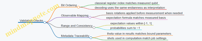
7. Post-processing and validation checks that outputs match the assumptions you made earlier, such as bit ordering and observable mapping.

If you treat each stage as a boundary with explicit inputs and outputs, debugging becomes less like detective work and more like following a checklist.

Mind Map: End-to-End Flow

Concrete Example: From a Parameterized Circuit to an Expectation Value

Suppose you want the expectation value of a single-qubit observable \(Z\) for a state prepared by a rotation \(R_y(\theta)\). In a measurement-based pipeline, the key is that “what you measure” and “what you compute” must agree.

Example: Logical Circuit and Measurement Meaning

• Logical circuit: apply \(R_y(\theta)\) to qubit 0.
• Measurement: measure qubit 0 in the computational basis.
• Interpretation: compute \(\langle Z \rangle = P(0) - P(1)\).

If your code accidentally flips bit order or interprets the wrong classical register, you’ll get a consistent but incorrect value. That’s why validation belongs at the end.

Minimal Pseudocode for the Pipeline

# 1) Design logical circuit (conceptual)
# circuit(theta): apply Ry(theta) on qubit 0, then measure qubit 0

# 2) Bind parameters for this run
bound = bind_parameters(circuit, {"theta": 1.234})

# 3) Compile to backend constraints
compiled = compile_for_backend(bound, backend_config)

# 4) Package and execute
job = submit_job(compiled, shots=2000, metadata={"theta": 1.234})
raw = job_result(job)  # raw counts or samples

# 5) Interpret results into expectation value
p0 = raw.counts["0"] / 2000
p1 = raw.counts["1"] / 2000
exp_z = p0 - p1

# 6) Validate assumptions
assert -1.0 <= exp_z <= 1.0

What “Mapping” Really Means: Measurement Semantics

The most common workflow mistake is assuming that measurement semantics survive every transformation automatically. Compilation may reorder qubits, insert swaps, or rewrite gates. A robust mapping strategy is to:

• Name the measurement intent in the logical circuit, such as “classical bit 0 corresponds to qubit 0’s Z measurement.”
• Track qubit-to-classical-bit mapping through compilation and result decoding.
• Validate with a known input: for example, if you prepare \(|0\rangle\), then \(\langle Z \rangle\) should be near +1 (up to noise and finite shots).

Mind Map: Validation Checks

Practical Takeaway

When you map circuit design to results, you’re really mapping meaning. Gates are instructions, but measurement semantics are the contract that turns those instructions into numbers you can trust.

1.2 Defining the Hybrid Boundary Between Classical and Quantum Components

A hybrid application is easiest to reason about when you can point to a clear “contract boundary”: what the classical side decides, what the quantum side computes, and what data crosses the line. The boundary is not just architectural; it determines correctness, performance, and how you test the program.

What Stays Classical

Keep these responsibilities on the classical side:

• Control flow and orchestration: loops, batching, retries, and selecting which circuits to run next.
• Parameter management: storing parameter values, validating shapes, and mapping optimizer variables to circuit parameters.
• Result interpretation: converting raw measurement data into expectation values, losses, and gradients.
• Data integrity checks: verifying that the returned results match the requested circuit identity and shot count.

A practical rule: if the logic can be unit-tested without a quantum backend, it belongs to classical code.

What Stays Quantum

Keep these responsibilities on the quantum side:

• State preparation and circuit evolution: building the circuit that maps inputs to measurement statistics.
• Measurement generation: defining which qubits are measured and how outcomes are encoded.
• Observable sampling: when you need basis rotations or structured measurement patterns, the circuit should express that.

A practical rule: if the logic depends on gate-level structure or measurement layout, it belongs to the quantum circuit.

The Boundary Contract

Define a small set of inputs and outputs that cross the boundary.

• Inputs: a parameter vector (or a small structured object), plus a circuit identifier.
• Outputs: either counts/bitstrings or expectation values with enough metadata to interpret them.

If you only pass parameters and receive counts, you keep the boundary simple and framework-agnostic. If you pass expectation values, you must standardize how each framework computes them.

Mind Map: Hybrid Boundary Decisions

Example: A Clean Boundary for a Variational Loop

In this pattern, the classical code owns the optimizer and the quantum code owns the circuit. The boundary passes parameters in, counts out.

# Classical side: orchestration and interpretation
def evaluate_loss(params, circuit_id, run_quantum):
    counts, meta = run_quantum(circuit_id, params)
    # Example: compute <Z> on qubit 0 from counts
    shots = meta["shots"]
    p0 = sum(v for b, v in counts.items() if b[-1] == "0") / shots
    p1 = 1 - p0
    exp_z = p0 - p1
    return 1 - exp_z

The quantum runner can be framework-specific, but it must obey the same contract: return counts keyed by bitstrings and include shots.

Example: When Expectation Values Cross the Boundary

Sometimes you want the quantum side to return expectation values directly. That can reduce classical code, but it increases coupling because you must standardize measurement conventions.

# Quantum side contract variant: expectation value returned
# exp_value is computed from the measurement circuit
# meta includes measurement basis and qubit mapping

def run_quantum_expectation(circuit_id, params):
    exp_value, meta = backend_execute_and_postprocess(circuit_id, params)
    return exp_value, meta

If you choose this variant, the classical side should treat meta as mandatory input for correctness checks, not optional decoration.

Boundary Pitfalls to Avoid

• Hidden parameter binding: if parameter names differ between circuit construction and execution, you can silently evaluate the wrong circuit.
• Unspecified bit ordering: bitstrings may be reversed depending on conventions, so define how qubit indices map to string positions.
• Mixing concerns in post-processing: if basis-rotation logic lives partly in the circuit and partly in classical code, tests become harder.

A Simple Checklist for Defining the Boundary

• Can you describe the boundary with one sentence: “classical passes X, quantum returns Y”?
• Are the data types stable: parameter vector in, counts out (or expectation out) with required metadata?
• Can you unit-test the classical interpretation using synthetic counts?
• Can you validate the quantum circuit structure without running it?

When these answers are “yes,” your hybrid program becomes easier to test and easier to modify without breaking the meaning of results.

1.3 Choosing the Right Abstractions for Circuits, Experiments, and Jobs

A quantum software stack usually has three layers that people mix up: the circuit (what you want), the experiment (how you measure it), and the job (how you run it). Choosing the right abstraction for each layer keeps your code readable and your results trustworthy.

Circuits: The “What” With Structure

A circuit is a structured description of quantum operations: qubits, gates, parameters, and measurement instructions. Treat it like a reusable artifact. If you find yourself changing measurement logic every time you run the same algorithm, you probably put too much into the circuit.

Best practice: keep circuits focused on state preparation and unitary structure, and make measurement explicit but minimal. For example, you can build a parameterized ansatz circuit once, then reuse it across multiple measurement strategies.

Example: a parameterized circuit that prepares a state for an energy estimator.

# Qiskit-style pseudocode
from qiskit import QuantumCircuit

def ansatz(theta):
    qc = QuantumCircuit(2)
    qc.ry(theta[0], 0)
    qc.cx(0, 1)
    qc.ry(theta[1], 1)
    return qc

Here, the circuit describes the state preparation. It does not decide how many shots to use, which backend to target, or how to post-process counts.

Experiments: The “How” With Measurement Semantics

An experiment packages a circuit with measurement intent: what observable you’re estimating, how you map observables to measurement bases, and how you interpret raw outcomes. In practice, experiments often include:

• A measurement plan (basis rotations, ancilla usage, or observable term grouping)
• A sampling configuration (shots) or an estimator configuration
• A result schema (counts, quasi-distributions, expectation values)

Best practice: treat experiments as the unit you vary when you change measurement strategy. If you switch from measuring Z on each qubit to measuring an X⊗Z observable, that change belongs in the experiment layer.

Example: two experiments that reuse the same ansatz but estimate different observables.

# Conceptual pseudocode
# Experiment A: measure Z on qubit 0
# Experiment B: measure X on qubit 0

experiment_A = {
  "circuit": ansatz(theta),
  "measurement": "Z on q0",
  "shots": 2000
}

experiment_B = {
  "circuit": ansatz(theta),
  "measurement": "X on q0",
  "shots": 2000
}

Even if the underlying framework hides basis rotations, the abstraction boundary still helps you reason about what changed.

Jobs: The “Where and When” With Execution Control

A job represents an execution request: target backend or simulator, runtime options, batching behavior, and the lifecycle from submission to results. Jobs are where you handle operational concerns like:

• Backend selection and constraints
• Transpilation or compilation settings
• Timeout, retries, and result retrieval
• Metadata for traceability

Best practice: keep jobs thin. They should not contain algorithm logic. If you need to change algorithm behavior, you should update the circuit or experiment, then create a new job.

Example: running the same experiment on two backends.

# Qiskit-style pseudocode
# job_sim = backend_sim.run(experiment)
# job_hw  = backend_hw.run(experiment)

job_sim = submit_job(experiment_A, backend="simulator")
job_hw  = submit_job(experiment_A, backend="hardware")

The circuit and experiment remain the same; only the execution context changes.

Mind Map: How the Layers Fit Together

A Practical Rule for Picking the Layer

Ask one question: “If I change this requirement, what should I rebuild?”

• Change the ansatz structure or parameters: rebuild the circuit.
• Change what you measure or how you interpret outcomes: rebuild the experiment.
• Change where/how you run: rebuild the job.

This rule prevents a common bug: accidentally reusing a job result with the wrong measurement interpretation. When the experiment layer owns measurement semantics, your post-processing code can validate that it matches the experiment schema.

Example: A Clean Hybrid Loop Boundary

In a hybrid optimization loop, the classical optimizer proposes parameters. The stack should then:

1. Bind parameters into the circuit (circuit layer).
2. Create or select an experiment that defines the observable and measurement plan (experiment layer).
3. Submit a job to a backend with the chosen execution options (job layer).

Keeping these steps separate makes it easier to debug. If results look wrong, you can check whether the circuit binding is correct, whether the experiment’s measurement plan matches the intended observable, or whether the job ran with the expected settings.

1.4 Practical Data Flow Contracts for Inputs, Parameters, and Measurement Outputs

Hybrid quantum programs fail in predictable ways: the circuit is correct, but the inputs are mis-bound, the parameters are swapped, or the measurement outputs are interpreted with the wrong bit order. A data flow contract is the small set of rules that prevents those failures. It specifies what each function accepts, what it returns, how parameters are represented, and how measurement results are decoded.

Data Flow Contract Goals

A good contract makes three things explicit. First, it defines the shape of inputs so classical code can validate before submitting quantum work. Second, it defines how parameters are named, typed, and bound so the same logical parameter means the same physical value across runs. Third, it defines how measurement outputs are represented so post-processing is consistent with the circuit’s measurement convention.

Mind Map: Data Flow Contract Components

Inputs Contract

Treat every quantum call like a function with a signature. For example, define an input payload with fields for classical features and optional metadata.

Contract rules

• The feature vector has a fixed length per circuit family.
• Values are numeric and finite; reject NaN and infinities before building circuits.
• The contract states whether features are normalized or not, so you don’t “fix” them twice.

Easy example

• You build a circuit that expects x = [x0, x1] and uses them as rotation angles.
• Your classical wrapper checks len(x) == 2 and that all values are finite.
• If the check fails, you raise a clear error before any quantum job is created.

Parameters Contract

Parameters are where silent bugs breed. The contract should define a naming scheme and a binding strategy.

Contract rules

• Parameter names are stable strings like theta_0, theta_1, not positional indices.
• The binding method is explicit: either a dictionary mapping names to values, or a list with a documented order.
• The contract defines whether parameters are angles in radians and whether they are wrapped to a range.

Easy example

• A variational circuit uses parameters theta_0 and theta_1.
• The classical optimizer produces a vector [t0, t1].
• Your binding step maps theta_0 -> t0 and theta_1 -> t1 using a dictionary, not by assuming the circuit’s internal parameter order.

Measurement Outputs Contract

Measurement outputs must be decoded with the same bit ordering used when the circuit measured qubits. The contract should define an output schema that post-processing can rely on.

Contract rules

• The output includes shots and either counts or an explicit list of measured bitstrings.
• The contract defines bit ordering: for instance, “leftmost bit corresponds to qubit 0” or the opposite.
• If you compute expectation values, the contract states the observable’s mapping from bitstrings to eigenvalues.

Easy example

• Suppose qubits [q0, q1] are measured and you receive bitstrings like 00, 01, 10, 11.
• If your post-processing assumes q0 is the leftmost bit but the backend returns the rightmost bit as q0, your expectation value flips in a way that looks like a real signal.
• The contract prevents this by forcing a single documented convention and a conversion step when needed.

Practical Output Schema

Use a small, consistent structure for results. Even if you later add more fields, keep the core stable.

Example: Contract-Driven Wrapper

This wrapper validates inputs, binds parameters by name, and normalizes measurement outputs into a schema.

def run_hybrid(payload, circuit_builder, executor):
    x = payload["features"]
    params = payload["parameters"]  # dict name->float

    if len(x) != circuit_builder.feature_dim:
        raise ValueError("Feature vector has wrong length")
    for v in x:
        if not (isinstance(v, (int, float)) and v == v and abs(v) != float('inf')):
            raise ValueError("Feature vector contains non-finite values")

    circuit, param_names = circuit_builder.build()
    if set(params.keys()) != set(param_names):
        raise ValueError("Parameter names mismatch")

    bound = circuit.bind_parameters(params)
    raw = executor.submit(bound)

    return normalize_counts(raw, bit_order="q0_left")

Mind Map: Measurement Normalization Steps

Contract Checks for Post-Processing

Post-processing should also be contract-driven. Before computing an expectation value, verify that the counts keys match the expected bitstring length and that shots equals the sum of counts. If not, stop and report the mismatch. That single check saves hours of debugging when a circuit changes but the decoding code doesn’t.

Summary Rules

A practical contract is small but strict: validate input shapes and finiteness, bind parameters by stable names, normalize measurement outputs into a documented bit ordering, and verify result schemas before computing any derived quantities.

1.5 Reproducibility Requirements for Deterministic Runs and Traceability

Reproducibility in hybrid quantum software means that the same inputs produce the same outputs, or at least the same outputs within a clearly stated tolerance. In practice, you rarely get perfect determinism because sampling, noise, and backend behavior introduce randomness. The goal is to make randomness explicit, record enough context to rerun, and validate that reruns behave the same way.

Define Determinism Levels

Not all parts of a hybrid pipeline need the same determinism.

• Circuit determinism: The circuit structure, parameter values, and measurement mapping are identical across runs.
• Execution determinism: The simulator or backend uses a fixed seed and consistent execution settings.
• Statistical determinism: Results match within expected sampling error, given the same shot budget and noise model.

A useful rule: if you cannot explain why two runs differ, you do not yet have reproducibility.

Capture a Run Manifest

A run manifest is a compact record of everything that affects results. Treat it like a receipt: it should be readable by humans and machine-checkable.

Include:

• Code version: commit hash or package versions.
• Framework versions: Qiskit and Cirq versions, plus Cirq version.
• Backend identity: backend name, target device, and any configuration knobs.
• Execution settings: shot count, optimization level, transpilation options, and any seed values.
• Circuit identity: a stable circuit hash, plus parameter values bound for the run.
• Measurement mapping: qubit-to-bit ordering and any basis rotation operations.
• Noise configuration: noise model parameters or simulator noise flags.
• Runtime metadata: timestamps, job IDs, and any result-processing version.

Use Stable Identifiers for Circuits and Parameters

Circuit objects can be hard to compare directly. Instead, compute a stable representation.

• Serialize the circuit to a canonical form (same gate ordering rules, same parameter naming).
• Hash the serialized form to get a circuit_id.
• Store parameter_bindings as an ordered mapping from parameter names to numeric values.

This prevents “same idea, different representation” bugs, like binding parameters in a different order or changing measurement bit order.

Control Randomness Explicitly

Randomness enters through sampling and sometimes through transpilation or simulator internals.

• Simulator seeds: set them for both frameworks when supported.
• Sampling seeds: if the sampler API supports it, set it.
• Classical randomness: seed optimizers, initial guesses, and any data shuffling.

If a component does not support seeding, record that fact in the manifest and rely on statistical determinism checks.

Validate Traceability with Round-Trip Checks

Traceability means you can reconstruct the run from the manifest.

Perform a round-trip:

1. Build the circuit from your source algorithm.
2. Bind parameters from the manifest.
3. Re-run with the same execution settings.
4. Compare circuit_id and measurement mapping.
5. Compare results using a metric appropriate for the task.

For example, if you compute an expectation value from counts, compare the expectation and its uncertainty rather than requiring identical raw counts.

Mind Map: Reproducibility and Traceability

Example: Minimal Run Manifest for a Hybrid Evaluation

{
  "run_id": "2026-03-31T10:15:22Z_7f3a",
  "code_commit": "a1b2c3d",
  "qiskit_version": "1.x.y",
  "cirq_version": "1.x.y",
  "backend": {"name": "qasm_simulator", "target": "local"},
  "execution": {
    "shots": 20000,
    "seed": 12345,
    "transpile_optimization_level": 2
  },
  "circuit": {
    "circuit_id": "sha256:...",
    "parameter_bindings": {"theta": 0.314159, "phi": 1.2},
    "measurement_mapping": {"qubit": [0,1], "bit": [0,1]}
  },
  "noise": {"model": "none"},
  "result_processing": {"version": "1.0.0"}
}

Example: Deterministic Circuit, Statistical Results

Suppose you run a circuit that prepares a known state and measures in the computational basis. With the same circuit_id, parameter_bindings, and measurement mapping, the expectation value should be close to the theoretical value. With fixed seeds and a simulator, you may get identical counts. With hardware or noise sampling, you should instead check that the expectation value lies within an uncertainty band computed from shot noise.

A practical comparison approach:

• Compute expectation value and standard error from counts.
• Require the rerun’s expectation to fall within, say, 2 standard errors of the original.
• If it fails, treat it as a reproducibility issue and inspect manifest fields first: shots, seeds, measurement mapping, and noise settings.

Reproducibility is not a single switch. It is a set of agreements: what must match exactly, what may vary but should vary predictably, and how you prove both through recorded context and validation checks.

2.1 Qubit Indexing, Register Layout, and Measurement Conventions

Qubit indexing is where “what you meant” meets “what the compiler did.” A consistent convention prevents silent mismatches between circuit construction, transpilation, and measurement post-processing.

Qubit Indexing Models

Most frameworks let you refer to qubits by integer index, but the meaning of that index depends on how you build registers.

• Single register indexing: Qubits are numbered 0..n-1 in the order you created the register. Measurement results typically follow the same order.
• Multiple register indexing: You may have separate registers (e.g., data and ancilla). Frameworks usually flatten them into one global index. The flattening order is defined by register creation order and sometimes by framework-specific conventions.
• Explicit mapping: Some APIs allow you to map logical qubits to physical qubits or to specify a layout. This is the safest approach when you expect transpilation or hardware constraints to reorder things.

A practical rule: decide whether your code treats indices as logical (meaning inside the algorithm) or physical (meaning on a device). Then keep that meaning stable across the whole pipeline.

Register Layout and Flattening

When you have multiple registers, you need to know how they become a single measurement bitstring.

Consider a circuit with two registers:

• data has 2 qubits: indices 0 and 1 (logical)
• ancilla has 1 qubit: index 2 (logical)

If the framework flattens registers in creation order, then global indices are [data[0], data[1], ancilla[0]]. If it flattens in a different order, your measurement bitstring will be permuted.

To avoid guessing, treat the mapping as data. Print or inspect the circuit’s qubit ordering right before execution, and use that ordering when you interpret results.

Measurement Bitstring Conventions

Measurement produces classical bits, and classical bits are often packed into a bitstring. Two conventions matter:

1. Bit order within the string: Many systems present the most significant bit first, but some interpret index 0 as the least significant bit. This affects how you read outcomes like 010.
2. Which qubit maps to which classical bit: Measurement can be attached to specific classical registers or to a single classical register. The mapping determines which measured qubit corresponds to which position in the output.

A good habit is to test with a circuit that prepares a known computational basis state. If you expect qubit 0 to be 1 and you see the 1 in a different position, you’ve found a convention mismatch.

Example: Known State Sanity Check

Here’s a minimal sanity check idea: prepare a basis state by applying X gates, measure all qubits, and verify the bitstring position.

# Pseudocode-style example
# Prepare |q0 q1 q2> = |1 0 1>
# Then measure all qubits and interpret the bitstring.

# 1) Apply X to q0 and q2
# 2) Measure q0, q1, q2 into a classical register
# 3) Run once (or with few shots)
# 4) Confirm that the output bitstring encodes 1-0-1

If the bitstring does not match your expected ordering, do not “fix” it by trial and error in the optimizer loop. Fix it once in your measurement interpretation function.

Mind Map: Indexing and Measurement

Mind Map: Qubit Indexing and Measurement Conventions

Example: Centralized Decoding Function

Instead of scattering bitstring decoding logic across the codebase, centralize it. The function should accept the raw bitstring and return a dictionary like {qubit_index: bit_value}.

# Pseudocode-style example

def decode_measurement(bitstring, qubit_order):
    # qubit_order: list of qubit indices in the order
    # that the framework packs bits into the string.
    # Return mapping qubit -> measured bit.
    mapping = {}
    for pos, q in enumerate(qubit_order):
        mapping[q] = int(bitstring[pos])
    return mapping

The key is that qubit_order is derived from the circuit’s actual qubit ordering, not from your assumptions.

Practical Checklist

• Use one consistent convention for logical qubit indices.
• Know how registers flatten into global indices.
• Confirm bitstring order with a known basis-state test.
• Centralize measurement decoding so the optimizer never touches raw bitstrings.
• Inspect qubit ordering right before execution, especially after transpilation or layout changes.

2.2 Gate Decomposition Rules and How Software Represents Them

Gate decomposition is the process of rewriting a circuit so every operation fits a target gate set and hardware constraints. Software does this in a way that preserves the circuit’s meaning: the same unitary effect (up to numerical tolerance), the same measurement semantics, and the same parameter mapping.

What “Decomposition” Means in Practice

A decomposition pass typically takes three inputs: (1) an input circuit with gates and parameters, (2) a target basis gate set, and (3) constraints such as coupling maps or allowed directions. The output is a new circuit where each original gate is replaced by a sequence of basis gates, and where any required swaps or routing operations are inserted to satisfy connectivity.

A key rule: decomposition should not change classical control flow. If a circuit uses conditional operations based on measurement results, those conditions must remain attached to the correct logical qubits, even if the quantum operations around them are rewritten.

Representation: From “Gates” to “Operations”

Most quantum SDKs represent circuits as a list of operations with metadata. Each operation includes:

• The gate type (e.g., Hadamard, controlled-NOT, rotation)
• The qubit targets (which wires it acts on)
• Optional parameters (angles, symbols)
• Optional classical conditions (e.g., apply only if a register equals a value)
• Timing or ordering information (explicit moments or implicit depth)

Decomposition works by pattern-matching gate types and then emitting replacement operations. For parameterized gates, the replacement must reuse the same parameter symbols so later binding still works.

Core Decomposition Rules

Single-Qubit Gates Decompose into Basis Rotations

If the target basis contains rotations like Rx, Ry, Rz, then any single-qubit unitary can be expressed as a product of rotations plus a global phase. Software usually chooses a canonical decomposition so that repeated runs produce stable circuits.

Example: Suppose the basis is {Rx, Ry, Rz}. A Hadamard gate H can be rewritten using rotations. One common identity is:

• H ≈ Rz(π) · Rx(π/2) · Rz(π)

The approximation is exact up to global phase, which measurement probabilities ignore.

Controlled Gates Decompose Using Ancilla-Free Patterns When Possible

For a controlled-U gate, software often uses a standard decomposition into controlled rotations and single-qubit rotations. If the basis includes a native controlled-NOT, it may further reduce the controlled-U into CNOT plus single-qubit gates.

Example: If the basis is {CNOT, Rx, Ry, Rz}, then a controlled-Ry(θ) can be implemented with two CNOTs and rotations on the control/target wires. The exact sequence depends on the chosen convention, but the rule is consistent: the control condition is enforced by entangling operations that only touch the control and target qubits.

Two-Qubit Gates Decompose into Basis Two-Qubit Primitives

When the basis includes only one kind of two-qubit gate (often CNOT), general two-qubit unitaries are decomposed into a sequence of that primitive plus single-qubit rotations. Many SDKs use a canonical form to ensure the same input gate yields the same decomposition structure.

Example: A generic controlled-phase gate CZ can be expressed as:

• CZ = H on target · CNOT · H on target

This is a useful decomposition rule because it preserves the logical meaning while translating into a basis the backend can execute.

Connectivity Constraints Insert Routing Operations

If qubits are not directly connected, decomposition adds SWAP operations (or equivalent routing) to move quantum states so that required two-qubit gates can occur. The rule is: routing changes the mapping between logical and physical qubits, so software must track that mapping throughout the circuit.

Example: If logical qubits q0 and q2 need a CNOT but only q0–q1 and q1–q2 couplings exist, the compiler may insert SWAP(q1,q2) before the CNOT and then swap back afterward, depending on the optimization strategy.

Mind Map: Decomposition Pipeline and Responsibilities

Gate Decomposition Mind Map

Example: Parameterized Gate Decomposition with Symbol Preservation

Consider a circuit fragment with a symbolic parameter θ:

• Apply Rx(θ) on q0
• Apply CNOT from q0 to q1

If the target basis is {Rz, Ry, CNOT}, software may rewrite Rx(θ) into a sequence of Rz and Ry gates using identities that keep θ as a symbol. The decomposition must not replace θ with a numeric value during compilation; otherwise later binding would break.

A practical sanity check is to inspect the emitted circuit and confirm that the parameter appears in the replacement operations exactly as a symbol, not as a computed float.

Validation Rules That Prevent Subtle Bugs

After decomposition, software should run checks that are cheap but effective:

• No unsupported gate types remain in the circuit.
• All classical conditions still reference the same logical qubits as before.
• Parameter symbols are present and consistently named.
• For routing, the final logical-to-physical mapping matches the expected outcome for subsequent operations.

When these checks pass, decomposition is doing its job: translating gate semantics into a form the backend can execute without changing what the circuit is supposed to measure.

2.3 Circuit Depth, Connectivity Constraints, and Scheduling Implications

Circuit depth is the number of sequential “time steps” your quantum program needs, assuming gates that act on different qubits can run in parallel. In practice, depth is shaped by two things: (1) how your circuit is written and (2) what the target device can physically do. When you move from an ideal circuit to a real backend, the compiler often inserts extra operations, especially SWAPs, to satisfy connectivity constraints. Those inserted operations increase both depth and the total number of noisy opportunities.

Depth as a Software-Visible Metric

A useful mental model is to treat each qubit as a timeline. A gate occupies a time slot on each qubit it touches. If two gates touch disjoint qubits, they can share the same slot. If they touch the same qubit, they must be ordered. This means depth is not just “how many gates exist,” but “how they overlap across qubits.”

A quick check: if your circuit has many two-qubit gates that all involve the same qubit, depth will grow even if the gate count is modest. Conversely, if your two-qubit gates form layers that touch different qubit pairs, depth can stay relatively low.

Connectivity Constraints and Why SWAPs Appear

Most hardware does not allow arbitrary two-qubit interactions. Instead, it supports interactions only along edges of a coupling graph. If your circuit requests a two-qubit gate between qubits that are not connected, the compiler must move quantum state around the device until the requested pair becomes adjacent.

That “moving” is typically done with SWAP operations. A SWAP is not free: it adds depth and consumes additional gates, which matters because noise accumulates with the number of operations.

Mind Map: Depth Drivers and Constraint Effects

Scheduling Implications in Concrete Terms

Scheduling is the compiler’s job of assigning gates to time slots while respecting dependencies and device constraints. Even if two gates are logically independent, scheduling may delay one because of limited connectivity or because a qubit is already busy.

A common pattern: your circuit is written as a neat sequence of two-qubit gates, but the device coupling graph forces the compiler to route states. Routing creates additional dependencies, because SWAPs move states and therefore change which logical qubit resides on which physical qubit at each step.

This is why “depth inflation” can happen: the compiler is not just adding SWAPs; it is also creating new ordering constraints.

Example: A Simple Connectivity Clash

Suppose the device supports two-qubit gates only between neighboring qubits in a line: (0–1), (1–2), (2–3). Your circuit asks for a two-qubit gate between qubits 0 and 3.

• Logical request: gate(0, 3)
• Physical reality: 0 and 3 are not adjacent
• Typical compiler response: move state from 0 toward 3 using SWAPs, apply the gate, then move state back if needed.

Even without writing the exact sequence, you can reason about depth impact. Any route from 0 to 3 on a line requires at least two SWAP “hops” in one direction, and often more depending on whether the compiler keeps states permuted or restores them. Each hop is a time step, and the gate itself adds another.

Example: Layering to Reduce Depth

Consider four qubits with a coupling graph that supports interactions between (0–1) and (2–3) but not across those pairs. If you schedule two-qubit gates as two separate layers—first apply gate(0,1) and gate(2,3) simultaneously, then apply gate(1,2) later—you get better parallelism than if you interleave them in a way that forces qubits to wait.

The key is to group gates into layers where each qubit participates in at most one gate per layer. When you do this, the compiler has fewer opportunities to create unnecessary serialization.

Practical Best Practices for Depth and Scheduling

1. Prefer hardware-friendly gate patterns. If your algorithm naturally expresses interactions in a local pattern, keep it local in the circuit. When you must use long-range interactions, expect routing overhead.
2. Check for “hot” qubits. If one qubit participates in many two-qubit gates, depth will likely grow quickly. Restructuring the circuit to distribute interactions can reduce serialization.
3. Use parameter binding instead of rebuilding circuits. Rebuilding can hide scheduling opportunities and makes it harder to compare depth across iterations. Binding keeps the structure stable.
4. Inspect the compiled circuit, not just the source. The compiled output reveals where SWAPs and decompositions were inserted, which directly explains depth changes.

Mind Map: Scheduling Workflow

Depth, connectivity, and scheduling are tightly linked: connectivity constraints force state movement, state movement creates new dependencies, and those dependencies determine how many time steps the final circuit needs. If you treat depth as a first-class design metric, you can often reduce the amount of routing the compiler must do, which usually means fewer operations and cleaner execution.

2.4 Parameterized Circuits and Binding Strategies in Practice

Parameterized circuits let you build one circuit “skeleton” and reuse it with different numeric values. The trick is to keep the parameter mapping unambiguous from circuit construction through execution and result interpretation.

Parameter Kinds and Where They Live

In both Qiskit and Cirq, parameters are placeholders that get replaced later. The practical difference is how they are represented and when they are resolved.

• Symbolic parameters represent unknown values during circuit construction.
• Bound parameters are concrete numbers used during execution.
• Bound-at-build vs bound-at-run determines whether you create a new circuit object per parameter set or reuse the same circuit with a binding step.

A good rule: if you will evaluate many parameter sets, prefer binding at run time so you avoid rebuilding the circuit graph repeatedly.

Mind Map: Parameterization and Binding

Binding Strategies That Don’t Surprise You

Strategy 1: Bind by Name, Not by Position

When you bind multiple parameters, position-based binding can silently mis-map values if the parameter order changes. Name-based binding keeps the mapping explicit.

Example: Suppose you have parameters theta and phi. If you accidentally swap them, the circuit still runs but the results correspond to a different model.

Strategy 2: Keep a Single Parameter Schema

Define parameters once and reuse them across circuit components. If you create new parameter objects with the same label, you may end up binding the wrong placeholders.

Strategy 3: Separate Circuit Construction from Binding

Build the circuit with symbolic parameters only. Then create a binding dictionary or resolver at execution time. This separation makes it easier to test that the circuit structure is correct before you start worrying about numeric values.

Qiskit Example: One Circuit, Many Bindings

Below, the circuit is constructed once. Each binding produces a new parameter assignment without changing the circuit topology.

from qiskit import QuantumCircuit
from qiskit.circuit import Parameter

theta = Parameter("theta")
phi = Parameter("phi")

qc = QuantumCircuit(2)
qc.ry(theta, 0)
qc.rz(phi, 0)
qc.cx(0, 1)

bindings = [
    {theta: 0.1, phi: 0.2},
    {theta: 1.0, phi: -0.5},
]

# Later: pass bindings to your execution path
# Example: sampler.run([(qc, bindings[i]) for i in range(len(bindings))])

If you later add a third parameter, you update the schema in one place and the binding dictionaries become the single source of truth.

Cirq Example: Resolver-Based Binding

Cirq uses a resolver concept to map symbols to values. The key is that the resolver must include every symbol used by the circuit.

import sympy
import cirq

theta, phi = sympy.symbols('theta phi')

q0, q1 = cirq.LineQubit.range(2)

circuit = cirq.Circuit(
    cirq.ry(theta)(q0),
    cirq.rz(phi)(q0),
    cirq.CNOT(q0, q1),
)

resolvers = [
    cirq.ParamResolver({theta: 0.1, phi: 0.2}),
    cirq.ParamResolver({theta: 1.0, phi: -0.5}),
]

# Later: execute with each resolver

A missing symbol is a common failure mode. Treat “all parameters must be bound” as a hard requirement in your execution wrapper.

Binding Correctness Checks

Before running expensive experiments, validate that your binding step is consistent.

• Parameter coverage: every circuit symbol must appear in the binding map.
• No extra keys: bindings should not contain unrelated parameters.
• Deterministic mapping: the same binding dictionary should always produce the same resolved circuit.

A simple invariant test is to resolve the circuit twice with the same binding and compare the resolved gate parameters. If they differ, your binding pipeline is not stable.

Practical Guidance for Hybrid Loops

In hybrid optimization loops, you typically evaluate many parameter sets. Use binding strategies that keep circuit construction out of the inner loop. Store parameter schemas and binding dictionaries in a consistent format so your classical code can generate bindings without guessing parameter order. When you do this, the quantum part becomes a predictable function: inputs are parameter values, outputs are measurement-derived numbers.

2.5 Validating Circuit Structure with Static Checks and Invariant Tests

Circuit bugs are often boring: a qubit index off by one, a measurement placed on the wrong wire, or a parameter left unbound. Static checks catch these issues before you run anything; invariant tests confirm that the circuit behaves the way you think it does, even after refactors.

Static Checks That Fail Fast

Static checks operate on the circuit object without executing it. They should be cheap, deterministic, and strict.

1) Register and wire consistency

• Verify that every gate targets an existing qubit index.
• Verify that every measurement maps to a valid classical bit index.
• In Qiskit, confirm that the number of qubits in the circuit matches the backend or simulator expectations you plan to use.

2) Measurement placement rules

• Decide a policy: either measurements appear only at the end, or you allow mid-circuit measurements with explicit handling.
• Enforce the policy by scanning operations in order and flagging forbidden patterns.

3) Parameter binding completeness

• For parameterized circuits, ensure that every parameter has a value before execution.
• If you support partial binding, define which parameters may remain symbolic and how they will be resolved later.

4) Gate shape and arity

• Validate that each operation has the correct number of targets.
• For example, a two-qubit gate must reference exactly two distinct qubits.

5) Deterministic canonicalization for comparisons

• When you compare circuits in tests, normalize representation so that equivalent circuits don’t fail due to ordering differences.
• A simple approach is to compare a canonical “signature” you compute from operations and their targets.

Invariant Tests That Confirm Meaning

Invariant tests check properties that should hold regardless of how the circuit was constructed.

Invariant A: Circuit signature stability If you build a circuit from a known specification, the resulting operation list should match a stable signature.

Invariant B: Measurement semantics Given a known input state (or a known simulator setting), the measurement distribution should match expectations within tolerance.

Invariant C: Parameter substitution correctness Substituting parameters should not change the circuit structure beyond replacing symbolic values.

Invariant D: No accidental wire swaps For circuits that are supposed to act on specific qubits, verify that swapping indices changes the signature in the expected way, not silently.

Mind Map: Validation Strategy

Mind Map: Circuit Validation

Example: Qubit and Measurement Index Validation

Here’s a minimal pattern for static validation. The goal is to raise a clear error before execution.

def validate_indices(num_qubits, num_clbits, ops):
    for op in ops:
        for q in op.get('qubits', []):
            if q < 0 or q >= num_qubits:
                raise ValueError(f"Invalid qubit index {q}")
        for c in op.get('clbits', []):
            if c < 0 or c >= num_clbits:
                raise ValueError(f"Invalid classical bit index {c}")

Use this idea by extracting an operation list from your circuit representation (Qiskit or Cirq) into a uniform structure for validation.

Example: Enforcing End-Only Measurements

If your application assumes measurements happen at the end, enforce it.

def validate_end_only_measurements(ops):
    seen_measure = False
    for i, op in enumerate(ops):
        is_meas = op['type'] == 'measure'
        if is_meas:
            seen_measure = True
        elif seen_measure:
            raise ValueError(f"Gate after measurement at position {i}: {op['type']}")

This catches a common refactor mistake: inserting a diagnostic measurement and forgetting to remove it.

Example: Invariant Test for Parameter Substitution

A good invariant test checks that substitution changes only parameter values, not targets or gate types.

def signature(circuit):
    return [(op['type'], tuple(op.get('qubits', [])), tuple(op.get('clbits', [])))
            for op in circuit['ops']]

def test_parameter_substitution_structure(original, substituted):
    assert signature(original) == signature(substituted)

To make this meaningful, ensure your “signature” includes enough structure to detect accidental wire swaps and missing targets.

Example: Measurement Semantics Test on a Known Circuit

For a simple circuit, you can test measurement semantics directly. For instance, a circuit that prepares \(|0\rangle\) and measures should produce only bit 0 (up to simulator noise settings).

A practical approach is:

• Use a simulator mode with deterministic behavior when possible.
• Compare the observed distribution to the expected one with a tolerance.
• Fail with the top mismatched outcomes so debugging is fast.

Failure Messages That Help

When validation fails, include:

• The operation index in the circuit.
• The offending qubit or classical bit index.
• The operation type.

A failure that says “invalid qubit index 7” is useful; one that says “something went wrong” is not. Static checks and invariant tests work best when they point directly at the mistake you can fix in minutes, not hours.

3.1 Building Circuits With QuantumCircuit and Register Management

A circuit is only as clear as its wiring and naming. In Qiskit, that clarity starts with registers: you decide how many qubits exist, how they are grouped, and how measurement results map back to classical bits. The goal is simple: when you later read counts or build a parameterized circuit, you should not have to guess which bit came from which qubit.

Register Types and Why They Matter

Qiskit uses two main register categories:

• Quantum registers hold qubits. Their indices define where gates apply.
• Classical registers hold measurement results. Their indices define where bits land.

A common best practice is to keep register sizes explicit and stable. If you later change the number of qubits, you want failures to happen early (during construction) rather than silently producing wrong measurement mappings.

A Minimal Circuit with Explicit Registers

This example creates two qubits and one classical register of two bits, then measures each qubit into the corresponding classical bit.

from qiskit import QuantumCircuit, QuantumRegister, ClassicalRegister

q = QuantumRegister(2, "q")
c = ClassicalRegister(2, "c")

qc = QuantumCircuit(q, c)
qc.h(q[0])
qc.cx(q[0], q[1])
qc.measure(q, c)

print(qc)

The line qc.measure(q, c) measures qubit q[0] into c[0] and q[1] into c[1]. That one-to-one mapping is the foundation for interpreting bitstrings later.

Mind Map: Registers and Measurement Mapping

Mind Map: QuantumCircuit Registers and Measurement

Partial Measurement and Intentional Bit Placement

Sometimes you only need a subset of qubits, or you want results stored in a specific classical layout. Use explicit mapping to avoid accidental swaps.

from qiskit import QuantumCircuit

qc = QuantumCircuit(3, 2)
qc.x(2)          # put a known state on qubit 2
qc.measure(2, 0)  # store qubit 2 into classical bit 0
qc.measure(0, 1)  # store qubit 0 into classical bit 1

print(qc)

Here, the circuit has three qubits but only two classical bits. The mapping is deliberate: qubit 2 goes to classical bit 0, and qubit 0 goes to classical bit 1. This is the kind of detail that prevents “why is my bitstring reversed?” moments.

Building with Multiple Registers Without Confusing Yourself

Multiple quantum registers are useful when you want to group qubits by role, such as “data” and “ancilla.” The trick is to keep measurement mapping equally explicit.

from qiskit import QuantumCircuit, QuantumRegister, ClassicalRegister

data = QuantumRegister(2, "data")
anc = QuantumRegister(1, "anc")
creg = ClassicalRegister(3, "out")

qc = QuantumCircuit(data, anc, creg)
qc.h(data[0])
qc.cx(data[0], anc[0])
qc.measure(data[0], creg[0])
qc.measure(data[1], creg[1])
qc.measure(anc[0], creg[2])

print(qc)

Notice that measurement is not done in bulk. Bulk measurement is convenient, but with multiple registers it’s easy to assume the order matches your mental model. Explicit measurement makes the mapping unambiguous.

Practical Checks That Save Time

1. Print the circuit early. The textual diagram shows register names and measurement arrows.
2. Use a tiny “known state” test. For example, apply x to a qubit before measuring so you can predict the classical bit.
3. Keep a consistent convention. Decide whether you treat c[0] as the least significant or most significant bit in your own interpretation, and stick to it.

Example: A Known-State Measurement Sanity Test

This circuit prepares a deterministic outcome for two measured bits.

from qiskit import QuantumCircuit

qc = QuantumCircuit(2, 2)
qc.x(0)          # qubit 0 -> |1>
qc.measure(0, 0) # classical bit 0 should read 1
qc.measure(1, 1) # classical bit 1 should read 0

print(qc)

Even before running a simulator, you can reason about the mapping: qubit 0 is measured into classical bit 0, and qubit 1 into classical bit 1. When you later see the bitstring in results, you can confirm your interpretation against this simple baseline.

Summary

Register management in Qiskit is mostly about being explicit: create registers with clear sizes and names, apply gates using qubit indices, and measure with intentional mapping. If you do that, the rest of the stack—transpilation, execution, and result interpretation—stops being a guessing game and becomes straightforward engineering.

3.2 Using Transpilation to Match Backend Constraints

Transpilation is the step where your circuit stops being “a nice idea” and becomes “a set of operations the backend can actually perform.” In Qiskit, this usually means mapping logical qubits to physical qubits, decomposing gates into the backend’s supported basis, and scheduling operations to respect coupling and timing constraints. The goal is not to change the math of your algorithm, but to make the implementation faithful to the hardware model.

What Backends Constrain

Backends typically constrain three things:

• Connectivity: which qubits can interact directly.
• Gate set: which operations are natively supported.
• Timing and directionality: how operations are ordered and whether control-target direction matters.

A common mistake is to assume that “a circuit that runs on a simulator will run on hardware.” Simulators often accept arbitrary two-qubit gates and any qubit connectivity. Hardware backends usually do not.

Mind Map: Transpilation Responsibilities

Choosing a Layout and Routing Strategy

Qubit mapping is where many performance differences come from. If your circuit uses qubits that are far apart in the device coupling graph, transpilation will insert SWAPs to move states around. Those SWAPs increase depth and error exposure.

A practical workflow is:

1. Inspect the backend coupling map.
2. Choose a layout that places frequently interacting logical qubits near each other.
3. Let the transpiler route remaining interactions.

Here is a minimal example that forces the transpiler to respect the backend’s coupling and basis.

Example:

from qiskit import QuantumCircuit, transpile
from qiskit.providers.fake_provider import FakeManila

backend = FakeManila()
qc = QuantumCircuit(3)
qc.cx(0, 2)
qc.h(1)
qc.cx(1, 2)

tqc = transpile(qc, backend=backend, optimization_level=1)
print(tqc)

If you compare the output circuit before and after transpilation, you’ll typically see extra two-qubit gates (often SWAP-related) and a gate set that matches the backend.

Matching the Backend Basis

Backends expose a target basis via their configuration. When you transpile with backend=..., Qiskit will decompose gates into that basis. This matters because a gate like cx may be represented differently depending on the backend’s native two-qubit gate and direction.

A useful check is to confirm that the transpiled circuit uses only allowed basis operations. You can do this by looking at the instruction names in the transpiled circuit.

Example:

allowed = set(backend.configuration().basis_gates)
ops = {inst.operation.name for inst in tqc.data}
print("Unknown ops:", sorted(ops - allowed))

If Unknown ops is non-empty, you either used a backend that allows additional instructions, or you’re inspecting a circuit that still contains higher-level constructs. In most normal cases with backend=..., this set should be empty.

Controlling Optimization Without Losing Traceability

Optimization levels trade off circuit size against runtime and sometimes against interpretability. Higher optimization can reduce gate counts, but it can also make it harder to reason about why a specific mapping was chosen.

A good practice for debugging is to:

• Start with a low optimization level (for example, 0 or 1).
• Confirm correctness and backend compliance.
• Increase optimization only after you understand the baseline mapping and decomposition.

Example:

t0 = transpile(qc, backend=backend, optimization_level=0)
t2 = transpile(qc, backend=backend, optimization_level=2)

print("Depth opt0:", t0.depth())
print("Depth opt2:", t2.depth())
print("CX count opt0:", t0.count_ops().get('cx', 0))
print("CX count opt2:", t2.count_ops().get('cx', 0))

Depth and gate counts are not the whole story, but they are quick signals that the transpiler is doing meaningful work.

Verifying Coupling Compliance

Even when the transpiled circuit runs, it’s worth checking that every two-qubit interaction is allowed by the coupling map. Qiskit’s transpiler should handle this, but verification helps catch surprises when you manually modify circuits or compose subcircuits.

A simple approach is to inspect the final two-qubit operations and ensure their qubit pairs are in the backend’s coupling graph. If you see an interaction between qubits that are not connected, something went wrong earlier in the pipeline.

Practical Takeaway

Treat transpilation as a contract: you provide an algorithm-level circuit, and Qiskit produces a backend-compatible implementation. When you match constraints deliberately—layout, basis, and scheduling—you reduce the chance that the transpiler’s “help” turns into a pile of extra gates you didn’t ask for.

3.3 Running Experiments with Sampler and Backend Execution Paths

Running experiments is where “a circuit exists” turns into “a result is trustworthy.” In Qiskit, the Sampler-style flow focuses on producing measurement outcomes (or derived statistics) without forcing you to manage every execution detail. In practice, you still need to decide which execution path you’re on, how you package inputs, and how you interpret outputs.

Execution Paths You Actually Use

Most projects end up with three practical paths:

1. Local simulation path: You want fast iteration and deterministic debugging. You still care about shot counts and measurement ordering, because those choices affect downstream code.
2. Local hardware-like path: You use a simulator that includes noise or a backend configuration that resembles real devices. This helps you catch issues like basis mismatches and fragile post-processing.
3. Remote backend path: You submit jobs to a real backend. Here, you care about job metadata, transpilation settings, and result retrieval reliability.

The best practice is to keep the circuit-building code identical across paths and vary only the execution configuration.

Sampler Workflow and What It Guarantees

A Sampler workflow typically:

• Accepts one or more circuits.
• Accepts a shot count.
• Produces measurement results in a structured form.

The key nuance is that Sampler output is designed to be consumed by expectation-value or probability-processing code. That means your post-processing should assume the output format, not assume raw counts will always be present in the same shape.

Example: One Circuit, Two Execution Paths

Below is a compact pattern: build once, run twice, and compare. The comparison step is where you confirm that your measurement interpretation matches the backend’s conventions.

Example:

from qiskit import QuantumCircuit
from qiskit.primitives import Sampler

qc = QuantumCircuit(2)
qc.h(0)
qc.cx(0, 1)

sampler = Sampler()
job = sampler.run([qc], shots=2000)
result = job.result()
print(result)

If you switch to a backend execution path, the circuit should remain unchanged. The difference is in how you construct the Sampler instance or how you pass backend configuration. The important practice is to keep the same shot count and the same circuit list ordering so your analysis code sees consistent inputs.

Example: Parameter Binding Without Rebuilding Circuits

Hybrid loops often evaluate the same circuit structure with different parameter values. Rebuilding circuits inside the loop is a common source of subtle bugs and performance waste.

Example:

from qiskit import QuantumCircuit
from qiskit.circuit import Parameter
from qiskit.primitives import Sampler

theta = Parameter('theta')
qc = QuantumCircuit(1)
qc.ry(theta, 0)

sampler = Sampler()
values = [0.0, 1.0, 2.0]

jobs = []
for v in values:
    bound = qc.assign_parameters({theta: v}, inplace=False)
    jobs.append(sampler.run([bound], shots=1000))

results = [j.result() for j in jobs]
print(results[0])

This pattern is intentionally straightforward. If you later optimize, you can reduce overhead by batching parameter sets, but the correctness baseline is the same: each run must bind parameters deterministically and preserve circuit order.

Output Handling That Prevents Analysis Bugs

Before you compute anything, validate the result shape. A practical checklist:

• Confirm the number of result entries matches the number of circuits you submitted.
• Confirm the shot count used by the execution matches what your analysis expects.
• Confirm bit ordering assumptions in your post-processing. For two-qubit circuits, a swapped bit order can still produce “reasonable-looking” distributions that are actually wrong.

A small sanity test helps: run a circuit with a known deterministic outcome (like preparing

Debugging with Shot Counts and Minimal Circuits

When something looks off, reduce the problem size:

• Use fewer shots to speed up the feedback loop.
• Use fewer qubits or fewer gates to isolate whether the issue is in circuit construction, transpilation, or result interpretation.

This approach keeps your debugging focused. You’re not trying to prove the entire system at once; you’re trying to locate the first place where assumptions stop matching reality.

Logging Inputs and Execution Settings

For reproducibility, record the following alongside each run:

• Circuit identifiers or a stable serialization of the circuit.
• Shot count.
• Parameter bindings used.
• Execution path details (simulator vs backend) and any transpilation settings.

When results don’t match expectations, this log is what lets you compare runs without guessing. It also makes it easier to reproduce a failure when you rerun the same experiment later.

3.4 Interpreting Results with Counts, Quasi-Distributions, and Metadata

When you run a quantum circuit, you don’t get a single “answer.” You get a distribution over bitstrings, plus metadata that explains how that distribution was produced. Interpreting both parts correctly is what turns raw results into something you can trust.

Counts and What They Actually Mean

Counts are integer tallies of measurement outcomes. If you run 1024 shots and measure a 3-qubit circuit, you might see:

• 000: 510
• 011: 260
• 101: 120
• 111: 134

A few practical rules help you avoid common mistakes:

1. Counts sum to the shot count. If they don’t, you’re looking at a filtered view or a partial result.
2. Bitstring order must match your convention. Qiskit and Cirq can differ in how they map qubit indices to classical bits. Always confirm the mapping once, then reuse it consistently.
3. Zero counts are informative. If a bitstring never appears, it may be impossible under ideal behavior or just too unlikely under finite shots.

Quasi-Distributions and Why They Look Different

A quasi-distribution is like a probability distribution, but it may contain negative values. That sounds alarming until you remember why it exists: some simulators and sampling modes represent results in a way that can include negative “probabilities” as an intermediate representation.

Key interpretation points:

1. Quasi-probabilities may not sum to 1 exactly. Numerical error and representation details can cause small deviations.
2. Negative values are not measurement outcomes. They are artifacts of the simulator’s representation, not literal negative counts.
3. Use them for expectation values carefully. If you compute an observable from quasi-probabilities, the algebra should match the simulator’s output semantics.

Converting Between Counts and Probabilities

Counts can be converted into estimated probabilities by dividing by the total shots:

• \(p(000) \approx 510 / 1024\)

This is an estimate with sampling error. If you need a quick sanity check, compare the estimated probability mass across the outcomes you expect to dominate. If your circuit is designed to concentrate weight on a specific subspace, the distribution should reflect that.

Metadata That Changes How You Should Read Results

Metadata is where the “how” lives. Typical fields include:

• Shots: how many samples were taken.
• Backend or simulator name: which execution path produced the data.
• Transpilation or compilation details: gate set, layout, and mapping.
• Seed or random state: whether repeated runs should be comparable.
• Noise model identifiers: whether the run included noise and how.

A simple but important practice: treat metadata as part of the result schema. If you ignore it, you can accidentally compare apples to oranges, like a noiseless simulator run against a noisy hardware run.

Mind Map: Interpreting Measurement Outputs

Mind Map: Interpreting Results

Example: Sanity Checks Before Computing Anything

Suppose you expect a circuit to produce mostly 00 and 11 on two qubits. After execution you see counts:

• 00: 480
• 11: 520
• 01: 0
• 10: 0

Reasoned interpretation:

• The counts sum to 1000 shots, so the result is complete.
• The absence of 01 and 10 suggests the circuit enforces a parity constraint (or the ideal behavior dominates under the chosen shots).
• If you later compute an expectation value for an observable that depends on parity, this distribution is exactly the kind of input that makes the computation stable.

Now imagine a quasi-distribution from a simulator:

• 00: 0.49
• 11: 0.51
• 01: -0.02
• 10: 0.02

Reasoned interpretation:

• The negative entry is a representation artifact.
• The mass still concentrates on 00 and 11, matching the intended behavior.
• If you compute parity-based observables, the algebra should yield a sensible expectation even with negative intermediate weights.

Example: Metadata-Driven Comparison

You run the same circuit twice:

• Run A metadata: shots=1024, noise model enabled, seed fixed.
• Run B metadata: shots=1024, noise model disabled, seed not fixed.

If you compare distributions directly, you should expect Run A to be more spread out. If you compare derived metrics like expectation values, you should also expect different variances. The metadata tells you that differences are not necessarily “bugs”; they are consequences of execution settings.

Practical Checklist for This Section

• Verify bitstring-to-qubit mapping once, then reuse it.
• Confirm counts sum to shots; confirm quasi-distribution normalization behavior.
• Treat negative quasi-probabilities as simulator semantics, not literal outcomes.
• Attach metadata to every computed metric so comparisons remain meaningful.
• Compute derived quantities only after the above checks pass.

3.5 Implementing Robust Error Handling for Jobs and Result Retrieval

Hybrid quantum programs fail in predictable ways: jobs time out, backends reject circuits, result payloads are missing fields, and post-processing assumptions don’t match what was actually measured. Robust error handling means you detect these issues early, report them with enough context to reproduce, and recover when it’s safe.

Error Taxonomy That Guides Handling

Start by classifying failures into categories you can handle differently.

• Pre-execution validation: circuit shape, parameter binding, unsupported gates, missing measurements.
• Submission failures: authentication, backend not available, invalid job options.
• Execution failures: job status becomes FAILED, partial results, or simulator errors.
• Retrieval failures: network errors, empty result objects, missing metadata.
• Post-processing failures: counts/quasi-distributions don’t match expected bit ordering, or shot counts are inconsistent.

A practical rule: handle pre-execution and post-processing errors locally; handle submission and execution errors with retries or fallbacks; handle retrieval errors with careful re-fetch and integrity checks.

Mind Map: Job Lifecycle and Failure Points

Mind Map: Robust Job Handling

Best Practices That Prevent Silent Wrong Answers

1. Attach context to every error: include backend identifier, circuit hash, parameter values (or a stable summary), and the job id. When debugging, you want to answer “what exactly did we run?” without digging.
2. Use terminal-state logic: don’t assume a job will finish. Poll until you reach SUCCESS, FAILED, or CANCELLED, or until a timeout triggers.
3. Validate result schema before computation: check that counts exist, that shot totals are plausible, and that keys match the expected number of measured bits.
4. Separate transient from permanent failures: network hiccups can be retried; invalid circuits should fail fast.

Example: Qiskit Job Submission, Polling, and Result Integrity Checks

import time
from qiskit import transpile

def run_with_checks(backend, circuit, shots, poll_s=2, timeout_s=300):
    tcirc = transpile(circuit, backend=backend, optimization_level=1)
    job = None
    try:
        job = backend.run(tcirc, shots=shots)
    except Exception as e:
        raise RuntimeError(f"Submission failed: backend={backend.name}, shots={shots}, err={e}")

    start = time.time()
    while True:
        status = job.status()
        if status in ("DONE", "SUCCESS"):
            break
        if status in ("ERROR", "FAILED", "CANCELLED"):
            raise RuntimeError(f"Job failed: job_id={job.job_id()}, status={status}")
        if time.time() - start > timeout_s:
            raise TimeoutError(f"Job timed out: job_id={job.job_id()}, backend={backend.name}")
        time.sleep(poll_s)

    result = job.result()
    counts = result.get_counts(tcirc)
    if not counts:
        raise ValueError(f"Empty counts: job_id={job.job_id()}")
    total = sum(counts.values())
    if total <= 0:
        raise ValueError(f"Non-positive shot total: total={total}, job_id={job.job_id()}")
    return counts

This example fails early on submission issues, stops polling on terminal states, and refuses to compute expectations from empty or nonsensical counts.

Example: Safe Result Retrieval with Retry and Schema Guard

import random
import time

def fetch_result_with_retry(job, max_tries=4):
    last_err = None
    for attempt in range(1, max_tries + 1):
        try:
            res = job.result()
            return res
        except Exception as e:
            last_err = e
            backoff = (2 ** (attempt - 1)) + random.random()
            time.sleep(backoff)
    raise RuntimeError(f"Result retrieval failed after {max_tries} tries: job_id={job.job_id()}, err={last_err}")

Use this when the job is known to have completed but the client occasionally can’t fetch the payload.

Post-Processing Guards for Measurement Logic

Even with correct counts, post-processing can be wrong if you assume the wrong bit order or basis rotation. Add checks that are cheap and specific.

• Bit-width check: ensure each counts key length equals the number of measured classical bits.
• Probability sanity check: convert counts to probabilities and verify they sum to ~1 within a tolerance.
• Observable mapping check: confirm that the measurement basis used to interpret results matches how you built the observable evaluation.

Example: Counts to Probabilities with Validation

def counts_to_probs(counts, expected_bits, tol=1e-9):
    if not counts:
        raise ValueError("Counts are empty")
    for k in counts.keys():
        if len(k) != expected_bits:
            raise ValueError(f"Key length mismatch: key={k}, expected_bits={expected_bits}")
    total = sum(counts.values())
    probs = {k: v / total for k, v in counts.items()}
    s = sum(probs.values())
    if abs(s - 1.0) > tol:
        raise ValueError(f"Probabilities do not sum to 1: sum={s}")
    return probs

This turns “mysterious wrong expectation values” into a clear, actionable error.

Practical Logging Format for Debugging

When you catch an error, log a compact record: job_id, backend, shots, circuit_hash, status, and the exception message. Keep it consistent across frameworks so you can compare failures without rewriting your mental model.

4.1 Building Circuits with Qubits, Moments, and Operations

A circuit is a contract: it specifies which qubits exist, which operations happen, and what measurement outcomes mean. In Qiskit you typically build a QuantumCircuit by adding instructions; in Cirq you build a Circuit by creating a sequence of Moments that group operations that can occur together. Both approaches are compatible with the same mental model: qubits are wires, operations are boxes, and measurement turns quantum state into classical data.

Qubits as Named Resources

In Qiskit, qubits are objects you place into registers. A common best practice is to keep register sizes explicit so later code can validate assumptions about indexing. For example, if you intend to measure the first qubit, you should construct the circuit with a known register length and then reference q[0] consistently.

In Cirq, qubits are also objects, but you usually create them directly (e.g., cirq.LineQubit(0)). The advantage is clarity: the qubit identity is visible in the code, and you can reuse the same qubit objects across circuits and tests.

Operations as Instructions

An operation is the smallest meaningful action: apply a gate, perform a controlled operation, or measure. In Qiskit, operations are added to the circuit via methods like h, cx, and measure. In Cirq, operations are created as gate applications like cirq.H(q) or cirq.CNOT(control, target), and then placed into moments.

A practical rule: treat operations as pure descriptions. Avoid mixing “what the gate is” with “how it will be scheduled” in your own code. Let the framework handle scheduling details once you’ve expressed the logical intent.

Moments as Scheduling Buckets

Cirq’s Moment groups operations that can be applied simultaneously without conflicting on the same qubits. This matters when you want deterministic structure for testing or when you care about circuit depth. If two operations touch different qubits, they can share a moment; if they touch the same qubit, they must be in different moments.

The mental check is simple: “Does any qubit appear in more than one operation inside the same moment?” If yes, the moment is invalid as a simultaneous group.

Mind Map: Qubits, Moments, Operations

Mind Map: Building Circuits with Qubits, Moments, and Operations

Example: A Small Circuit in Qiskit

This example prepares a Bell state and measures both qubits. The key detail is consistent indexing: qubit 0 is the control for the entangling step and also the first measured output.

from qiskit import QuantumCircuit

qc = QuantumCircuit(2, 2)
q = qc.qubits
c = qc.clbits

qc.h(q[0])
qc.cx(q[0], q[1])
qc.measure(q[0], c[0])
qc.measure(q[1], c[1])

print(qc)

Example: The Same Circuit in Cirq with Moments

Here we explicitly build moments so the reader can see the scheduling. The Hadamard and the CNOT cannot share a moment because the CNOT uses qubit 0, which is already involved in the Hadamard operation.

import cirq

q0, q1 = cirq.LineQubit(0), cirq.LineQubit(1)

m0 = cirq.Moment([cirq.H(q0)])
m1 = cirq.Moment([cirq.CNOT(q0, q1)])
m2 = cirq.Moment([cirq.measure(q0, key='m0'),
                   cirq.measure(q1, key='m1')])

circuit = cirq.Circuit(m0, m1, m2)
print(circuit)

Example: A Tiny Reasoning Check for Moment Conflicts

Suppose you try to place cirq.H(q0) and cirq.CNOT(q0, q1) in the same moment. That would imply two operations act on q0 simultaneously, which breaks the “simultaneous without conflicts” rule. In practice, Cirq will prevent you from constructing such a moment cleanly, or it will force you to separate operations into different moments.

Practical Takeaways for Clean Circuit Construction

1. Make qubit mapping explicit and stable, especially when measurement outputs feed later classical logic.
2. Treat operations as logical intent; only use moments to express scheduling constraints you truly care about.
3. For measurement, define keys or classical bit targets clearly so post-processing can’t silently swap outputs.

With these pieces in place, the rest of the stack—execution, sampling, and result interpretation—has a solid foundation to stand on.

4.2 Parameterized Circuits with Symbolic Parameters and Resolvers

Symbolic parameters let you write one circuit template and reuse it with different numeric values. The key software detail is that the circuit stores symbols (names or objects) rather than numbers, and a resolver later supplies a mapping from symbols to concrete values.

A good mental model is: circuit = structure, symbols = “holes,” resolver = “fill those holes.” This separation matters because it keeps circuit construction cheap and makes it easier to test that your parameter wiring is correct.

Mind Map: Symbolic Parameters and Resolvers

Symbol Identity and Parameter Lists

In both Qiskit and Cirq, the most common mistake is not “wrong math,” but mismatched symbol identity. Two parameters that look the same textually may still be different objects, depending on how they were created.

When you build a parameterized circuit, inspect its parameter list early. If you see unexpected symbols, fix it before you start binding values.

Example: Qiskit-Style Symbolic Parameters and Binding

Below is a compact pattern: create a circuit with parameters, then bind a dictionary mapping symbols to floats.

from qiskit import QuantumCircuit
from qiskit.circuit import Parameter

theta = Parameter('theta')
phi = Parameter('phi')

qc = QuantumCircuit(1)
qc.ry(theta, 0)
qc.rz(phi, 0)

# Resolver step: provide concrete values
bound = qc.assign_parameters({theta: 1.2, phi: -0.7}, inplace=False)

print(qc.parameters)      # symbolic
print(bound.parameters)  # should be empty

Notice two practical points. First, the mapping uses the parameter objects as keys, not strings. Second, after binding, the resolved circuit should have no remaining parameters; if it does, you likely missed a symbol.

Example: Partial Binding and Intentional Placeholders

Sometimes you want to bind only some symbols and keep others symbolic. This is useful when you compose circuits from smaller templates.

from qiskit import QuantumCircuit
from qiskit.circuit import Parameter

a = Parameter('a')
b = Parameter('b')

qc = QuantumCircuit(1)
qc.rx(a, 0)
qc.ry(b, 0)

partially = qc.assign_parameters({a: 0.3}, inplace=False)

print(partially.parameters)  # should contain b only

Partial binding is not “more flexible for free.” You should treat unresolved symbols as explicit requirements and ensure your later resolver step covers them all.

Example: Cirq-Style Symbolic Parameters and Resolvers

Cirq uses parameter objects and a resolver that maps them to values. The resolver can be applied to a circuit to produce a parameter-free circuit.

import cirq

x = cirq.Symbol('x')
y = cirq.Symbol('y')

q = cirq.LineQubit(0)

circuit = cirq.Circuit(
    cirq.rx(x)(q),
    cirq.rz(y)(q),
)

resolver = cirq.ParamResolver({x: 1.2, y: -0.7})
resolved = cirq.resolve_parameters(circuit, resolver)

print(circuit)   # contains symbols
print(resolved)  # contains numeric rotations

Here the resolver is a first-class object. That makes it easy to reuse the same mapping across multiple circuits or to generate many resolvers for batches of parameter sets.

Practical Best Practices for Resolvers

1. Use parameter objects as keys, not strings. String-based matching can hide identity mismatches.
2. Validate completeness. After binding, confirm there are no remaining symbols unless you intentionally left placeholders.
3. Keep symbol naming consistent across composition. If you build subcircuits, reuse the same symbol objects when you mean the same physical parameter.
4. Separate construction from binding. Construct once, bind many times. This reduces accidental coupling between circuit structure and numeric values.
5. Test with a “known simple” binding. Use values like 0, π/2, or 1.0 to sanity-check that the resolved circuit behaves as expected.

Debugging Parameter Wiring

When results look wrong, start by verifying the resolved circuit matches your intent. Print the parameter list before binding, then print the resolved circuit after binding. If the resolved circuit still shows symbols, you have an incomplete resolver. If it shows different numeric values than expected, your mapping likely used the wrong symbol objects or swapped parameters.

Symbolic parameters are a software convenience, but they also create a contract: symbols must be consistent, and resolvers must be complete. Treat that contract like you would treat an API boundary, and your hybrid programs will be much easier to reason about.

4.3 Executing Circuits with Simulators and Samplers

Executing circuits is where “it builds” becomes “it runs.” In this section, you’ll practice two execution styles: simulation for quick feedback, and sampling for measurement-heavy workflows. The key is to keep the boundary between circuit definition and execution configuration crisp, so you can change backends and shot counts without rewriting your logic.

Execution Goals and What You Control

When you execute, you typically control three things:

• Backend behavior: ideal state evolution vs. noise-aware simulation.
• Sampling budget: the number of shots used to estimate probabilities and expectation values.
• Result format: counts, quasi-distributions, or measurement records.

A practical best practice is to treat execution settings as data. Store them in a small config object (shots, seed, noise model, transpilation level) and pass that into your execution function. This makes it easier to reproduce runs and to compare results across simulators.

Simulators vs Samplers

A simulator can return richer internal information (like statevectors) depending on the toolchain. A sampler focuses on measurement outcomes: it produces samples consistent with the circuit’s measurement operations.

In hybrid applications, samplers often fit better because your classical code usually consumes measurement statistics, not full quantum states. If your circuit ends with measurements, sampling is the natural interface.

Mind Map: Execution Pipeline

Example: Ideal Sampling with Qiskit

This example uses a sampler-style workflow. The circuit is parameter-free here, but the structure is the same when you bind parameters.

from qiskit import QuantumCircuit
from qiskit.primitives import Sampler

qc = QuantumCircuit(2, 2)
qc.h(0)
qc.cx(0, 1)
qc.measure([0, 1], [0, 1])

sampler = Sampler()
result = sampler.run([qc], shots=2000).result()

# result.quasi_dists[0] is a probability-like mapping
print(result.quasi_dists[0])

What to watch:

• The measurement mapping measure([0, 1], [0, 1]) fixes bit order. If you later compare with another framework, mismatched bit order is a common source of “everything looks wrong” bugs.
• For sampling, the output is often a distribution object rather than raw counts. Convert it to probabilities consistently in your post-processing layer.

Example: Noise-Aware Simulation with Controlled Shots

Noise-aware simulation changes the circuit’s effective behavior. You still sample measurement outcomes, but the distribution reflects the noise model.

from qiskit import QuantumCircuit
from qiskit_aer import AerSimulator
from qiskit.primitives import Sampler

qc = QuantumCircuit(1, 1)
qc.h(0)
qc.measure(0, 0)

backend = AerSimulator()  # replace with a configured noisy simulator
sampler = Sampler(backend=backend)

result = sampler.run([qc], shots=5000, seed=123).result()
print(result.quasi_dists[0])

Best practice: keep the seed in your execution config. Without it, you can’t tell whether a change in results comes from code changes or randomness.

Example: Cirq Sampling with a Simulator

Cirq’s simulator produces measurement samples directly. You then compute histograms or expectation values.

import cirq

q0, q1 = cirq.LineQubit.range(2)

circuit = cirq.Circuit(
    cirq.H(q0),
    cirq.CNOT(q0, q1),
    cirq.measure(q0, key='m0'),
    cirq.measure(q1, key='m1'),
)

sim = cirq.Simulator()
result = sim.run(circuit, repetitions=2000)

m0 = result.data['m0']
m1 = result.data['m1']
# Build bitstrings and count them
bitstrings = [f"{a}{b}" for a, b in zip(m0, m1)]
counts = {s: bitstrings.count(s) for s in set(bitstrings)}
print(counts)

What to watch:

• Cirq uses measurement keys. This is convenient, but you must be consistent about which key corresponds to which qubit when you later compute expectation values.
• Histogramming by string is fine for small examples. For larger circuits, compute counts using vectorized operations to avoid slow Python loops.

Mind Map: Result Handling and Validation

Practical Best Practices for Execution

1. Separate execution from circuit building: build circuits once, then execute with different shot counts or backends.
2. Make measurement mapping explicit: write down how qubits map to classical bits (Qiskit) or measurement keys (Cirq).
3. Validate output structure immediately: check that the distribution has the expected number of outcomes or that measurement arrays have the expected length.
4. Use a single post-processing function: convert raw results into probabilities and expectation values in one place, so you don’t accidentally compute metrics differently across backends.

With these habits, simulators and samplers become predictable tools rather than sources of subtle mismatches. You’ll spend less time chasing “why does the distribution look shifted?” and more time focusing on the actual algorithmic behavior.

4.4 Interpreting Results with Measurements and Histograms

When you run a quantum circuit, you don’t get “the answer” directly. You get measurement outcomes, usually as counts or probabilities, plus metadata about how those outcomes were produced. Interpreting results is mostly about translating raw bitstrings into the quantity your algorithm actually cares about.

What You Receive from Execution

Most frameworks return one of these forms:

• Counts: a dictionary mapping bitstrings to how many times they occurred in a fixed number of shots.
• Quasi-distributions: probabilities that may include small negative values due to simulation or estimation methods.
• Expectation values: already-processed numbers, typically computed from measurement records and an observable definition.

A practical rule: if you want an expectation value, you should verify whether the backend already computed it or whether you must compute it from counts. Mixing these can lead to “double processing,” where you convert counts to expectation values and then treat the result as if it were still raw counts.

From Counts to Probabilities

Given shots, convert counts to probabilities by dividing each count by shots. For example, if shots = 1000 and you see "00": 610, then P(00) = 0.610.

This matters because histograms are usually drawn as probabilities, not counts. If you compare two runs with different shot counts, probabilities are the consistent unit.

Histograms and What They Actually Show

A histogram is a visual summary of the distribution over measured bitstrings. Two details are easy to miss:

1. Bitstring ordering: frameworks differ in whether the leftmost bit corresponds to the highest-index qubit. If you plot a histogram without checking ordering, you can interpret the wrong basis state.
2. Sampling noise: with finite shots, the histogram is a noisy estimate of the true distribution. The “shape” is meaningful, but exact bar heights are not.

Mind Map: Measurement Interpretation Pipeline

Example: Reading a Histogram for a Two-Qubit Circuit

Suppose a circuit measures two qubits and returns counts:

• "00": 510
• "01": 20
• "10": 30
• "11": 440

With shots = 1000, the probabilities are 0.51, 0.02, 0.03, 0.44. A histogram would show two dominant bars at 00 and 11, suggesting the circuit is preparing something close to a correlated state in the measurement basis.

Now check the bit ordering. If your circuit measured qubit 0 into the least significant bit, then "10" means qubit 0 was 0 and qubit 1 was 1. If you accidentally swap that interpretation, you might conclude the correlation is reversed.

Example: Computing a Marginal from Counts

If you only care about qubit 0, compute the marginal distribution by summing over the other qubit’s outcomes.

For the same counts, assume the bitstring is q1 q0 (left to right). Then:

• P(q0=0) = P(00) + P(10) = 0.51 + 0.03 = 0.54
• P(q0=1) = P(01) + P(11) = 0.02 + 0.44 = 0.46

This is a common step when your algorithm uses only part of the measured register.

Example: From Counts to Expectation Value

For a single qubit measured in the computational basis, the Pauli-Z expectation is:

• ⟨Z⟩ = P(0) - P(1)

Using the marginal above for qubit 0:

• ⟨Z⟩ = 0.54 - 0.46 = 0.08

For multi-qubit observables, you typically compute an expectation by mapping each measured bitstring to an eigenvalue (+1 or -1) and averaging those eigenvalues weighted by probabilities.

Sanity Checks That Prevent Costly Confusion

Before trusting a histogram-derived metric, do these quick checks:

• Probability sum: normalized probabilities should sum to 1 (allow tiny floating error).
• Known-state test: run a circuit that should produce a deterministic outcome (like preparing |00⟩) and confirm the histogram bar appears where you expect.
• Consistency across shot counts: if you double shots, the histogram should fluctuate less, and derived expectation values should move toward a stable value.

Mind Map: Common Derived Metrics

Basis Rotation Reminder

If you measured in a rotated basis (for example, by applying a gate before measurement), the histogram still shows computational-basis outcomes. Your interpretation must account for the rotation, otherwise you’ll compute the expectation of the wrong observable.

A good habit is to write down the mapping: “this histogram bar corresponds to eigenvalue X of observable Y.” When that mapping is explicit, the rest of the interpretation becomes straightforward arithmetic.

4.5 Writing Deterministic Tests for Cirq Circuits and Measurement Logic

Deterministic tests for Cirq should check two things separately: (1) the circuit structure you intended, and (2) the measurement-to-result logic you wrote. If you mix them, a small refactor can break tests for the wrong reason.

What “Deterministic” Means in Cirq

In Cirq, “deterministic” usually means your test does not depend on nondeterministic sampling. You can still test measurement logic by using either:

• Exact simulation for small circuits, where the simulator returns exact probabilities.
• Controlled sampling with a fixed seed, where you accept randomness but make it repeatable.

For most unit tests, prefer exact simulation and assert on probabilities or expectation values. Use seeded sampling for integration-style tests that verify end-to-end wiring.

Mind Map: Deterministic Testing Strategy

Circuit Structure Tests That Don’t Need Simulation

A circuit can be “correct” structurally even if your measurement post-processing is wrong. Start by asserting on the circuit’s moments and measurement keys.

Example: verify measurement keys and moment count

import cirq

def build_circuit():
    q0, q1 = cirq.LineQubit.range(2)
    c = cirq.Circuit()
    c.append(cirq.H(q0))
    c.append(cirq.CNOT(q0, q1))
    c.append(cirq.measure(q0, key="m0"))
    c.append(cirq.measure(q1, key="m1"))
    return c

def test_measurement_keys_and_moments():
    c = build_circuit()
    assert set(c.all_measurement_keys()) == {"m0", "m1"}
    assert len(c) == 4

This test fails quickly if someone renames keys, adds an extra operation, or changes the circuit layout.

Measurement Logic Tests Using Exact Simulation

Now test the logic that turns measurement results into something meaningful. A common pattern is computing an expectation value from probabilities.

Example: expectation of Z on one qubit

import cirq
import numpy as np

def expectation_z_from_probs(probs, qubit_index):
    # probs: mapping bitstring -> probability, bitstring order matches measurement output
    exp = 0.0
    for bitstring, p in probs.items():
        bit = int(bitstring[qubit_index])
        z = 1.0 if bit == 0 else -1.0
        exp += z * p
    return exp

def test_expectation_z_exact():
    q0 = cirq.LineQubit(0)
    c = cirq.Circuit(cirq.H(q0), cirq.measure(q0, key="m"))
    sim = cirq.Simulator()
    result = sim.simulate(c)
    probs = result.probabilities_dict()
    exp = expectation_z_from_probs(probs, qubit_index=0)
    assert np.isclose(exp, 0.0)

The Hadamard state has equal probability of measuring 0 or 1, so the Z expectation is 0. The test checks your probability-to-expectation mapping, not just Cirq’s internals.

Seeded Sampling Tests for End-to-End Wiring

When you must test sampling-based code paths, fix the seed and keep shot counts small enough to run fast.

Example: stable counts with a fixed seed

import cirq

def test_seeded_sampling_counts():
    q0 = cirq.LineQubit(0)
    c = cirq.Circuit(cirq.H(q0), cirq.measure(q0, key="m"))
    sim = cirq.Simulator(seed=123)
    result = sim.run(c, repetitions=200)
    counts = result.histogram(key="m")
    assert set(counts.keys()) == {0, 1}
    assert abs(counts[0] - counts[1]) < 60

This is deterministic in practice because the seed fixes the pseudo-random stream. The tolerance avoids brittle failures from small statistical fluctuations.

Parameterized Circuits and Deterministic Bindings

If your circuit uses parameters, test that binding produces the expected structure and measurement behavior. Bind parameters explicitly in the test, and assert on the bound circuit’s measurement keys and on the computed expectation.

Example: bind parameter and check expectation

import cirq
import numpy as np

def test_parameter_binding_deterministic():
    theta = cirq.Symbol('theta')
    q = cirq.LineQubit(0)
    c = cirq.Circuit(cirq.rx(theta)(q), cirq.measure(q, key='m'))
    bound = c.bind_parameters({theta: np.pi})
    sim = cirq.Simulator()
    result = sim.simulate(bound)
    probs = result.probabilities_dict()
    # For RX(pi), |0> -> |1>, so Z expectation is -1
    exp = 0.0
    for bitstring, p in probs.items():
        bit = int(bitstring[0])
        z = 1.0 if bit == 0 else -1.0
        exp += z * p
    assert np.isclose(exp, -1.0)

Common Failure Modes to Test For

• Bit order mismatches: your parsing function must match Cirq’s bitstring ordering for the measurement keys you used.
• Missing measurement keys: structural tests should assert all_measurement_keys().
• Accidental extra moments: moment-count or operation-sequence assertions catch unintended gate insertions.

A Practical Test Checklist

• Assert measurement keys exist.
• Assert circuit structure is stable.
• Use exact simulation for probability-based assertions.
• Use seeded sampling only when you must.
• Keep parsing logic in small, testable functions.

Deterministic tests are less about forcing randomness to behave and more about making your assumptions explicit: what you measure, how you interpret it, and which parts of the circuit are allowed to change without breaking correctness.

5.1 Designing Classical Orchestration Layers Around Quantum Calls

A classical orchestration layer is the part of your program that decides what to run on a quantum backend, when to run it, and how to turn results into inputs for the next step. It should feel boring in the best way: predictable control flow, explicit data contracts, and clear separation between “build a circuit” and “run it and interpret it.”

Core Responsibilities

1. Define a stable call interface: Decide what the quantum call accepts (parameters, shot count, observable selection) and what it returns (raw counts, expectation values, or both). Keep the interface consistent even if you swap Qiskit and Cirq.
2. Own execution policy: Centralize choices like simulator vs hardware, retry behavior, and job batching. If these decisions are scattered across the codebase, debugging becomes a scavenger hunt.
3. Normalize outputs: Convert framework-specific result formats into a single internal representation. For example, always return a dictionary of bitstrings to probabilities or counts, plus metadata like shots and measurement order.
4. Coordinate classical loops: Variational algorithms, calibration routines, and parameter sweeps all need a loop that updates parameters based on quantum-derived metrics.
5. Enforce reproducibility: Capture seeds, parameter values, and circuit identifiers in a run log. Reproducibility is not a vibe; it’s a set of stored fields.

Mind Map: Orchestration Responsibilities

A Practical Interface Pattern

Treat the quantum call like a pure function from “execution request” to “execution result,” even if the implementation triggers network jobs. The orchestration layer can still be stateful, but the boundary should be explicit.

Execution request fields you can standardize:

• circuit_id: a string that identifies the circuit template
• parameters: a mapping from parameter names to numeric values
• shots: integer
• measurement_spec: which qubits and what basis rotations (if any)

Execution result fields:

• counts: mapping bitstring → count
• shots: integer
• bit_order: list of qubit indices used to form bitstrings
• backend_metadata: anything you need for debugging

Example: Orchestrator Skeleton with Clear Contracts

from dataclasses import dataclass
from typing import Dict, Any, List

@dataclass(frozen=True)
class QuantumRequest:
    circuit_id: str
    parameters: Dict[str, float]
    shots: int
    measurement_spec: Dict[str, Any]

@dataclass(frozen=True)
class QuantumResult:
    counts: Dict[str, int]
    shots: int
    bit_order: List[int]
    backend_metadata: Dict[str, Any]

class QuantumExecutor:
    def run(self, req: QuantumRequest) -> QuantumResult:
        raise NotImplementedError

class Orchestrator:
    def __init__(self, executor: QuantumExecutor):
        self.executor = executor

    def evaluate(self, circuit_id: str, params: Dict[str, float], shots: int) -> QuantumResult:
        req = QuantumRequest(
            circuit_id=circuit_id,
            parameters=params,
            shots=shots,
            measurement_spec={"type": "z_basis", "qubits": [0, 1]}
        )
        return self.executor.run(req)

This structure makes it easy to test the orchestration logic without caring whether the executor uses Qiskit or Cirq. You can also add validation in one place, such as checking that all required parameters exist.

Example: Parameter Sweep Without Circuit Rebuild Chaos

A common failure mode is rebuilding circuits inside tight loops, then wondering why runtime is inconsistent. A better approach is to build circuit templates once, then bind parameters per request.

def parameter_sweep(orchestrator, circuit_id, param_grid, shots):
    results = []
    for params in param_grid:
        res = orchestrator.evaluate(circuit_id, params, shots)
        results.append({"params": params, "counts": res.counts})
    return results

If you later add batching, you can keep the same orchestration-level function and only change the executor.

Mind Map: Data Flow Through One Quantum Call

Reliability Checks That Pay Off

Before you trust results, validate the shape of the data. For instance, confirm that every returned bitstring has the expected length, that sum(counts.values()) == shots for count-based outputs, and that bit_order matches the qubit indices your post-processing expects. These checks are small, but they prevent hours of debugging caused by a swapped measurement convention.

Finally, keep the orchestration layer responsible for logging inputs and outputs for each call. When something goes wrong, you want to answer “what did we ask?” and “what did we get?” without reading through circuit-building code.

5.2 Parameter Management Across Iterations and Batches

Hybrid quantum programs usually spend most of their time in a loop: propose parameters, run quantum work, compute a score, and update parameters. The tricky part is keeping parameter values consistent across iterations and across batches of circuits, especially when you mix simulators, samplers, and real backends.

Parameter Roles and What Must Stay Stable

Treat parameters as three separate things:

• Parameter schema: the names, shapes, and ordering rules that define what “a parameter vector” means.
• Parameter binding: the concrete numeric values used for a specific run.
• Parameter provenance: metadata that lets you trace which numeric values produced which results.

A common failure mode is rebuilding circuits with slightly different parameter ordering, then assuming the results correspond to the same vector. Another is reusing a cached circuit but binding values in the wrong batch slot.

A Practical Mind Map for Parameter Flow

Build Once, Bind Many

For variational-style circuits, build the circuit structure once using symbolic parameters, then bind numeric values per iteration and per batch element. This keeps the mapping from “parameter index i” to “gate parameter” stable.

A good habit is to define a single ordered list of parameter symbols and never reorder it. If you need to split the vector into blocks (for example, rotation angles per layer), do it by slicing the numeric vector using the same schema definition every time.

Batch Binding Strategy That Avoids Slot Confusion

Assume you evaluate a batch of candidate parameter vectors in one go. You want each batch element to bind to the correct circuit instance.

Use one of these patterns:

1. One circuit per batch element: easiest to reason about, but may increase overhead.
2. One circuit with batch binding: efficient when the execution API supports it, but you must be strict about ordering.

Regardless of pattern, enforce a deterministic rule: “batch index b binds to parameter vector params[b] using the schema ordering.” Then log that rule in code via explicit indices.

Example: Parameter Schema and Binding Map

Example:

# Schema: a fixed ordering of symbols
# theta[0: L] are layer-rotation angles
# theta[L: 2L] are phase angles

def split_theta(theta, L):
    assert len(theta) == 2 * L
    return theta[:L], theta[L:2*L]

# Binding: map schema symbols to numeric values

def make_binding(theta, symbols, L):
    rot, phase = split_theta(theta, L)
    binding = {}
    for i in range(L):
        binding[symbols['rot'][i]] = rot[i]
        binding[symbols['phase'][i]] = phase[i]
    return binding

This pattern prevents accidental reordering because the binding function is the only place where indices become symbols.

Example: Batch Execution with Provenance

Example:

def run_batch(circuit, symbols, candidates, L, exec_fn):
    results = []
    for b, theta in enumerate(candidates):
        binding = make_binding(theta, symbols, L)
        params_id = hash(tuple(round(x, 12) for x in theta))
        meta = {"batch_index": b, "params_id": params_id}
        job_result = exec_fn(circuit, binding, meta)
        results.append(job_result)
    return results

The params_id is not about cryptography; it’s a quick consistency check that helps you detect mismatches when you later join results with optimizer state.

Validation Checks That Pay Off Immediately

Add checks before you submit work:

• Shape checks: verify len(theta) matches the schema expectation.
• Ordering checks: confirm that the binding function uses the same symbol ordering every time.
• Schema hash: compute a stable hash of the symbol ordering once and store it with every run.

A lightweight approach is to compute a schema signature from symbol names and lengths, then compare it when loading cached circuits.

Caching Without Breaking Correctness

Caching is safe when the cache key includes:

• the circuit structure identifier (or schema hash),
• the transpilation target constraints,
• and the binding ordering rule.

If you cache transpiled circuits, keep binding separate. Transpilation changes gate structure but should not change which numeric value goes into which parameter slot, as long as you bind after the final parameter mapping step.

Logging Format That Makes Debugging Boring

When you log, include fields that let you reconstruct the run:

• iteration_id
• batch_index
• params_id
• schema_id
• backend_job_id
• shots

If a result looks wrong, you can filter by params_id and confirm whether the binding and execution metadata agree. Debugging becomes a matter of checking records, not guessing.

5.3 Managing State, Caching, and Idempotent Experiment Execution

Hybrid quantum programs often spend more time managing “what was already done” than running circuits. The trick is to treat every quantum evaluation as a pure function of its inputs, while acknowledging that execution is slow, noisy, and sometimes fails.

State Model That Survives Retries

Define a small set of state artifacts and keep them consistent across runs:

• Experiment Spec: the circuit/observable definition plus execution settings (shots, backend target, noise model identifier).
• Parameter Values: the concrete parameter assignment used for this evaluation.
• Execution Record: job id, timestamps, status, and the exact mapping from measured outcomes to computed metrics.
• Result Payload: counts or quasi-distributions, plus derived values like expectation estimates and their statistical summaries.

A practical rule: if you can’t reconstruct the Experiment Spec and Parameter Values from your stored record, you don’t have enough state to be confident in the result.

Idempotency Through Deterministic Keys

Idempotent execution means: repeating the same request should not create conflicting results, and should reuse prior results when appropriate.

Create an idempotency key from stable inputs. Use canonical serialization so that equivalent specs produce the same key.

Example:

• Canonicalize parameter ordering.
• Serialize circuit structure and measurement mapping.
• Include execution settings that affect results, such as shots and noise model.

Then store results under that key. If a job with the same key already completed successfully, return the stored payload instead of re-submitting.

Caching Layers That Don’t Lie

Use caching at two levels:

1. Circuit/Experiment Compilation Cache

   • Cache transpiled circuits or compiled representations keyed by backend constraints and parameter-free circuit structure.
   • This reduces repeated preprocessing.

2. Execution Result Cache

   • Cache final measurement-derived outputs keyed by idempotency key.
   • This prevents duplicate quantum runs.

Keep the layers separate. A cached compiled circuit is not the same as a cached execution result, because shots and noise settings change the statistical output.

Mind Map: State, Caching, Idempotency

Mind Map: Managing State, Caching, and Idempotent Execution

Example: Idempotent Execution Wrapper

The wrapper below shows the core flow: compute key, check caches, submit if needed, and validate before reuse.

import json, hashlib

def stable_key(spec, params, settings):
    payload = {
        "spec": spec,
        "params": params,
        "settings": settings,
    }
    s = json.dumps(payload, sort_keys=True, separators=(",", ":"))
    return hashlib.sha256(s.encode()).hexdigest()

def run_idempotent(spec, params, settings, cache, submit_fn, validate_fn):
    key = stable_key(spec, params, settings)
    cached = cache.get(key)
    if cached and validate_fn(cached):
        return cached

    record = submit_fn(spec, params, settings)
    result = record["result_payload"]
    if not validate_fn(result):
        raise ValueError("Invalid cached or returned payload schema")

    cache.put(key, result)
    return result

Example: What to Include in the Key

A common mistake is to omit settings that affect the distribution of outcomes.

Include at least:

• Shots: expectation estimates change with shot count.
• Backend target or simulator mode: different execution engines can produce different results even for the same circuit.
• Noise model identifier: a “same circuit” under different noise settings is not the same experiment.
• Measurement mapping: bit ordering and basis rotation logic must be part of the spec.

Example: Safe State Transitions

Treat job status as a state machine:

• Pending: key reserved, no result yet.
• Running: job submitted.
• Succeeded: result payload stored and marked immutable.
• Failed: error stored; retry policy decides whether to resubmit.

Avoid overwriting a succeeded payload. If you must correct something, create a new key by changing the spec or settings so the cache remains trustworthy.

Validation Before Reuse

Before returning cached results, validate:

• Payload schema (presence of raw outcomes and derived metrics).
• Consistency between stored metadata and current request.
• Basic sanity checks like non-empty counts for shot-based runs.

This is boring work, but it prevents the most expensive bug: silently using the wrong result for the right-looking key.

5.4 Parallelizing Quantum Work Units Without Breaking Reproducibility

Parallel execution is mostly a bookkeeping problem: you want the same inputs to produce the same outputs, even when tasks finish in a different order. The trick is to make every quantum “work unit” self-describing and to separate randomness control from scheduling.

Core Principle

Treat each quantum job as a pure function of:

• the circuit definition (including parameter values),
• the execution configuration (backend, shot count, noise model),
• the sampling seed (or equivalent deterministic control), and
• the run identifier used for logging and result mapping.

If any of those change, you should expect different results. If only scheduling changes, results should remain identical.

Mind Map: Reproducible Parallel Execution

Practical Strategy

1. Create an immutable job payload for each work unit. Include the bound parameters, shot count, and a seed derived from the work unit id.
2. Use a deterministic seed per work unit, not a single global seed shared across threads. Shared seeds often lead to order-dependent consumption of randomness.
3. Collect results by run id, not by completion order. Completion order is inherently nondeterministic.
4. Log everything needed to replay: circuit hash, parameter values, seed, and execution settings.

Example: Parallel Variational Evaluations with Stable Mapping

Suppose you evaluate an objective function at many parameter vectors. Each evaluation builds a circuit, binds parameters, and runs a sampler to get counts.

Key idea: each evaluation gets its own seed and run id, and the results are stored in a dictionary keyed by run id.

import hashlib
from concurrent.futures import ThreadPoolExecutor

def circuit_fingerprint(circuit_text: str) -> str:
    return hashlib.sha256(circuit_text.encode()).hexdigest()[:16]

def seed_for(run_id: str) -> int:
    return int(hashlib.sha256(run_id.encode()).hexdigest()[:8], 16)

def run_work_unit(run_id, circuit_text, bound_params, shots, exec_cfg):
    seed = seed_for(run_id)
    # Build/bind circuit here using bound_params
    # Execute using exec_cfg and seed
    # Return raw counts and metadata
    return {
        "run_id": run_id,
        "seed": seed,
        "counts": {"0": shots},
        "meta": {"shots": shots, "exec_cfg": exec_cfg}
    }

param_sets = ["p0", "p1", "p2"]
shots = 1000
exec_cfg = {"backend": "sim", "noise": "none"}

results = {}
with ThreadPoolExecutor(max_workers=4) as ex:
    futures = []
    for i, p in enumerate(param_sets):
        run_id = f"eval-{i}"
        circuit_text = f"ansatz|{p}"  # stand-in for real circuit serialization
        futures.append(ex.submit(run_work_unit, run_id, circuit_text, p, shots, exec_cfg))
    for f in futures:
        r = f.result()
        results[r["run_id"]] = r

Even though tasks finish in an arbitrary order, results is keyed by run_id, so downstream code sees a stable mapping from parameter index to measurement data.

Example: Avoiding the Shared-Seed Trap

A common mistake is to use one seed for all tasks and let the simulator consume randomness as calls arrive. If thread scheduling changes, the sequence of random draws changes, and so do results.

Instead, derive seeds from run_id:

def bad_shared_seed_executor(work_units, shared_seed):
    # Pseudocode: do not do this
    # Randomness consumption depends on call order.
    pass

def good_per_unit_seed_executor(work_units):
    # Each work unit uses seed_for(run_id)
    pass

Mind Map: What Must Be Immutable

Result Validation Checklist

After parallel execution, validate before using results:

• Shot totals match the requested shot count for every run id.
• Metadata is present (seed, backend, noise model id, circuit fingerprint).
• Counts schema is consistent across runs (same bitstring length and ordering).

This is the difference between “it ran in parallel” and “it ran reproducibly.”

5.5 Building a Clean Interface Between Optimizers and Quantum Evaluators

A clean interface turns a messy loop into a predictable contract: the optimizer proposes parameters, the quantum evaluator returns a numeric score plus enough metadata to debug what happened. The trick is to keep responsibilities separate—optimization logic should not know how circuits are built, and circuit execution should not know how the optimizer decides.

The Interface Contract

Define a single evaluator function that takes a parameter vector and returns:

• value: the scalar objective to minimize or maximize
• details: a small dictionary with measurement statistics, shot counts, and any identifiers needed to trace runs
• status: success or failure, so the optimizer can handle errors without guessing

A good contract also specifies parameter ordering. If your circuit uses parameters [theta0, theta1, ...], your interface should accept vectors in that same order and never silently reorder.

Mind Map: Core Components

Mind Map: Data Flow Through the Loop

Example: Minimal Evaluator Wrapper

Below is a framework-agnostic pattern. Replace the run_quantum and compute_objective parts with Qiskit or Cirq-specific code.

def evaluator(x, *, run_quantum, compute_objective, param_order):
    # 1) Validate shape
    x = list(x)
    if len(x) != len(param_order):
        return {"status": "error", "value": None,
                "details": {"reason": "wrong_param_length"}}

    # 2) Bind parameters in the agreed order
    params = {name: val for name, val in zip(param_order, x)}

    # 3) Execute quantum workload
    result = run_quantum(params)

    # 4) Compute scalar objective
    value, details = compute_objective(result)

    return {"status": "ok", "value": value, "details": details}

This wrapper prevents the optimizer from needing to know about parameter dictionaries, measurement formats, or shot handling.

Example: Objective from Expectation Values

A common objective is an energy-like scalar computed from expectation values. The evaluator should keep the mapping from measurement outputs to the scalar in one place.

def compute_objective(result):
    # result example: {"expectations": {"H": -1.23}, "shots": 4000}
    exp = result["expectations"]["H"]
    shots = result.get("shots")

    details = {
        "objective": "H_expectation",
        "H": exp,
        "shots": shots,
    }
    return exp, details

Now the optimizer only sees a number. When something goes wrong, details tells you whether the issue was missing data, unexpected keys, or a shot mismatch.

Error Handling That Doesn’t Break Optimization

Optimizers often assume the evaluator returns a numeric value. If execution fails, you have two practical options:

1. Return status: error and let the optimizer skip the update.
2. Return a large penalty value and include details explaining why.

The first option is cleaner when the optimizer supports it. The second option is useful when the optimizer insists on a float every time.

Parameter Constraints Without Leaking Implementation

If your circuit expects angles within a range, enforce it in the evaluator. For example, wrap angles into [-pi, pi] before binding. That keeps the optimizer free to explore unconstrained spaces while the quantum side always receives valid inputs.

Logging and Traceability Without Noise

Include a run identifier in details, such as a hash of the parameter vector rounded to a fixed precision. This makes it easy to correlate optimizer steps with quantum job results without dumping full raw data every time.

Mind Map: What Lives Where

A clean interface is mostly about boundaries. Once those boundaries are explicit, you can swap optimizers, swap backends, or change how you compute the objective without rewriting the whole loop.

6.1 Modeling Noise Sources and Their Software Representations

Noise modeling is where “the circuit” stops being a clean math object and starts behaving like a physical device. In hybrid quantum software, you want noise models that are (1) explicit about what they assume, (2) easy to swap in and out, and (3) consistent with how you measure and post-process results.

Noise Sources You Actually Need

A practical noise model usually mixes several components:

• Readout error: the measurement device flips classical outcomes. This is often modeled as a confusion matrix per qubit or per measurement group.
• Gate errors: the operation doesn’t implement the intended unitary. You can represent this as depolarizing noise, amplitude damping, or a calibrated error channel.
• Coherence limits: energy relaxation (T1) and dephasing (T2) act continuously during idle time and during gates.
• Crosstalk and correlated errors: operations on one qubit affect neighbors. These are harder, but even a simple correlated model can prevent misleading results.
• Timing and drift: parameters like effective noise rates vary across runs. If you ignore drift, you should at least keep the model’s assumptions visible.

Software Representations That Stay Honest

Different frameworks represent noise at different layers. The key is to map each physical assumption to a software object you can test.

• Channel-based noise: represent noise as a quantum channel applied after (or during) operations. This is common for gate noise and coherence.
• Measurement models: represent readout error as a classical stochastic map from true bitstrings to observed bitstrings.
• Schedule-aware noise: represent coherence using gate durations and idle times. This requires that your circuit has timing information.
• Backend-calibrated noise: represent noise using parameters derived from calibration data. In software, that means you store rates and apply them consistently.

Mind Map: Noise Modeling Layers

Example: Readout Error as a Confusion Matrix

Suppose a single qubit is measured in the computational basis. Let the true outcome be 0 or 1, and the observed outcome be flipped with probability p01 (0→1) and p10 (1→0). The confusion matrix is:

• P(observed=0 | true=0) = 1 − p01
• P(observed=1 | true=0) = p01
• P(observed=0 | true=1) = p10
• P(observed=1 | true=1) = 1 − p10

In software, you should apply this after you generate ideal measurement results. That separation matters: it keeps your quantum state evolution clean and makes it obvious that readout noise is classical.

Example: Gate Noise as a Channel After Each Operation

For a simple gate error model, you can apply a depolarizing channel after each 1-qubit gate with error rate p. Conceptually, the channel maps the post-gate state ρ to:

• ρ → (1 − p) ρ + p * (I/2)

For multi-qubit gates, you can generalize the idea, but you should be careful: the “effective” depolarizing rate depends on how you define it and what gate set you assume. A good practice is to keep the noise model tied to a specific gate family (for example, only apply it to the gates that your transpiler actually emits).

Example: Coherence Using T1 and T2 with Timing

Coherence noise is schedule-aware. If a qubit idles for time t, you can model relaxation and dephasing during that interval. A common software approach is:

1. Convert T1 and T2 into decay factors for the interval.
2. Apply the corresponding amplitude damping and phase damping channels.
3. Use gate durations so that “idle” and “gate” contribute correctly.

This is where timing metadata becomes more than decoration. If your circuit lacks durations, your model may silently treat everything as the same length, which can distort results.

Example: Putting It Together in a Hybrid Evaluator

A clean integration pattern is to build an “ideal circuit,” then attach noise at execution time. That way, your classical optimizer can reuse the same ideal structure while you swap noise settings.

Below is a framework-agnostic pseudocode sketch showing the separation between quantum evolution and measurement noise:

ideal_state = simulate_quantum_state(circuit, noise_channels=gate_and_coherence)
ideal_bitstrings = sample_measurements(ideal_state, basis=basis_rotation)
observed_bitstrings = apply_readout_confusion(ideal_bitstrings, confusion_matrices)
expectation = post_process(observed_bitstrings, observable_definition)

Validation Checks That Prevent Subtle Bugs

• Identity circuit sanity: run a circuit that should behave like “do nothing” and confirm the noise model produces the expected degradation.
• Single-qubit calibration sanity: compare simulated measurement error rates to the confusion matrix parameters.
• Bit ordering consistency: ensure your bitstring indexing matches your observable mapping; noise won’t fix ordering mistakes.
• Shot scaling: verify that uncertainty shrinks roughly like 1/sqrt(shots) when you increase shots, assuming the noise model is unchanged.

When these checks pass, your noise model is not just plausible—it is operationally consistent with how your hybrid program constructs, executes, and interprets experiments.

6.2 Sampling Strategies for Estimators and Observable Measurements

Hybrid quantum programs usually need one of two things from a quantum run: an estimate of a number (like an expectation value) or a decision rule (like whether an observable is above a threshold). Both depend on how you sample measurement outcomes and how you turn those outcomes into an estimator.

Mind Map: Sampling Strategy Choices

Estimators from Measurement Outcomes

Most observable estimators start with a mapping from bitstrings to numerical values. For a single Pauli observable measured in its eigenbasis, each shot yields a bitstring that corresponds to an eigenvalue. A common software-friendly pattern is to convert results into a ±1 variable, then average it.

For example, suppose you measure a qubit in the Z basis and define:

• outcome 0 → eigenvalue +1
• outcome 1 → eigenvalue −1

If you run S shots and observe c0 counts for outcome 0, then the estimator is

\[\hat{\mu} = (c0 - (S - c0)) / S = (2c0 - S)/S.\]

This estimator is unbiased when the measurement model matches the observable basis. Its variance comes from the binomial distribution of c0, which is why shot count matters in a predictable way.

Sampling for Expectation Values with Basis Rotations

When the observable is not diagonal in the measurement basis, you rotate the state before measuring. Software-wise, this means you build a measurement circuit that includes basis rotation gates, then you interpret the resulting bitstrings using the same ±1 mapping.

Concrete example: estimate \(\langle X \rangle\) on one qubit. You can apply a Hadamard gate H before measuring in Z. Then reuse the same ±1 mapping as above.

• Build circuit: prepare state → apply H → measure Z
• Convert counts to \(\hat{\mu}\) using eigenvalue mapping

The key sampling detail is that each basis rotation corresponds to a different measurement circuit. If you need multiple observables, you either run separate circuits per basis or you design a combined measurement strategy that still produces correct eigenvalue mappings.

Multi-Term Observables and Weighted Sampling

Many useful observables are sums of terms, such as \(O = \sum_k w_k P_k\), where each \(P_k\) is a Pauli string and \(w_k\) is a real coefficient. A straightforward strategy is to measure each term with its own basis rotations, estimate \(\langle P_k \rangle\), then combine:

\[\hat{\langle O \rangle} = \sum_k w_k \hat{\langle P_k \rangle}.\]

This works because expectation values add linearly. The sampling nuance is shot allocation: if one term has a larger coefficient or higher variance, it deserves more shots.

A practical rule of thumb is to allocate shots proportional to \(|w_k|\) times an estimate of variance. For ±1 estimators, the variance depends on the true expectation, but you can start with a small pilot run and then reallocate based on the pilot estimates. The pilot run is not about being fancy; it prevents wasting most shots on terms that are already well-estimated.

Shot Allocation and Estimator Variance

For a ±1 estimator \(\hat{\mu}\) from S shots, the variance is

\[\mathrm{Var}(\hat{\mu}) = (1 - \mu^2)/S.\]

You rarely know \(\mu\) exactly, but you can estimate \(\mu\) from counts and plug it back in to approximate the standard error:

\[\mathrm{SE}(\hat{\mu}) \approx \sqrt{(1 - \hat{\mu}^2)/S}.\]

For \(\hat{\langle O \rangle}\), if you treat term estimates as independent (they come from different circuits), then the variances add:

\[\mathrm{Var}(\hat{\langle O \rangle}) \approx \sum_k w_k^2 \mathrm{Var}(\hat{\langle P_k \rangle}).\]

This is the reason shot allocation is worth doing: doubling shots on a term reduces its contribution to the variance roughly by half.

Example: Estimating a Two-Term Observable

Consider \(O = 0.7 Z + 0.3 X\) on one qubit.

1. Measure Z directly to estimate \(\langle Z \rangle\).

• Convert counts: 0 → +1, 1 → −1
• Compute \(\hat{\langle Z \rangle}\)

2. Measure X by applying H then measuring Z to estimate \(\langle X \rangle\).

• Reuse the same ±1 mapping
• Compute \(\hat{\langle X \rangle}\)

3. Combine: \[\hat{\langle O \rangle} = 0.7\hat{\langle Z \rangle} + 0.3\hat{\langle X \rangle}.\]

If you use \(S_Z\) shots for \(Z\) and \(S_X\) shots for \(X\), then the approximate variance is \[\mathrm{Var}(\hat{\langle O \rangle}) \approx 0.7^2(1-\hat{\langle Z \rangle}^2)/S_Z + 0.3^2(1-\hat{\langle X \rangle}^2)/S_X.\]

This formula gives you a concrete target: if you want the same uncertainty contribution from both terms, you can choose \(S_Z\) and \(S_X\) accordingly.

Example: Reusing Samples Across Parameter Iterations

In variational loops, you often evaluate the same circuit structure with different parameter bindings. If the measurement circuits are identical except for parameter values, you cannot reuse raw samples across different parameters. However, you can reuse the data pipeline logic and estimator code paths so that each run produces the same statistical objects (counts, derived probabilities, ±1 averages, and standard error estimates). Consistency matters because it prevents subtle bugs like mixing bit order conventions or using the wrong eigenvalue mapping for a rotated basis.

Mind Map: Estimator Implementation Checklist

Technical Spec: Practical Estimator Output Contract

• Inputs: counts per circuit, coefficient list, eigenvalue mapping rule
• Outputs: expectation estimate, standard error estimate, metadata linking each term to its measurement circuit
• Invariants: expectation values must lie within [-1, 1] for single ±1 observables; combined estimates must respect coefficient scaling; standard error must decrease as shots increase for fixed underlying counts distribution

6.3 Statistical Error Accounting for Counts and Expectation Values

Hybrid quantum programs usually produce counts (how many times each bitstring occurred) or samples (a list of measurement outcomes). From those, you compute expectation values, then you need a principled way to attach uncertainty. The key idea is simple: measurement noise and finite shots turn exact probabilities into estimates, and the uncertainty shrinks as you increase shots.

From Counts to Probabilities

Assume you measure a circuit that yields bitstrings in a set \(\Omega\). With \(N\) shots, you observe counts \(c(x)\) for \(x \in \Omega\), where \(\sum_x c(x)=N\). The empirical probability is

\[ \hat p(x)=\frac{c(x)}{N}. \]

A common best practice is to treat \(c(x)\) as a binomial-like random variable for each event and use a standard deviation for \(\hat p(x)\):

\[ \mathrm{Std}(\hat p(x)) \approx \sqrt{\frac{\hat p(x)(1-\hat p(x))}{N}}. \]

This approximation is accurate enough for many engineering tasks, especially when you avoid using it in regions where \(\hat p(x)\) is extremely close to 0 or 1.

Expectation Values from Measurement Outcomes

For an observable with outcomes mapped to values \(v(x)\), the expectation value is

\[ \langle O \rangle = \sum_{x\in\Omega} p(x), v(x). \]

The estimator from counts is

\[ \widehat{\langle O \rangle} = \sum_{x\in\Omega} \hat p(x), v(x)=\frac{1}{N}\sum_{x\in\Omega} c(x), v(x). \]

A practical choice is to design \(v(x)\) so it is bounded, typically \(v(x)\in{-1,+1}\) for Pauli-Z-type observables after basis rotation. That boundedness makes the uncertainty formula clean.

Error Bars for Bounded Observables

If \(v(x)\in{-1,+1}\), then the estimator is equivalent to the sample mean of \(N\) independent \(\pm 1\) draws. Let \(p_+\) be the probability of outcomes with value +1. Then

\[ \widehat{\langle O \rangle}=\hat p_+ - (1-\hat p_+) = 2\hat p_+ - 1. \]

The variance of the sample mean is

\[ \mathrm{Var}(\widehat{\langle O \rangle}) = \frac{1-\langle O \rangle^2}{N}. \]

Since \(\langle O \rangle\) is unknown, you estimate it with \(\widehat{\langle O \rangle}\):

\[ \widehat{\sigma} \approx \sqrt{\frac{1-\widehat{\langle O \rangle}^2}{N}}. \]

This gives a standard error that you can propagate into classical optimizers or stopping rules.

Mind Map: Where Uncertainty Enters

Example: Single-Qubit Z Expectation from Counts

Suppose you measure one qubit in the Z basis. You get counts: \(c(0)=740\), \(c(1)=260\) with \(N=1000\). Map \(v(0)=+1\), \(v(1)=-1\). Then

\[ \widehat{\langle Z \rangle}=\frac{740\cdot(+1)+260\cdot(-1)}{1000}=0.48. \]

The standard error is

\[ \widehat{\sigma}=\sqrt{\frac{1-0.48^2}{1000}}\approx \sqrt{\frac{0.7696}{1000}}\approx 0.0277. \]

So you report \(\langle Z \rangle \approx 0.48 \pm 0.028\) (one standard error). If your workflow uses 95% intervals, a simple conversion is \(\pm 1.96,\widehat{\sigma}\), assuming the sampling distribution is close enough to normal for your shot count.

Example: Multi-Qubit Observable with a Bounded Mapping

Consider a two-qubit observable measured after basis rotation, where you compute \(v(x)\in{-1,+1}\) from the parity of the bitstring. If you observe \(c(00)=120\), \(c(01)=80\), \(c(10)=90\), \(c(11)=210\) with \(N=500\), and define \(v(x)=+1\) for even parity (00,11) and \(-1\) for odd parity (01,10), then

• \(c_+=c(00)+c(11)=120+210=330\)
• \(c_-=c(01)+c(10)=80+90=170\)

\[ \widehat{\langle O \rangle}=\frac{330-170}{500}=0.32. \]

\[ \widehat{\sigma}=\sqrt{\frac{1-0.32^2}{500}}\approx \sqrt{\frac{0.8976}{500}}\approx 0.0424. \]

This avoids computing variances for each bitstring separately and keeps the accounting consistent.

Practical Implementation Notes

When you compute \(\widehat{\langle O \rangle}\), also compute \(\widehat{\sigma}\) using the bounded-observable formula whenever your mapping yields \(\pm 1\). If your mapping yields other bounded values, use the general sample-mean variance \(\mathrm{Var}(v)/N\) with \(\mathrm{Var}(v)\) estimated from the observed outcomes.

Finally, keep the shot count \(N\) attached to the result object. It is easy to accidentally reuse counts from a previous run with a different shot budget, and that silently breaks uncertainty estimates.

6.4 Comparing Simulator and Hardware Outputs with Consistent Metrics

When you compare simulator and hardware results, the goal isn’t to “match” numbers by magic. The goal is to compare the same quantity under the same measurement assumptions, then explain any remaining gap with known causes like noise, sampling error, or circuit compilation differences.

Define the Comparison Target

Pick a metric that both environments can produce from the same circuit intent.

• Raw counts: Useful for sanity checks, but sensitive to shot count and bit ordering.
• Expectation values: Usually the best comparison target for variational loops and observable pipelines.
• State fidelity proxies: Useful for small circuits, but require careful basis and post-processing alignment.

A practical rule: compare expectation values first, then inspect counts only when the expectation value mismatch needs a diagnosis.

Lock Down Measurement Conventions

Simulator and hardware often differ in subtle ways that look like “physics differences” but are really bookkeeping.

1. Bit ordering: Ensure you interpret the measured classical register in the same order.
2. Endianness: Confirm whether the leftmost bit in a counts key corresponds to the highest or lowest qubit index.
3. Basis rotations: If you measure an observable via basis change, the simulator must include the same rotation gates and the same measurement mapping.

A quick consistency check is to run a circuit that prepares a known computational basis state (for example, apply X on qubit 0 only) and verify that the dominant counts key matches your expected bitstring.

Use Shot-Normalized Metrics

Hardware results come from finite sampling. If you compare raw counts from different shot counts, you’ll get misleading differences.

• Convert counts to probabilities: \(p(bit)=count(bit)/shots\).
• Convert probabilities to expectation values for an observable.

For a single-qubit Z observable, \(\langle Z \rangle = p(0)-p(1)\). For multi-qubit Pauli-Z products, compute the parity of measured bits for each shot outcome, then average.

Align Compilation and Layout Effects

Even if you build the same logical circuit, the executed circuit may differ after transpilation or device mapping.

• Compare the compiled circuit (or at least its effective measurement mapping) between simulator and hardware.
• If your simulator supports it, run the simulator on the compiled circuit, not the original.

This prevents a common failure mode: the simulator evaluates the intended circuit, while hardware runs a routed version with different qubit placement and gate sequences.

Quantify Statistical Uncertainty

A simulator can produce exact probabilities, but hardware probabilities are estimates. Add an uncertainty band so you can tell “noise” from “sampling.”

For an observable computed from binary outcomes, a simple approach is to estimate the standard error of the mean using the variance of the observable values.

Example: for Z on one qubit, the observable value per shot is either +1 or -1. If \(p(0)\) is the probability of +1, then \(\mathrm{Var}(Z)=1-\langle Z \rangle^2\). With \(N\) shots, \(\mathrm{SE}(Z)=\sqrt{\mathrm{Var}(Z)/N}\).

Then you can compare:

• Simulator expectation: \(\langle Z \rangle_{sim}\)
• Hardware expectation: \(\langle Z \rangle_{hw}\) with uncertainty \(\pm \mathrm{SE}\)

If the simulator value lies within the hardware uncertainty band, the mismatch may be explained by sampling alone. If it doesn’t, you have evidence of systematic effects like noise or compilation differences.

Example: Z Expectation with Consistent Metrics

Suppose you measure one qubit in the computational basis with \(N=2000\) shots.

• Hardware counts: { "0": 1200, "1": 800 }
• Hardware probabilities: \(p(0)=0.6, p(1)=0.4\)
• Hardware expectation: \(\langle Z \rangle_{hw}=0.6-0.4=0.2\)

Variance: \(1-0.2^2=0.96\). Standard error: \(\sqrt{0.96/2000}\approx 0.0219\).

Now compare to simulator expectation \(\langle Z \rangle_{sim}=0.0\). The difference is 0.2, which is about \(0.2/0.0219\approx 9.1\) standard errors. That’s too large for sampling error, so you should investigate noise and compilation.

Mind Map: Consistent Comparison Workflow

Mind Map: Comparing Simulator and Hardware Outputs

Example: Diagnosing a Bit-Order Bug

Imagine hardware counts show a dominant key "01", but your code interprets it as qubit 0 = 0, qubit 1 = 1. If the bit order is reversed, your computed \(\langle Z_0 Z_1 \rangle\) flips sign.

A fast diagnostic is to compute the expectation value two ways:

• Assumption A: interpret counts key with qubit 0 as the leftmost bit.
• Assumption B: interpret counts key with qubit 0 as the rightmost bit.

If one assumption produces an expectation value near the simulator and the other produces a large discrepancy, you’ve likely found a convention mismatch rather than a physical effect.

Summary Checklist

• Compare expectation values first, not raw counts.
• Normalize by shots.
• Verify bit ordering and basis rotations.
• Simulate the compiled circuit when feasible.
• Add a simple uncertainty estimate and use it to interpret mismatches.
• When results disagree, test conventions before blaming noise.

6.5 Implementing Confidence-Aware Stopping Conditions in Classical Loops

Hybrid quantum programs often run a classical loop that repeatedly calls a quantum sampler to estimate an objective, then updates parameters. The loop needs a stopping rule that respects measurement noise; otherwise it either stops too early (before the estimate stabilizes) or wastes shots chasing random fluctuations.

Confidence-Aware Stopping Goals

A good stopping condition checks two things:

• Estimate stability: the objective value or gradient estimate is not changing beyond what noise can explain.
• Uncertainty shrinkage: the confidence interval width is small enough that further sampling is unlikely to change the decision.

To do this, you need a way to compute an uncertainty for each quantum estimate. For expectation values estimated from counts, a common approach is to treat the estimator as approximately normal for moderate shot counts and use a standard error.

Mind Map: Stopping Condition Design

A Practical Uncertainty Model

Suppose you measure an observable with outcomes mapped to values \(x\in{-1,+1}\). From counts, you estimate \(\hat{\mu}\) and compute \(\hat{\sigma}^2\). For \({-1,+1}\), \(\hat{\sigma}^2 = 1-\hat{\mu}^2\). With \(N\) shots, the standard error is:

\[\text{SE} = \sqrt{\hat{\sigma}^2 / N} = \sqrt{(1-\hat{\mu}^2)/N}.\]

A two-sided confidence interval at confidence level \(1-\alpha\) uses \(z\) (for normal approximation):

\[\hat{\mu} \pm z,\text{SE}.\]

Stopping Rules That Don’t Lie to You

Use criteria that compare the change to the uncertainty.

1. CI Width Rule: stop if \(2z,\text{SE}*t \le \epsilon*{ci}\).
2. Overlap Rule: stop if the confidence intervals of consecutive iterations overlap enough that the change is not statistically meaningful.
3. Plateau Window Rule: stop if the objective change stays below a threshold for \(k\) iterations.

A simple combined rule is: stop when both CI width is small and the absolute change is small relative to uncertainty.

Example: Confidence-Aware Stop for Expectation Values

Below is a minimal pattern for a classical loop that calls a quantum estimator each iteration.

import math

def se_from_mu(mu, shots):
    # For outcomes in {-1, +1}
    return math.sqrt(max(0.0, 1.0 - mu*mu) / shots)

def should_stop(prev, curr, z, eps_ci, eps_change):
    mu_prev, shots_prev = prev
    mu_curr, shots_curr = curr

    se_prev = se_from_mu(mu_prev, shots_prev)
    se_curr = se_from_mu(mu_curr, shots_curr)

    ci_width = 2 * z * se_curr
    abs_change = abs(mu_curr - mu_prev)

    # Stop when estimate is precise and not meaningfully changing
    return (ci_width <= eps_ci) and (abs_change <= eps_change * (z * se_curr))

Here, eps_ci is an absolute target for interval width, and eps_change scales the allowed change by the current uncertainty. If the objective is noisy, the loop naturally keeps going because se_curr stays large.

Example: Plateau Window with Adaptive Shots

Sometimes the CI width rule stalls because the objective is near zero, where \(1-\hat{\mu}^2\) is large. A plateau window rule helps, and you can also increase shots only when needed.

from collections import deque

def plateau_stop(history, z, eps_ci, eps_change, k):
    # history items: (mu, shots)
    if len(history) < k + 1:
        return False
    recent = list(history)[-k-1:]
    mu0, s0 = recent[0]
    mu1, s1 = recent[-1]

    se1 = se_from_mu(mu1, s1)
    ci_width = 2 * z * se1
    abs_change = abs(mu1 - mu0)

    return (ci_width <= eps_ci) and (abs_change <= eps_change * (z * se1))

In practice, you pair this with a shot policy: keep shots fixed for a few iterations, then increase shots when CI width is above target but the objective change is already small.

Implementation Notes That Prevent Common Bugs

• Use the same observable mapping each iteration so \({-1,+1}\) assumptions remain valid.
• Store both \(\hat{\mu}\) and \(N\) per iteration; uncertainty depends on shots.
• Require a minimum iteration count to avoid stopping after a single lucky sample.
• Choose thresholds in the objective’s units: CI width and change thresholds should match the scale of your objective.

A confidence-aware stopping rule turns “stop when it looks stable” into “stop when the data says stability is likely,” which is exactly what you want when measurement noise is part of the job description.

7.1 Defining Observables and Mapping Them to Measurement Circuits

An observable is a mathematical object that turns a quantum state into a number. In practice, you define it as a sum of measurable terms, then you build circuits that measure those terms in the right bases. The mapping step is where most “it runs but the numbers look wrong” bugs are born, so it’s worth being explicit.

What Counts as an Observable

In most hybrid workflows, you’ll represent an observable as a linear combination of Pauli operators:

• Single-qubit terms like \(X_i\), \(Y_i\), \(Z_i\)
• Multi-qubit products like \(Z_0 Z_2\) or \(X_1 Y_3\)
• Weighted sums like \(\sum_k c_k P_k\)

Software typically expects you to provide either:

1. A direct list of Pauli strings with coefficients, or
2. A higher-level object that internally expands into Pauli strings.

Best practice: keep the observable in the same “basis language” your measurement code uses. If your measurement pipeline assumes Pauli strings, define them that way from the start.

The Core Mapping Idea

Measuring an observable \(O\) reduces to measuring each Pauli term \(P_k\) and combining results:

\(\langle O \rangle = \sum_k c_k \langle P_k \rangle\)

So the mapping problem becomes: given a Pauli string \(P = P_0 \otimes P_1 \otimes \cdots\), how do you measure it with a circuit?

For each qubit:

• If the term uses \(Z\), measure in the computational basis.
• If it uses \(X\), rotate so that \(X\) becomes \(Z\), then measure.
• If it uses \(Y\), rotate so that \(Y\) becomes \(Z\), then measure.

A common, consistent choice of basis rotations is:

• To measure \(X\): apply \(H\) then measure \(Z\).
• To measure \(Y\): apply \(S^\dagger\) then \(H\) then measure \(Z\).

After rotations, the measurement outcomes correspond to eigenvalues \(+1\) and \(-1\) for the original Pauli operator.

Mind Map: Observable to Measurement Circuit

Example: Single-Qubit Observable

Suppose you want \(O = 0.7 Z_0 - 0.2 X_0\). You measure two terms:

1. Term \(Z_0\): measure qubit 0 directly.
2. Term \(X_0\): apply \(H\) to qubit 0, then measure.

If your circuit produces counts for qubit 0 after measurement, convert them to \(\langle Z \rangle\) using:

• Outcome \(|0\rangle\) corresponds to eigenvalue \(+1\)
• Outcome \(|1\rangle\) corresponds to eigenvalue \(-1\)

Then \(\langle O \rangle = 0.7\langle Z_0\rangle - 0.2\langle X_0\rangle\).

Best practice: store the mapping metadata alongside the circuit (which term it measures, which qubits were rotated, and the coefficient). That makes debugging far less painful than reverse-engineering it later.

Example: Two-Qubit Pauli String

Consider \(P = X_0 Z_1\). The mapping is per-qubit:

• Qubit 0 uses \(X\): apply \(H\) on qubit 0.
• Qubit 1 uses \(Z\): measure directly.

After measurement, compute \(\langle P \rangle\) from the joint outcomes. The eigenvalue for each shot is the product of the eigenvalues from each qubit:

• eigenvalue for qubit 0 is \(+1\) if measured 0, else \(-1\)
• eigenvalue for qubit 1 is \(+1\) if measured 0, else \(-1\)
• multiply them to get the shot’s \(\pm 1\) value for \(X_0 Z_1\)

Then average over shots.

Example: Observable with Multiple Terms

Let \(O = 0.5 Z_0 Z_1 + 0.3 X_0 X_1 - 0.1 Y_0 Y_1\). You can measure each term with its own basis rotations:

• For \(Z_0 Z_1\): no rotations.
• For \(X_0 X_1\): apply \(H\) on both qubits.
• For \(Y_0 Y_1\): apply \(S^\dagger\) then \(H\) on both qubits.

You then compute \(\langle O \rangle\) as the weighted sum of the three term expectations.

Best practice: if you later group commuting terms to reduce circuit count, the per-term rotation logic still applies; grouping only changes how you schedule measurements, not the correctness rules.

Validation Checks That Catch Real Bugs

1. Known State Sanity: prepare an eigenstate of a term and verify you get \(\langle P \rangle \approx \pm 1\) for that term.
2. Bit Order Consistency: confirm that the qubit indices in your Pauli string match the bit positions in your counts.
3. Coefficient Discipline: apply coefficients only after computing each \(\langle P_k \rangle\), not to raw counts.

When these checks pass, your observable-to-circuit mapping is doing what you think it’s doing, which is half the battle in hybrid quantum programs.

7.2 Basis Rotation Logic and Measurement Post-Processing

Hybrid quantum programs often separate two concerns: (1) preparing a circuit that measures the right quantity, and (2) turning raw measurement outcomes into numbers you can use in an optimizer or loss function. Basis rotation is the bridge between those concerns. It changes what the measurement “means” without changing the underlying state preparation.

Basis Rotation Logic

A measurement in the computational basis measures Z on each qubit. To measure an observable that corresponds to X or Y, you rotate the state so that the desired axis aligns with Z before measurement.

Core idea: apply a unitary rotation U so that measuring Z after U is equivalent to measuring the rotated observable before U.

• To measure X: apply a Hadamard gate H before measurement. After H, Z outcomes correspond to X eigenvalues.
• To measure Y: apply an S† gate followed by H, then measure in Z. This maps Y eigenstates to computational basis states.

A practical rule for software: treat basis choice as metadata attached to each qubit (or each term in a Pauli string). Then generate the rotation gates automatically from that metadata.

Mind Map: Basis Rotation Responsibilities

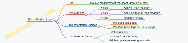
Measurement Post-Processing

Once the circuit runs, you receive bitstrings. Post-processing converts those bitstrings into expectation values like ⟨Z⟩, ⟨X⟩, or ⟨Y⟩, and then into values for multi-qubit Pauli terms.

Single-Qubit Expectation Values

For a single qubit measured in Z, map outcomes to eigenvalues:

• bit 0 → eigenvalue +1
• bit 1 → eigenvalue −1

If you measured after a basis rotation, the same mapping applies because the rotation already aligned the target axis with Z.

Example: Suppose you want ⟨X⟩ on a prepared state. You apply H, measure Z, and get counts: {“0”: 70, “1”: 30}. Then

• ⟨Z⟩ = (70 − 30) / (70 + 30) = 0.4
• Since H mapped X to Z, ⟨X⟩ = 0.4.

Multi-Qubit Pauli Terms

For a Pauli string like X⊗Y⊗Z on three qubits, you rotate each qubit according to its axis, measure all qubits in Z, and compute the product of eigenvalues for each shot.

For each shot bitstring b0 b1 b2:

• eigenvalue for qubit i is +1 if bi = 0, else −1
• the Pauli term value for that shot is the product of the three eigenvalues

Then average over shots.

Example: You measure three qubits after rotations for X⊗Y⊗Z. Suppose you have 10 shots with bitstrings:

• 000 occurs 3 times → eigenvalues (+1,+1,+1) → product +1
• 010 occurs 2 times → eigenvalues (+1,−1,+1) → product −1
• 111 occurs 5 times → eigenvalues (−1,−1,−1) → product −1

Expectation value is (3·(+1) + 2·(−1) + 5·(−1)) / 10 = (3 − 2 − 5)/10 = −0.4.

Mind Map: Post-Processing Steps

Implementation Example: Rotation Gate Selection

Below is a compact way to express basis rotation selection. The function returns the gates to apply before Z measurement.

def rotation_for_axis(axis: str):
    axis = axis.upper()
    if axis == "Z":
        return []
    if axis == "X":
        return ["H"]
    if axis == "Y":
        return ["S_DAG", "H"]
    raise ValueError(f"Unknown axis: {axis}")

A second function can compute the eigenvalue product for a measured bitstring given a Pauli string’s axes. This keeps the logic consistent: rotations affect what the bits mean, while eigenvalue mapping stays the same.

def pauli_term_value(bitstring: str):
    # bitstring like "010"
    vals = [(+1 if b == "0" else -1) for b in bitstring]
    prod = 1
    for v in vals:
        prod *= v
    return prod

Common Pitfalls and How to Avoid Them

1. Mismatched ordering: If qubit 0 corresponds to the leftmost or rightmost bit in your counts, be consistent. A wrong ordering flips signs and can quietly break optimization.
2. Forgetting that rotations change meaning: The eigenvalue mapping (+1 for 0, −1 for 1) is always for Z measurement outcomes. If you compute ⟨X⟩ or ⟨Y⟩, you must ensure rotations were applied.
3. Mixing per-qubit and per-term logic: For Pauli strings, basis choices are per qubit within the term. If you reuse a single basis across terms, you’ll measure the wrong operator.

When basis rotation and post-processing are treated as a single coherent pipeline—rotation selection, consistent bit ordering, and deterministic eigenvalue mapping—the resulting expectation values behave predictably and are easy to test with small circuits.

7.3 Expectation Value Computation from Raw Measurement Records

Expectation values turn measurement outcomes into a single number that a classical optimizer can use. The key idea is simple: expectation values are averages, and averages come from counts (or samples) plus a mapping from bitstrings to eigenvalues.

From Counts to Probabilities

Most measurement pipelines start with counts, such as { "00": 512, "01": 48, "10": 30, "11": 410 } for two qubits measured in the computational basis. Convert counts to probabilities by dividing by the total shots:

• p(bitstring) = count(bitstring) / shots

This step matters because later formulas assume probabilities, not raw counts. If you later compare results across runs with different shot counts, probability normalization keeps the comparison fair.

Choosing the Eigenvalue Mapping

For an observable like \(Z\) on one qubit, the eigenvalues are \(+1\) for measuring 0 and \(-1\) for measuring 1. For \(Z\otimes Z\) on two qubits, the eigenvalue is the product of the per-qubit eigenvalues.

A practical way to implement this is to define a function that maps each measured bitstring to an eigenvalue. For example, for \(Z\) on qubit 0 (with bitstring order matching your framework’s convention):

• if the measured bit is 0, return +1
• if the measured bit is 1, return -1

For \(Z\otimes Z\), return (+1 or -1) for each qubit and multiply them.

Computing the Expectation Value

Once you have probabilities and eigenvalues, compute:

\[ \langle O \rangle = \sum_{x} p(x),\lambda(x) \]

where \(x\) ranges over measured bitstrings and \(\lambda(x)\) is the eigenvalue for that bitstring.

Example: Single-Qubit \(Z\)

Suppose you measured one qubit with shots = 1000 and counts { "0": 620, "1": 380 }. Then:

• p(0) = 0.62, p(1) = 0.38
• λ(0) = +1, λ(1) = -1

So:

\[ \langle Z \rangle = 0.62\cdot(+1) + 0.38\cdot(-1) = 0.24 \]

This number is what you feed to the classical layer, often combined with other terms to form an energy or cost.

Example: Two-Qubit \(Z\otimes Z\)

Use counts for two qubits, shots = 1000:

• 00: 512
• 01: 48
• 10: 30
• 11: 410

Assume the bitstring is ordered as q0 q1. For each bitstring, compute \(\lambda = \lambda_{Z}(q0)\times \lambda_{Z}(q1)\):

• 00: (+1)*(+1)=+1
• 01: (+1)*(-1)=-1
• 10: (-1)*(+1)=-1
• 11: (-1)*(-1)=+1

Then:

\[ \langle Z\otimes Z \rangle = (512+410)/1000 - (48+30)/1000 = 0.844 \]

Notice how the formula groups outcomes by whether the parity of ones is even or odd.

Mind Map: Expectation Value Pipeline

Handling Bit Order and Endianness

Frameworks differ in how they present bitstrings. If your mapping assumes q0 q1 but the result is actually q1 q0, you will compute the wrong eigenvalues with no warning. A robust approach is to test mapping on a circuit that prepares a known basis state, then verify that the computed \(\langle Z \rangle\) matches the expected value.

Implementation Sketch

Below is a compact pattern for computing \(\langle Z\rangle\) from counts. It assumes bitstrings are ordered left-to-right as q0 q1 ... and that you want \(Z\) on qubit index k.

def expectation_from_counts_z(counts, shots, k, bit_order_left_to_right=True):
    exp = 0.0
    for bitstring, c in counts.items():
        p = c / shots
        bit = bitstring[k] if bit_order_left_to_right else bitstring[-1-k]
        lam = +1.0 if bit == '0' else -1.0
        exp += p * lam
    return exp

For \(Z\otimes Z\), you multiply eigenvalues for the two qubits. The rest of the pipeline stays identical: normalize, map, sum.

Practical Checks That Prevent Silent Mistakes

1. Sum of probabilities: Σ_x p(x) should be 1 (up to floating error). If not, shots or parsing is wrong.
2. Known-state sanity: Prepare |0⟩ and confirm \(\langle Z \rangle\approx +1\); prepare |1⟩ and confirm \(\langle Z \rangle\approx -1\). This catches bit-order issues.
3. Term grouping: For \(Z\otimes Z\), verify that outcomes with even parity contribute positively and odd parity negatively. If the sign pattern is flipped, the eigenvalue mapping is inverted.

Once these checks pass, expectation values become a reliable bridge from measurement records to the classical computations that follow.

7.4 Handling Multi-Qubit Observables and Efficient Term Evaluation

Multi-qubit observables are where measurement pipelines stop being “a circuit that returns bits” and start being “a system that computes numbers from structured outcomes.” The key idea is to represent an observable as a sum of terms, each term mapping to a specific measurement basis and a specific classical post-processing rule.

Term Decomposition and Measurement Grouping

A common observable form is a weighted sum of Pauli strings:

\[ O = \sum_k c_k P_k, \quad P_k \in {I, X, Y, Z}^{\otimes n} \]

Each Pauli string \(P_k\) can be measured by rotating qubits so that every non-identity factor becomes a \(Z\)-measurement. For example, \(X\otimes Z\otimes I\) requires an \(X\to Z\) basis rotation on qubit 0, no rotation on qubit 1, and nothing on qubit 2.

Efficient term evaluation comes from grouping terms that share the same measurement basis. If two Pauli strings require the same set of basis rotations, you can measure once and reuse the same sampled bitstrings to compute both terms.

Mind Map: Multi-Qubit Observable Evaluation

Converting Measurement Outcomes to Eigenvalues

For a \(Z\)-basis measurement, each qubit outcome bit \(b\in{0,1}\) corresponds to an eigenvalue \(z = +1\) if \(b=0\) and \(z=-1\) if \(b=1\). For a Pauli string term, the eigenvalue is the product of the eigenvalues for each qubit where the Pauli factor is not identity.

If you measure in a rotated basis, you still compute eigenvalues as if you measured \(Z\) after the rotation. That means the classical rule stays simple: “bit 0 means +1, bit 1 means −1,” applied to the rotated measurement results.

Example: Evaluating a Two-Qubit Observable from One Measurement Basis

Consider

\[ O = 0.5,(X\otimes X) - 1.2,(Z\otimes I) + 0.3,(I\otimes Z). \]

The terms \(X\otimes X\) and \(Z\otimes I\) do not share a basis pattern, so they belong to different groups. But \(Z\otimes I\) and \(I\otimes Z\) share the same basis pattern: both require measuring both qubits in the \(Z\) basis.

So you run:

1. One circuit for the \(X\otimes X\) group (rotate both qubits from \(X\) to \(Z\)).
2. One circuit for the \(Z\otimes I\) and \(I\otimes Z\) group (no rotations).

Now suppose the \(Z\)-basis group returns bitstrings for qubits (q0, q1). For a single shot with outcome \(b_0, b_1\):

• \(Z\otimes I\) eigenvalue is \(z_0\).
• \(I\otimes Z\) eigenvalue is \(z_1\).
• The term contribution is \(0.5\cdot (\text{from }X\otimes X\text{ group}) - 1.2,z_0 + 0.3,z_1\).

Averaging over shots gives the expectation values for those terms, then you combine them with the coefficients.

Efficient Term Evaluation via Precomputed Masks

When you have many terms, repeatedly scanning Pauli strings is slow and error-prone. A practical approach is to precompute, for each term, a mask of which qubits participate and a sign rule for the eigenvalue product.

For Pauli strings that map to \(Z\)-measurements after basis rotations, the eigenvalue product is just the product of \(z_i\) over participating qubits.

Example: Term Evaluation Skeleton

# bitstring: list[int] of 0/1 outcomes for n qubits
# z_i = +1 if bit is 0 else -1

def eigenvalue_from_mask(bitstring, mask):
    # mask: list[bool] length n, True where Pauli factor is not I
    prod = 1
    for i, use in enumerate(mask):
        if use:
            prod *= (1 if bitstring[i] == 0 else -1)
    return prod

# For a term: expectation is average over shots of eigenvalue_from_mask

This keeps the classical logic consistent across terms within a basis group. The only thing that changes between terms is the mask.

Handling Y Terms Without Complicating the Post-Processing

A \(Y\) factor is handled by the quantum basis rotation, not by changing the classical eigenvalue rule. After the appropriate rotation, the measurement is still treated as \(Z\) outcomes, so the same bit-to-±1 mapping applies.

The practical implication is that your post-processing should not branch on whether a term contains \(X\), \(Y\), or \(Z\). It should branch only on which qubits are non-identity for that term, because the basis rotation has already done the heavy lifting.

Validation Checks That Catch Real Bugs

Two checks prevent most “it runs but the numbers are wrong” issues:

1. Basis Pattern Consistency: every term in a basis group must require the same rotation pattern. A single mismatched term can silently corrupt the expectation.
2. Mask Correctness: identity factors must be excluded from the eigenvalue product. If you accidentally include an identity qubit, the term becomes a different observable.

A quick spot-check uses a known state where the expected value is easy to compute, such as a computational basis state for \(Z\)-only terms. If \(Z\)-only terms fail, the issue is almost certainly in bit ordering, mask construction, or eigenvalue mapping.

7.5 Validating Measurement Pipelines with Known Reference States

A measurement pipeline is only as trustworthy as its ability to reproduce outcomes you already understand. Known reference states give you that anchor: you can check that your circuit preparation, basis rotations, measurement extraction, and expectation-value computation all agree with a target you can compute exactly.

What “Known Reference” Means in Practice

A reference state should satisfy two properties. First, you can prepare it deterministically in your chosen framework. Second, you know what the measurement statistics should look like for the observables you plan to test.

For example, the computational basis states

Bell states like (|00⟩+|11⟩)/√2 give predictable correlations for ZZ and XX.

If your pipeline is correct, the measured expectation values should match the known targets within your statistical uncertainty.

A Minimal Validation Checklist

Use the same sequence every time so failures are easy to localize.

1. State preparation check: verify that the prepared state matches the intended one under a simple measurement.
2. Basis rotation check: confirm that your basis-change logic maps the intended observable to a Z measurement.
3. Extraction check: ensure bit ordering and endianness are consistent between circuit output and post-processing.
4. Expectation computation check: validate the mapping from counts to expectation values for single- and multi-qubit observables.
5. Metadata check: confirm that shot counts and run identifiers are carried through without accidental mixing.

Mind Map: Measurement Validation Flow

Example: Single-Qubit Z and X with Deterministic Targets

Suppose your pipeline takes a circuit that prepares a state, applies a basis rotation for an observable, measures, and returns an expectation value.

• Reference state |0⟩: for Z, the expectation value should be +1.
• Reference state |1⟩: for Z, the expectation value should be −1.
• Reference state |+⟩: for X, the expectation value should be +1.
• Reference state |−⟩: for X, the expectation value should be −1.

A common bug is that basis rotation is correct but bit ordering is flipped. You can catch that quickly by testing both |0⟩ and |1⟩. If your Z expectation for |0⟩ is near +1 but for |1⟩ is not near −1, the issue is likely in extraction or eigenvalue mapping, not in state preparation.

Example: Two-Qubit Correlations with Bell States

Take the Bell state

Known targets:

• ⟨ZZ⟩ = +1
• ⟨XX⟩ = +1
• ⟨YY⟩ = +1 (if you implement Y-basis rotation correctly)

Validation strategy:

1. Prepare |Φ+⟩.
2. For ZZ, measure both qubits directly in the computational basis and compute parity.
3. For XX, apply the correct basis rotation to map X to Z before measuring.

If ⟨ZZ⟩ is correct but ⟨XX⟩ is wrong, the failure is almost certainly in the basis rotation logic for X. If both are wrong, check state preparation and bit ordering first.

Example: A Concrete Expectation-Value Computation Test

For a single-qubit Z observable, eigenvalues are +1 for measuring bit 0 and −1 for measuring bit 1. Given counts like {'0': c0, '1': c1}, the expectation is:

• p0 = c0 / (c0 + c1)
• p1 = c1 / (c0 + c1)
• ⟨Z⟩ = (+1)·p0 + (−1)·p1

For two-qubit ZZ, eigenvalue is +1 when bits match (00 or 11) and −1 when they differ (01 or 10). This parity rule is a great place to test bit ordering: if you swap qubit indices, the parity rule still holds, but the mapping from measured string positions to qubits changes. Your pipeline should be consistent about which character in the bitstring corresponds to which qubit.

Comparison with Statistical Error Bars

Even with perfect logic, finite shots produce variation. Use a simple tolerance based on the binomial variance of the measurement outcomes. For deterministic targets like ±1, the observed mean should concentrate near the target as shots increase.

When you see a consistent offset (not just noise), treat it as a systematic issue. The fastest way to localize is to rerun the same reference state with a simpler observable. If Z works and X fails, you’ve narrowed the problem to basis rotation and observable mapping.

What to Record During Validation

Store, for each test:

• reference state identifier
• observable requested
• basis rotation applied
• raw counts or probabilities
• computed expectation value
• target value
• tolerance used

This turns debugging from “why is it off?” into “which step disagrees with the known target?”

8.1 Building Variational Circuits with Shared Parameter Schemas

A variational circuit is only as reusable as its parameter story. “Shared parameter schemas” means you define one consistent set of parameter names, shapes, and binding rules that both frameworks can consume without rewriting your algorithm logic.

What a Shared Parameter Schema Means

A schema specifies:

• Parameter identity: stable names like theta[0], theta[1], not framework-specific objects.
• Parameter ordering: a deterministic mapping from index to circuit location.
• Parameter grouping: which parameters belong to which layer, block, or gate family.
• Binding interface: a function that takes a numeric vector and produces the bindings required by Qiskit and Cirq.

If you keep these four items fixed, you can swap circuit templates, simulators, and even frameworks while preserving the meaning of each parameter.

Mind Map: Parameter Schema Design

Mind Map: Shared Parameter Schema

A Concrete Schema: Layered Ry-Rz Ansatz

Consider an ansatz with L layers on n qubits. Each layer applies, for each qubit q, an Ry rotation followed by an Rz rotation. That yields 2 * L * n parameters.

Define the schema index as:

• theta[ idx(layer, q, kind) ]
• where kind = 0 for Ry, kind = 1 for Rz
• and idx(layer, q, kind) = (layer * n + q) * 2 + kind

This gives you a single parameter vector layout that is easy to generate, slice, and debug.

Example: Parameter Vector Layout and Slicing

Let n=2, L=2. Then there are 2*2*2 = 8 parameters: theta[0]..theta[7].

• Layer 0
  • q0: Ry = theta[0], Rz = theta[1]
  • q1: Ry = theta[2], Rz = theta[3]
• Layer 1
  • q0: Ry = theta[4], Rz = theta[5]
  • q1: Ry = theta[6], Rz = theta[7]

When an optimizer proposes a vector, you can immediately interpret which layer and qubit it is affecting.

Example: Qiskit Template with Schema-First Parameters

from qiskit.circuit import QuantumCircuit, Parameter

def build_ansatz_qiskit(n, L):
    qc = QuantumCircuit(n)
    theta = [Parameter(f"theta[{i}]") for i in range(2*L*n)]

    def idx(layer, q, kind):
        return (layer*n + q)*2 + kind

    for layer in range(L):
        for q in range(n):
            qc.ry(theta[idx(layer, q, 0)], q)
            qc.rz(theta[idx(layer, q, 1)], q)
    return qc, theta

This template is built once. Later, you bind a numeric vector by mapping each Parameter to its corresponding value.

Example: Cirq Template with the Same Schema

import cirq

def build_ansatz_cirq(n, L):
    qubits = [cirq.LineQubit(i) for i in range(n)]
    theta = [cirq.Symbol(f"theta[{i}]") for i in range(2*L*n)]

    def idx(layer, q, kind):
        return (layer*n + q)*2 + kind

    circuit = cirq.Circuit()
    for layer in range(L):
        for q in range(n):
            circuit.append(cirq.ry(theta[idx(layer, q, 0)])(qubits[q]))
            circuit.append(cirq.rz(theta[idx(layer, q, 1)])(qubits[q]))
    return circuit, theta

The key is that both templates use the same theta[i] naming scheme and the same indexing function.

Binding Interface and Validation

A practical best practice is to centralize binding in one place. Even if you bind differently per framework, you should validate the vector length and ensure every expected parameter is present.

Mind the failure modes:

• Off-by-one indexing: the circuit still runs, but the optimizer is optimizing the wrong gates.
• Unbound parameters: some frameworks will error; others may produce confusing results.
• Extra parameters: you think you’re optimizing 2*L*n, but the circuit contains more.

Mind Map: Binding and Checks

A Small Test Vector That Catches Index Bugs

Use a vector where only one entry is nonzero, like theta[k]=0.1 and all others 0.0. Then run the circuit and confirm that only the intended Ry or Rz gate changes. This is boring in the best way: it turns indexing mistakes into immediate, observable behavior.

Shared parameter schemas make your variational code easier to reason about because the optimizer’s vector and the circuit’s gates stay in lockstep, even when you switch frameworks or refactor templates.

8.2 Gradient Estimation Using Finite Differences in Practice

Finite differences estimate how an objective changes when you nudge parameters. In hybrid quantum-classical code, that means: pick a parameter vector \(\theta\), evaluate the objective at \(\theta+\epsilon e_i\) and \(\theta-\epsilon e_i\), then approximate the derivative with respect to \(\theta_i\). The method is simple, but the details decide whether it’s stable or noisy.

Core Idea and Two Common Formulas

For a scalar objective \(f(\theta)\) and parameter index \(i\):

• Forward difference: \(\partial_i f(\theta) \approx \frac{f(\theta+\epsilon e_i)-f(\theta)}{\epsilon}\)
• Central difference: \(\partial_i f(\theta) \approx \frac{f(\theta+\epsilon e_i)-f(\theta-\epsilon e_i)}{2\epsilon}\)

Central differences usually behave better because the leading error term cancels. The tradeoff is that you need twice as many objective evaluations per parameter.

Choosing \(\epsilon\) Without Guessing Blindly

Too large \(\epsilon\) biases the derivative because you’re measuring a slope over a wide interval. Too small \(\epsilon\) amplifies statistical noise from finite shots and can make the gradient look like it’s doing interpretive dance.

A practical approach is to treat \(\epsilon\) as a knob and check gradient consistency:

1. Pick a baseline \(\epsilon_0\).
2. Compute gradients with \(\epsilon_0\) and \(\epsilon_0/2\) using the same shot budget.
3. If the direction flips wildly, increase \(\epsilon\) or increase shots.

This doesn’t guarantee perfection, but it prevents the most common failure mode: “the optimizer is optimizing noise.”

Mind Map for Finite-Difference Gradients

Example: Estimating Energy Gradient from Measured Expectation

Assume your objective is an energy estimate from an observable \(H\):

\[ f(\theta)=\langle H \rangle_{\theta} \]

In practice, \(\langle H \rangle\) is computed from measurement outcomes. Suppose \(H\) is a weighted sum of Pauli terms, and your code already returns \(f(\theta)\) as a float using a fixed shot count.

Let \(\theta=[\theta_0,\theta_1]\). Central differences require four objective calls:

• \(f(\theta_0+\epsilon,\theta_1)\)
• \(f(\theta_0-\epsilon,\theta_1)\)
• \(f(\theta_0,\theta_1+\epsilon)\)
• \(f(\theta_0,\theta_1-\epsilon)\)

Then:

\[ \partial_{\theta_0} f \approx \frac{f(\theta_0+\epsilon,\theta_1)-f(\theta_0-\epsilon,\theta_1)}{2\epsilon} \]

\[ \partial_{\theta_1} f \approx \frac{f(\theta_0,\theta_1+\epsilon)-f(\theta_0,\theta_1-\epsilon)}{2\epsilon} \]

A subtle but important detail: keep the circuit structure identical across evaluations. Only bind parameter values; do not rebuild the circuit in a way that changes measurement ordering or transpilation randomness.

Example Code Skeleton for Central Differences

The snippet below assumes you have a callable objective(theta) that returns a scalar using a fixed shot budget.

import numpy as np

def finite_diff_grad(objective, theta, eps):
    theta = np.asarray(theta, dtype=float)
    grad = np.zeros_like(theta)

    for i in range(len(theta)):
        e = np.zeros_like(theta)
        e[i] = 1.0
        theta_plus = theta + eps * e
        theta_minus = theta - eps * e
        f_plus = objective(theta_plus)
        f_minus = objective(theta_minus)
        grad[i] = (f_plus - f_minus) / (2.0 * eps)

    return grad

If your objective returns both value and an estimated standard error, you can propagate uncertainty into the gradient magnitude. Even a rough estimate helps you decide whether to increase shots or adjust \(\epsilon\).

Reliability Checks That Pay Off

1. Gradient direction stability: compute gradients at \(\epsilon\) and \(\epsilon/2\) and compare cosine similarity.
2. Shot budget consistency: use the same shot count for \(f(\theta^+)\) and \(f(\theta^- )\) so the difference isn’t dominated by unequal variance.
3. Parameter scaling: if parameters have very different units or typical magnitudes, consider scaling \(\epsilon\) per parameter so the perturbation is meaningful in each coordinate.

Mind Map for Reliability and Debugging

Finite differences are a dependable baseline when you want correctness first and differentiation tricks second. With careful \(\epsilon\) selection, consistent execution settings, and a couple of sanity checks, the gradients become usable rather than merely computed.

8.3 Implementing Parameter-Shift Style Workflows With Software Controls

Parameter-shift style workflows estimate gradients by running the same circuit multiple times with controlled parameter offsets, then combining the results with a fixed formula. The “software controls” part is what keeps the workflow correct when you have batching, shot noise, caching, and multiple parameters.

Mind Map: Parameter-Shift Workflow Controls

Choosing a Shift Rule That Matches Your Circuit

A common parameter-shift rule applies when the gate generating the parameter has a simple spectrum, often leading to a two-run estimate:

• Run at θ + s
• Run at θ − s
• Combine as (f(θ + s) − f(θ − s)) / (2 sin s)

Software control should encode the shift rule explicitly rather than scattering “magic numbers” across the code. A practical approach is to represent each parameter as a small record: its shift value, its coefficient, and which circuit parameters it affects.

Example: Two-Run Gradient for One Parameter

Assume your circuit returns an expectation value f(θ) = ⟨O⟩. You want df/dθ.

import math

def parameter_shift_gradient(expect_fn, theta, shift):
    f_plus = expect_fn(theta + shift)
    f_minus = expect_fn(theta - shift)
    denom = 2.0 * math.sin(shift)
    return (f_plus - f_minus) / denom

The key control is expect_fn: it should take a scalar θ, bind it into the circuit, run the measurement, and return a single expectation value. If you later switch from simulator to hardware, you should not touch the gradient formula.

Example: Multi-Parameter Run Plan with Deduplication

When you have parameters θ₀…θₙ₋₁, a naive implementation runs 2n circuits per gradient step. That’s fine for small n, but it becomes wasteful if your parameter binding produces identical circuits due to shared parameters or repeated values.

A control layer can generate a run plan keyed by a normalized binding dictionary.

from dataclasses import dataclass

@dataclass(frozen=True)
class ShiftSpec:
    name: str
    shift: float
    coeff: float

def make_run_plan(base_bind, specs):
    plan = []
    for spec in specs:
        for sign in (+1, -1):
            bind = dict(base_bind)
            bind[spec.name] = base_bind[spec.name] + sign * spec.shift
            plan.append((spec, sign, bind))
    return plan

Then you can deduplicate by hashing bind into a canonical tuple order. The gradient assembly uses only the results for each parameter’s plus and minus bindings.

Example: Shot-Aware Expectation Evaluation

Parameter-shift estimates are sensitive to shot noise because you subtract two noisy estimates. A simple control policy is to keep shot counts consistent across plus and minus runs for each parameter, and optionally increase shots when the difference is small.

def expectation_from_counts(counts, observable_map):
    # observable_map maps bitstrings to eigenvalues (+1/-1 etc.)
    total = sum(counts.values())
    exp = 0.0
    for bitstring, c in counts.items():
        exp += (c / total) * observable_map[bitstring]
    return exp

Your execution function should return both the expectation and the effective shot count so you can track whether a gradient component is dominated by sampling error.

Result Validation That Prevents Silent Bugs

Two failure modes show up often: (1) binding the wrong parameter name, and (2) mixing measurement conventions between runs. Software controls should include checks that are cheap compared to running circuits.

• Verify that every shift binding changes only the intended parameter.
• Verify that the measurement post-processing uses the same bit ordering for all runs.
• Verify that expectation values are finite numbers.

A practical pattern is to attach a small “run signature” to each job: parameter name, sign, shift, and the bound value. When results return, you match them back to the signature.

Assembling Gradients with Coefficients

Some shift rules include coefficients beyond the basic two-run formula. Your gradient assembler should accept a list of ShiftSpec objects and compute:

• f_plus and f_minus per parameter
• gradient = coeff * (f_plus − f_minus)

This keeps the formula consistent even if you later support different gate types or different shift rules.

Mind Map: Software Controls for Correctness

Putting It Together in a Hybrid Optimizer Loop

In a hybrid loop, you typically call a classical optimizer that asks for gradients at a parameter vector. The software control should treat “gradient evaluation” as a single unit: generate run plan, execute all required measurements, validate results, then return a gradient vector. That boundary prevents partial failures from leaking into the optimizer state.

A good rule of thumb: if you can’t explain how a single gradient component was computed from specific plus/minus bindings and specific measurement outputs, you don’t yet have enough controls.

8.4 Integrating Gradients into Classical Optimizers Safely

A variational loop usually looks simple: build a parameterized circuit, run it to estimate an objective, compute gradients, and let a classical optimizer update parameters. The “safe” part is making sure gradients match the objective you actually estimated, and that the optimizer never receives values that are inconsistent, mis-scaled, or silently wrong.

Gradient Contracts That Prevent Silent Bugs

Define a contract for your gradient function so it always returns gradients with the same parameter ordering, shape, and scaling as the objective value.

• Parameter ordering: Use a single source of truth for parameter names or indices. If you bind parameters in a different order than you compute gradients, the optimizer will dutifully optimize the wrong directions.
• Shape consistency: Return a flat vector of length n_params (or a 2D array if your optimizer expects it). Avoid returning nested lists that “look right” but get broadcast incorrectly.
• Scaling consistency: If your objective is an expectation value, keep gradients in the same units. If you average over terms or normalize by shot counts, apply the same normalization to gradients.
• Noise awareness: With finite shots, gradients are noisy. Safety means you either (a) compute gradients in a way that matches the shot model you used for the objective, or (b) explicitly treat gradients as estimates and adjust stopping and step sizes accordingly.

Choosing a Gradient Strategy That Matches Your Estimator

There are two common patterns.

1. Finite differences: Evaluate the objective at θ + ε and θ - ε for each parameter. This is easy to reason about but expensive and sensitive to shot noise.
2. Parameter-shift style rules: For certain gate structures, you can compute gradients from a small set of shifted circuit evaluations. This is often more stable than naive finite differences, but only applies when the circuit supports the rule.

Safety rule: your gradient method must call the same measurement pipeline as the objective estimator. If the objective uses post-processing (basis rotations, term grouping, or observable mapping), gradients must use the same post-processing.

Mind Map: Safe Gradient Integration

Example: Finite Differences with Shot-Matched Objective

Assume your objective function returns an expectation value estimated from samples. A safe finite-difference gradient uses the same shot count and the same objective code path.

import numpy as np

def objective(theta, shots):
    # Returns a scalar expectation value using the same pipeline
    # as the gradient will rely on.
    return run_quantum_objective(theta, shots=shots)

def finite_diff_grad(theta, shots, eps=1e-3):
    theta = np.asarray(theta, dtype=float)
    n = theta.size
    grad = np.zeros(n, dtype=float)
    base = objective(theta, shots=shots)
    for i in range(n):
        d = np.zeros(n)
        d[i] = eps
        f_plus = objective(theta + d, shots=shots)
        f_minus = objective(theta - d, shots=shots)
        grad[i] = (f_plus - f_minus) / (2.0 * eps)
    return grad

Safety notes embedded in the code logic: it uses central differences, it calls objective for both shifted points, and it keeps shots identical across evaluations.

Example: Guardrails for Optimizer Inputs

Optimizers often assume gradients are finite numbers. Add checks before returning gradients.

def safe_grad(theta, shots, grad_fn):
    g = grad_fn(theta, shots=shots)
    g = np.asarray(g, dtype=float)
    if not np.all(np.isfinite(g)):
        raise ValueError("Non-finite gradient encountered")
    # Optional: clip to reduce the impact of shot noise spikes.
    max_norm = 10.0
    norm = np.linalg.norm(g)
    if norm > max_norm:
        g = g * (max_norm / norm)
    return g

Clipping is not a substitute for correct gradients, but it prevents a single noisy batch from sending parameters into a region where the objective estimator becomes unstable.

Example: Spot-Checking Gradients in Deterministic Mode

Before trusting gradients under shot noise, verify them in a deterministic setting (simulator with fixed sampling behavior or analytic evaluation). A practical check compares your gradient method against finite differences using a small eps.

def gradient_sanity_check(theta, shots, eps=1e-4):
    g_shift = safe_grad(theta, shots, grad_fn=parameter_shift_grad)
    g_fd = finite_diff_grad(theta, shots=shots, eps=eps)
    rel_err = np.linalg.norm(g_shift - g_fd) / (np.linalg.norm(g_fd) + 1e-12)
    return rel_err

If the relative error is large in deterministic mode, fix the gradient computation or the parameter binding order before running a noisy hybrid loop.

Practical Integration Checklist

• Use one parameter ordering everywhere: circuit binding, objective evaluation, and gradient computation.
• Ensure gradients call the same measurement and post-processing as the objective.
• Keep shot counts consistent across objective and gradient evaluations.
• Validate gradients in deterministic mode with a finite-difference spot-check.
• Reject non-finite gradients and consider clipping to reduce shot-noise spikes.
• Log parameter vectors, objective values, and gradient norms per iteration for traceability.

When these pieces line up, the optimizer becomes a reliable consumer of gradient information rather than a generator of confusion.

8.5 Debugging Convergence Issues with Circuit-Level Diagnostics

Convergence problems in variational or hybrid loops usually come from one of three places: the circuit is not expressing what you think it is, the measurement pipeline is producing numbers with the wrong meaning, or the optimizer is receiving gradients or objective values that are internally inconsistent. Circuit-level diagnostics help you separate those causes quickly by checking invariants before you blame the optimizer.

What to Check First

Start with invariants that should hold regardless of the backend.

1. Parameter binding is correct. If you use parameterized circuits, confirm that every symbolic parameter is bound to a numeric value before execution. A common failure mode is a parameter left unbound, which can silently default or error depending on the framework.
2. The circuit you think you built is the circuit you executed. Transpilation and compilation steps can reorder operations, insert swaps, and change gate sets. You want to inspect the compiled circuit that actually ran.
3. Measurement semantics match the observable. If you compute an expectation value, verify that the basis rotations and bit ordering correspond to the observable definition.
4. The objective is computed from the same shots and the same mapping. If you batch terms or reuse results, ensure you are not mixing counts from different runs or different qubit layouts.

Circuit-Level Diagnostics Mind Map

Example: Detecting Misbound Parameters

Suppose your variational ansatz uses parameters theta_0, theta_1, and theta_2, but your binding dictionary accidentally uses theta1 (missing underscore). The circuit still runs, yet the effective parameters are wrong, and the optimizer can’t find a meaningful direction.

Use a diagnostic that asserts every parameter in the circuit has a bound value.

# Example: parameter binding validation
# Works conceptually for both frameworks with minor API differences.

def assert_all_params_bound(circuit, param_values):
    # circuit.parameters is a set of symbolic parameters
    missing = [p for p in circuit.parameters if p not in param_values]
    if missing:
        raise ValueError(f"Unbound parameters: {missing}")

# Usage: before execution
# assert_all_params_bound(ansatz_circuit, {theta_0: 0.1, theta_1: 0.2, theta_2: 0.3})

If you see missing parameters, fix the naming and rerun with a tiny number of shots. You should observe the loss change when you perturb parameters.

Example: Comparing Pre- and Post-Transpile Circuits

Even if your ansatz is correct, transpilation can change gate structure. For convergence debugging, you don’t need to understand every compiler decision; you need to confirm that the compiled circuit still implements the same logical operations on the intended qubits.

A practical approach is to compare:

• The qubit mapping after compilation.
• The presence of basis rotation gates used for measurement.
• The final measurement instruction locations.

If your compiled circuit measures different physical qubits than your post-processing assumes, your expectation values will be wrong even though the code runs.

Example: Verifying Measurement Basis and Bit Ordering

Imagine you want an expectation value of Z on qubit 0. If your post-processing interprets bitstrings with the wrong endianness, you effectively compute Z on a different qubit. The optimizer then chases a moving target.

A simple diagnostic is to run a circuit that prepares a known state and measure it.

# Example: bit-order sanity check
# Prepare |0> and |1> on a single qubit and ensure counts match.

def sanity_counts(simulator_run_fn):
    # Run two circuits: one that prepares |0>, one that prepares |1>
    counts0 = simulator_run_fn(prep_zero=True)
    counts1 = simulator_run_fn(prep_zero=False)

    # Expect most shots in the all-zeros bitstring for |0>
    # and in the bitstring with the target bit set for |1>.
    return counts0, counts1

If the “|1>” case shows the excitation on the opposite bit position, fix your bit ordering in the expectation computation.

Example: Minimal Circuit Reduction

When convergence is broken, reduce the problem until you can reason about it.

1. Keep only one parameterized gate layer.
2. Use a single observable term.
3. Use a small shot count.
4. Sweep one parameter across a grid and plot the objective.

If the objective is constant across the sweep, the circuit likely isn’t sensitive to that parameter (wrong binding, gate canceled by compilation, or measurement not connected to the parameterized part). If it changes but the optimizer still fails, the issue is more likely in gradient estimation or objective aggregation.

Diagnostic Checklist You Can Automate

• Assert all parameters are bound.
• Log the compiled circuit and qubit mapping.
• Assert measurement instructions exist where your post-processing expects.
• Validate bit ordering with a known-state test.
• Compute expectation values from a single term using fresh results, not cached mixed batches.

Convergence debugging becomes much less mysterious when you treat the circuit as a contract: parameters must flow into the compiled operations, measurements must map to the observable definition, and the objective must be computed from consistent raw data.

9.1 Aligning Circuit Semantics Across Frameworks for Meaningful Comparisons

When you compare Qiskit and Cirq results, you’re really comparing semantics: what a circuit means, not just what it looks like. The tricky part is that both frameworks can express similar ideas while choosing different defaults for qubit ordering, measurement mapping, and parameter handling. Meaningful comparisons start by writing down a shared contract for those choices.

Semantic Contract Checklist

1. Qubit indexing and bit order

   • Decide whether “qubit 0” is the least-significant bit (LSB) or most-significant bit (MSB) in your classical readout.
   • Decide how multi-qubit measurement strings are ordered in each framework’s output.

2. Measurement convention

   • Confirm whether measurements are taken in the computational basis only, or whether basis rotations are explicitly inserted.
   • Ensure post-processing uses the same convention for converting raw outcomes into expectation values.

3. Gate meaning and decomposition

   • Compare at the level of unitary intent, not at the level of gate names.
   • If you transpile in Qiskit, record the final gate set and connectivity assumptions so Cirq can be compared against the same effective circuit.

4. Parameter binding rules

   • Use the same parameter values and the same parameter-to-qubit mapping.
   • Avoid mixing symbolic parameters with framework-specific binding behavior unless you normalize them first.

5. Noise and sampling assumptions

   • For fair comparisons, either both sides are noiseless or both sides use equivalent noise models.
   • Match shot counts and sampling strategy, then compare statistical summaries with the same definitions.

Mind Map: Semantic Alignment Targets

Example: Same Circuit, Different Readout Strings

Consider a two-qubit circuit that prepares a Bell state and measures both qubits. If one framework reports outcomes as q1q0 while the other reports q0q1, you’ll think the circuits disagree even when they don’t.

Goal: normalize measurement strings into a shared ordering before comparing.

• Choose a canonical ordering: say, classical bitstring is q0 q1.
• If Qiskit returns strings in q1 q0, reverse them.
• If Cirq returns in q0 q1, keep them.

A practical approach is to write a small adapter that converts each framework’s outcome keys into the canonical ordering, then compare distributions.

Example: Canonical Outcome Adapter Logic

def canonicalize_outcome_key(key: str, source_order: str, canonical_order: str) -> str:
    # source_order and canonical_order are like "q0q1" or "q1q0"
    pos = {q: i for i, q in enumerate(source_order)}
    canon_pos = {q: i for i, q in enumerate(canonical_order)}
    bits = ['0'] * len(canonical_order)
    for q in canonical_order:
        bits[canon_pos[q]] = key[pos[q]]
    return ''.join(bits)

This adapter is boring on purpose: it makes the comparison about probabilities, not about string formatting.

Example: Effective Circuit Comparison After Transpilation

Qiskit often transpiles circuits to match backend constraints, which can change the gate sequence while preserving the intended unitary (up to numerical tolerance). If you compare that transpiled circuit to a Cirq circuit that still uses the original high-level gates, you may see differences.

To align semantics:

1. Compare the effective circuit: use the transpiled Qiskit circuit as the reference.
2. Re-express the same effective operations in Cirq: either by constructing Cirq operations that match the transpiled gate list, or by ensuring both sides use the same decomposition rules.
3. Verify with a noiseless statevector check: for small circuits, compare statevectors or exact probabilities after alignment.

Example: Parameter Binding Consistency

Suppose you have a parameterized rotation gate on a specific qubit. In Qiskit, parameters are bound by name; in Cirq, you may bind by symbol resolution. Misalignment happens when the same symbol name exists but is bound to the wrong value or applied to the wrong wire.

A reliable pattern is:

• Create a single dictionary of parameter values.
• Apply it explicitly to both frameworks.
• Assert that the resulting numeric circuit has the same parameter values on the same qubits.

Putting It Together: A Comparison Workflow

1. Define canonical qubit order and canonical bitstring format.
2. Build circuits with explicit measurement operations and explicit basis rotations.
3. Normalize measurement outputs into canonical bitstrings.
4. Ensure both sides use the same effective gate set (or verify equivalence noiselessly).
5. Compare probability distributions and derived expectation values using identical post-processing.

If you do these steps, “meaningful comparisons” becomes a mechanical process: you’re checking whether the same intended quantum operation produces the same measured statistics, not whether two frameworks chose the same defaults.

9.2 Converting Gate Sets and Handling Differences in Defaults

When you move circuits between Qiskit and Cirq, the biggest surprises usually come from “defaults,” not from the gates themselves. A conversion that looks correct at the gate level can still change behavior because of implicit assumptions about qubit ordering, basis conventions, parameter types, and how measurement is represented.

What “Gate Set Conversion” Really Means

Gate set conversion is not just mapping names like rx to XPowGate. It also includes:

• Unit conventions: Qiskit’s rx(θ) uses radians, while Cirq’s exponent-based gates often use a fraction of a full turn.
• Direction and phase conventions: Some gates are equivalent up to global phase, which is fine for probabilities but not for state comparisons.
• Decomposition targets: Qiskit may transpile into a backend’s basis, while Cirq typically keeps a higher-level moment structure unless you explicitly decompose.

A practical rule: treat conversion as a two-step process—first map semantics, then verify with a small set of reference inputs.

Default Differences That Commonly Break Equivalence

1. Qubit indexing and bit ordering

   • Qiskit circuits often label qubits in a register, and classical bits may be ordered differently from measurement results.
   • Cirq measurement keys produce results keyed by the moment’s measurement operations.

2. Measurement representation

   • Qiskit commonly returns counts or quasi-distributions from measured classical bits.
   • Cirq returns measurement arrays per key, and you decide how to interpret them.

3. Implicit basis rotations

   • Some measurement workflows add basis rotations automatically in one framework and not the other.
   • If you convert only the circuit and not the measurement pipeline, expectation values can shift.

4. Parameter binding behavior

   • Qiskit parameters are symbolic until you bind them; Cirq uses parameter resolvers tied to symbols.
   • If you convert a parameterized circuit without preserving symbol identity, you can bind the wrong values.

Gate Mapping Patterns with Concrete Examples

Example: Mapping Rotation Gates

In Qiskit, a typical rotation is RX(θ). In Cirq, cirq.rx(θ) exists, but exponent-based forms like XPowGate(exponent=t) use a different parameterization. If you use XPowGate(exponent=t), then the rotation angle is π * t.

Example mapping logic:

• Qiskit RX(θ) ↔ Cirq XPowGate(exponent=θ/π)
• Qiskit RZ(λ) ↔ Cirq ZPowGate(exponent=λ/π)

If you instead use Cirq’s direct helpers like cirq.rx(θ), you avoid the exponent conversion and reduce mistakes.

Example: Mapping Controlled Operations

Qiskit’s CX is a controlled-NOT. Cirq’s equivalent is CNOT(control, target).

However, controlled gates can differ when you convert more general controlled rotations. Qiskit may represent them as a single gate that later decomposes, while Cirq might require explicit decomposition into elementary operations. If you compare only the high-level circuit, you can miss a mismatch introduced during decomposition.

A Conversion Workflow That Stays Honest

1. Normalize both circuits to a shared intermediate form

   • Choose a target set like {H, X, Z, S, T, CX, RZ} or a small universal set.
   • Convert both frameworks into that set using explicit decomposition.

2. Make qubit order explicit

   • Define a mapping qiskit_index -> cirq_qubit and keep it consistent for every conversion.

3. Separate circuit conversion from measurement conversion

   • Convert the unitary part first.
   • Then rebuild measurement logic with explicit basis rotations and explicit bit interpretation.

4. Verify with reference states

   • Test a handful of basis states like |00⟩, |01⟩, |10⟩, |11⟩ for two-qubit circuits.
   • Compare measurement probabilities, not just gate lists.

Mind Map: Defaults That Affect Conversion

Example: A Minimal Cross-Framework Equivalence Check

Suppose you have a two-qubit circuit with H on qubit 0 and CX from qubit 0 to qubit 1, followed by measurement.

• Convert the unitary portion first.
• Then apply the same measurement interpretation on both sides: same qubit-to-bit mapping, same basis (no hidden rotations).
• Finally, run on basis states and confirm that the output probabilities match.

If the probabilities match but the raw bitstrings differ, the issue is likely bit ordering, not the gate conversion.

Practical Guidance for Handling Defaults Without Guesswork

• Prefer Cirq’s direct rotation helpers when possible to avoid exponent math.
• When converting, always carry a qubit mapping object and use it for both circuit and measurement.
• Treat decomposition as an explicit step: if one framework decomposes automatically and the other doesn’t, you will compare different circuits.
• Validate with probability checks on small inputs before scaling up.

9.3 Normalizing Measurement Conventions and Bit Ordering

When you mix Qiskit and Cirq, the most common “it runs but the numbers look wrong” problem is bit ordering. Both frameworks can measure the same physical qubits, yet produce different classical bit strings depending on how they map qubit indices to result bits. Normalization is the discipline of converting every framework’s raw measurement output into one shared, explicit convention.

Define One Canonical Convention

Pick a single rule and stick to it across the whole hybrid program. A practical choice is:

• Qubit order: qubit index increasing from left to right in your logical bit vector.
• Bit vector representation: b[0] corresponds to qubit 0, b[1] to qubit 1, etc.
• Measurement output: a list or array of bits in that order, not a framework-specific string.

Then treat framework outputs as “wire formats” that must be converted into this canonical representation.

Understand How Each Framework Emits Bits

Qiskit typically returns counts or bitstrings where the leftmost character corresponds to the highest-index classical bit in the returned string. Cirq returns measurement arrays whose axes correspond to qubits and repetitions, and the mapping depends on how you pass qubits to the measurement operation.

The key is not memorizing which side is reversed, but verifying the mapping with a tiny circuit that you can reason about without simulation.

Use a Two-Qubit Sanity Circuit

Create a circuit that forces a known measurement pattern. For example, prepare qubit 0 in |1⟩ and qubit 1 in |0⟩, then measure both.

Example:

# Qiskit-style pseudocode
# Prepare: q0=1, q1=0
# Measure both qubits into a single classical register
# Then compare the produced bitstring to the expected [b0,b1]=[1,0]

Run the same logical preparation in Cirq and record how each framework orders the bits in its output. You are not testing physics; you are testing the software’s convention.

Convert Raw Outputs into Canonical Bit Vectors

Once you know the mapping, implement a small normalization function that:

1. Takes the raw measurement output (bitstring or measurement array).
2. Produces b[0..n-1] where b[i] is the measurement of qubit i.
3. Returns the same type every time (e.g., a Python list of ints).

Example:

def normalize_bitstring(bitstring, n, left_to_right_is_highest_index):
    # bitstring length should be n
    if left_to_right_is_highest_index:
        # e.g., Qiskit-like: leftmost char corresponds to highest classical bit
        # Map to canonical b[i] where i increases with qubit index.
        return [int(bitstring[n-1-i]) for i in range(n)]
    else:
        return [int(bitstring[i]) for i in range(n)]

If you later change register layout or measurement grouping, you update only the mapping flag (or the mapping logic), not every downstream algorithm.

Normalize Across Repetitions and Batches

Hybrid loops often run many shots. Ensure your normalization preserves the repetition axis.

• For counts/bitstrings, expand each bitstring into a canonical bit vector and keep the count.
• For measurement arrays, reorder axes or indices so that the qubit axis matches qubit index order.

A good invariant is: for every repetition r, the normalized vector b_r must satisfy b_r[i] == measured_value_of_qubit_i_in_that_repetition.

Mind Map: Measurement Conventions and Bit Ordering

Mind Map: Normalizing Measurement Conventions

Example: Cross-Framework Consistency Check

After normalization, you should be able to compare results from both frameworks using the same post-processing.

Example workflow:

• Run the sanity circuit in Qiskit and Cirq with the same number of shots.
• Normalize every observed outcome into canonical bit vectors.
• Compute a simple statistic like the fraction of shots where b[0]=1 and b[1]=0.

If the fractions match (within sampling noise), your bit ordering is consistent. If not, the normalization mapping is wrong, and you fix it at the boundary rather than patching logic deeper in the stack.

Common Pitfalls to Avoid

• Assuming register order equals qubit index order. Register layout can reorder classical bits.
• Mixing string-based and array-based conventions. Convert both into the same canonical vector type.
• Forgetting measurement grouping. Measuring subsets can change how outputs are packaged.
• Normalizing only once. If you cache intermediate results, ensure they are stored in canonical form so later code never reinterprets raw wire formats.

Normalization is boring in the best way: it makes later code simpler, and it turns “mystery mismatch” into a single, testable boundary conversion.

9.4 Creating Shared Test Vectors to Verify Cross-Framework Equivalence

Cross-framework equivalence is easiest to prove when you compare the same “inputs, meaning, and outputs” rather than hoping two libraries interpret similar code the same way. Shared test vectors are small, explicit artifacts: a circuit definition (or its abstract form), a parameter set, a measurement convention, and expected results computed in a controlled way.

What a Shared Test Vector Contains

A useful test vector has five fields:

• Circuit intent: what the circuit is supposed to do (e.g., prepare a state, apply a unitary, measure an observable).
• Parameter values: concrete numbers for any symbolic parameters.
• Measurement convention: qubit order, endianness, and how bits map to classical outcomes.
• Execution settings: shots, simulator vs sampler mode, and any noise model choice.
• Expected outputs: either exact statevectors (when feasible) or tolerance-based statistics (when sampling).

The key is that the vector is framework-agnostic. Qiskit and Cirq can both consume it, but the vector itself does not assume either library’s defaults.

Mind Map: Shared Test Vector Structure

Mind Map: Shared Test Vectors

A Concrete Example: One Circuit, Two Frameworks, One Vector

Consider a 2-qubit circuit with a parameterized rotation and a controlled operation. The goal is to verify that both frameworks produce the same measurement statistics for a fixed parameter set.

Test vector fields

• Intent: prepare a state using a parameterized Ry on qubit 0, apply CNOT with control qubit 0 and target qubit 1, then measure in the computational basis.
• Parameters: theta = 0.7.
• Measurement convention: bitstring is ordered as [q1 q0] (most significant bit is qubit 1). This is common in many toolchains, but you must define it explicitly.
• Execution settings: simulator, shots = 20000.
• Expected outputs: counts distribution and an expectation value of Z0 computed from those counts.

To avoid “looks similar” mistakes, compute expected outputs using one canonical method and then compare the other framework after applying the same measurement mapping.

Normalizing Measurement Output Across Frameworks

Frameworks often differ in how they present bitstrings. A shared test vector should include a mapping function from “logical qubit order” to “reported bitstring order.”

A practical approach:

1. Convert each framework’s output into a dictionary keyed by logical bitstrings in the vector’s convention.
2. Compute expectation values from that normalized dictionary.
3. Compare distributions using a metric that tolerates sampling noise (for example, L1 distance) and compare expectation values with a numeric tolerance.

Example: Expected Values from Counts

If the vector defines logical bitstrings as [q1 q0], then for each outcome b1b0:

• The eigenvalue of Z0 is +1 when q0=0 and -1 when q0=1.
• The expectation estimate is the weighted average over outcomes.

This computation is identical regardless of framework once the bitstrings are normalized.

Mind Map: Verification Steps

Debugging When Equivalence Fails

When results differ, the shared vector helps you isolate the cause quickly:

• Parameter binding mismatch: if one framework binds theta to a different gate instance, the distribution shifts noticeably.
• Qubit order mismatch: if bitstrings are reversed, the distribution looks like a permuted version of the other.
• Measurement basis mismatch: if you later extend to observables requiring basis rotation, forgetting the rotation in one framework flips expectation signs.

A good test vector includes enough structure to check these independently. For example, you can add an additional expected output: the probability of measuring 00 and 11. Those two numbers often reveal qubit order issues immediately.

Minimal Test Vector Template

Use a consistent schema so you can store multiple vectors for different circuits:

Shared test vectors turn cross-framework verification into a straightforward engineering task: define meaning once, normalize outputs into the same convention, then compare with tolerances appropriate to sampling. The result is less guesswork and more evidence.

9.5 Designing Abstraction Layers to Swap Backends and Runtimes

A good abstraction layer makes backend changes feel like configuration, not surgery. The trick is to separate three concerns: circuit/observable specification, execution transport, and result interpretation. When those boundaries are clean, you can swap Qiskit simulators for Cirq simulators, or replace a local runtime with a managed one, without rewriting your algorithm.

Define a Stable Contract for Inputs and Outputs

Start by writing down what your hybrid code needs, independent of any framework. For example, your optimizer typically wants an expectation value for a parameter set, plus enough metadata to debug failures.

A stable contract often looks like this:

• Request: circuit specification (or circuit factory), parameter bindings, shot count, and optional noise model identifier.
• Response: expectation value(s) or raw measurement counts, plus a structured record of what ran.
• Errors: typed failures for invalid parameters, backend constraint violations, and transient execution issues.

This contract should not mention Qiskit or Cirq. It should mention only the concepts your algorithm uses.

Use Adapter Objects for Framework-Specific Execution

Adapters translate your stable contract into framework calls. Keep the adapter small and focused: one adapter per framework and one per execution style if needed (e.g., sampler-like vs estimator-like).

A practical pattern is:

• Circuit Builder: produces a framework-agnostic intermediate representation (IR) or a callable that can build a framework circuit.
• Adapter: converts IR to Qiskit/Cirq objects and submits jobs.
• Result Mapper: converts framework results into your stable response.

This avoids the common failure mode where your algorithm code starts checking “if backend is Qiskit then …”.

Normalize Measurement Conventions Early

Backends differ in bit ordering, endianness, and how measurement results are exposed. Normalize once in the result mapper.

For example, you can define a canonical bitstring order: “qubit 0 is the least significant bit.” Then every adapter must reorder raw counts into that canonical form.

A simple normalization rule in your mapper:

• Convert framework counts into a dictionary mapping canonical bitstrings to probabilities.
• Store the mapping used in metadata so debugging is possible.

Keep Parameter Binding Rules Consistent

Parameter naming and binding semantics vary. Your abstraction layer should enforce a single parameter schema.

A workable approach:

• Represent parameters as a dictionary from symbol name to float value.
• Require adapters to map symbol names to framework-specific parameter objects.
• Validate that every required symbol is present before execution.

This prevents silent mistakes where a parameter is missing and defaults to zero.

Provide Backend Capability Queries

Not every backend supports the same features. Instead of letting failures happen deep in execution, query capabilities up front.

Typical capability flags:

• supported gate set or required transpilation level
• maximum qubits
• supported shot ranges
• support for noise models
• support for parameterized execution

Your orchestration layer can then choose a compatible execution path, such as transpiling to a target basis or falling back to a different observable evaluation method.

Mind Map of the Abstraction Layer

Example Adapter Interface and Usage

Example:

class QuantumBackendAdapter:
    def run_expectation(self, request):
        """request: {circuit_factory, params, shots, observable}"""
        raise NotImplementedError

class HybridOrchestrator:
    def __init__(self, adapter):
        self.adapter = adapter

    def evaluate(self, circuit_factory, params, shots, observable):
        request = {
            "circuit_factory": circuit_factory,
            "params": params,
            "shots": shots,
            "observable": observable,
        }
        return self.adapter.run_expectation(request)

This keeps algorithm code focused on evaluation, not on how a job is submitted.

Example Result Mapping with Canonical Bitstrings

Example:

def normalize_counts_to_canonical(counts, bit_order_map):
    # counts: {framework_bitstring: count}
    # bit_order_map: framework index -> canonical index
    canonical = {}
    for fw_bits, c in counts.items():
        canon_bits = ['0'] * len(bit_order_map)
        for fw_i, canon_i in enumerate(bit_order_map):
            canon_bits[canon_i] = fw_bits[fw_i]
        key = ''.join(canon_bits)
        canonical[key] = canonical.get(key, 0) + c
    return canonical

Your mapper can then compute expectation values from canonical probabilities without caring which framework produced the raw counts.

Practical Checklist for Swapping Without Surprises

• Confirm the canonical qubit-to-bit rule and enforce it in every adapter.
• Validate parameter dictionaries before execution.
• Keep adapters responsible for transpilation and constraint handling.
• Store enough metadata to reproduce a run and explain mismatches.
• Prefer capability queries over trial-and-error execution.

When these pieces are in place, swapping backends becomes a controlled change: you replace adapters and configuration, while the hybrid algorithm keeps the same request/response shape.

10.1 Reducing Transpilation Overhead with Reuse and Preprocessing

Transpilation can dominate runtime when you repeatedly run similar circuits with different parameters. The goal is simple: do the expensive structural work once, then reuse it across parameter bindings and batches. Think of transpilation as “turning your circuit into something the backend can digest,” and parameter binding as “changing numbers without changing the circuit’s shape.”

What Causes Transpilation Overhead

1. Rebuilding the circuit graph: If you create a fresh circuit object for every iteration, you often trigger a full transpilation path.
2. Changing structure by accident: If your code conditionally adds gates based on parameters, the circuit shape changes, so reuse becomes impossible.
3. Backend mismatch churn: If you transpile for one target, then later run on a different backend configuration, you pay again.
4. Repeated compilation settings: If you pass different optimization levels or coupling maps each time, the compiler can’t reuse prior work.

Reuse Strategy: Separate Structure from Parameters

A practical pattern is to build a template circuit with symbolic parameters, transpile it once for the chosen backend constraints, and then bind parameters for each run.

Key rule: parameters should only affect gate angles, not whether gates exist, not qubit indices, and not measurement layout.

Example: Qiskit Template Transpile Once

from qiskit import QuantumCircuit
from qiskit.circuit import Parameter
from qiskit.transpiler.preset_passmanagers import generate_preset_pass_manager

theta = Parameter('theta')
phi = Parameter('phi')

qc = QuantumCircuit(2)
qc.ry(theta, 0)
qc.cx(0, 1)
qc.rz(phi, 1)

# Choose backend-specific constraints once
pm = generate_preset_pass_manager(backend=None, optimization_level=2)
# In real code, supply your backend to generate_preset_pass_manager.
compiled_template = pm.run(qc)

# Later: bind parameters without recompiling structure
values_list = [{'theta': 0.1, 'phi': 0.2}, {'theta': 0.3, 'phi': 0.4}]
for values in values_list:
    bound = compiled_template.assign_parameters(values, inplace=False)
    # run(bound)  # execute on the backend

Even if the exact pass manager call differs in your environment, the workflow stays the same: compile the template, then bind.

Preprocessing Strategy: Canonicalize and Validate Before Compiling

Preprocessing reduces wasted compilation by ensuring the circuit is already in a form that the compiler won’t keep “fixing.”

1. Canonicalize qubit order and measurement mapping: Decide bit ordering once so you don’t later add swaps or reorder measurements.
2. Normalize gate sets early: If your circuit uses a mix of equivalent gate forms, convert them to a consistent representation before transpilation.
3. Remove no-ops: Gates with parameter values that make them identity (or circuits that include redundant operations) can be simplified before compilation.
4. Validate invariants: Confirm that the circuit topology is stable across iterations.

Example: Detect Accidental Structural Changes

def circuit_fingerprint(circuit):
    # Simple structural signature: gate names and qubit indices
    ops = []
    for inst, qargs, _ in circuit.data:
        ops.append((inst.name, tuple(q.index for q in qargs)))
    return tuple(ops)

# Build template once
# Then build per-iteration circuits and compare fingerprints
fp_template = circuit_fingerprint(qc)

for iteration in range(5):
    qc_iter = qc  # should reuse the same template
    assert circuit_fingerprint(qc_iter) == fp_template

If this assertion fails, you likely changed structure somewhere (for example, a conditional gate insertion).

Mind Map: Reuse and Preprocessing Pipeline

Mind Map: Reducing Transpilation Overhead

Practical Workflow for Hybrid Loops

1. Pick the backend and constraints once: coupling map, basis gates, and target configuration should be fixed for the batch.
2. Build a parameterized template: ensure gate topology is constant.
3. Preprocess and validate: canonicalize measurement mapping and run a structural fingerprint check.
4. Transpile the template once: store the compiled template.
5. Bind parameters repeatedly: generate bound circuits cheaply.
6. Batch executions: send multiple bound circuits in one job when the runtime supports it.

A Small Rule That Saves Time

If you can describe your circuit as “same gates, different numbers,” you can usually avoid repeated transpilation. If you can’t, the compiler will keep doing work you didn’t mean to ask for.

10.2 Minimizing Circuit Rebuilds with Parameter Binding Workflows

Circuit rebuilds are expensive in hybrid loops because you pay the cost repeatedly: constructing objects, validating structure, and often re-running parts of compilation. Parameter binding lets you build once, then swap values many times. The key is to design your workflow so that only the minimum necessary artifacts change per iteration.

Binding Strategy That Keeps Structure Stable

A good binding workflow separates three concerns:

• Structure: the circuit topology, gate sequence, and measurement layout.
• Parameters: numeric values that change per iteration.
• Execution artifacts: compiled/transpiled representations and job payloads.

If your circuit structure changes, binding can’t help much because the compiled form must be regenerated. If only parameter values change, you can reuse the same compiled circuit and just update the parameter assignments.

Mind Map: Parameter Binding Workflow

Mind Map: Minimizing Circuit Rebuilds

Practical Example: Build Once, Bind Many

Below is a Qiskit-style pattern that emphasizes stable structure. The circuit is created once with symbolic parameters, then you bind different values inside the optimization loop.

from qiskit import QuantumCircuit
from qiskit.circuit import Parameter

theta = Parameter('theta')
phi = Parameter('phi')

qc = QuantumCircuit(2, 2)
qc.ry(theta, 0)
qc.cx(0, 1)
qc.rz(phi, 1)
qc.measure([0, 1], [0, 1])

# Build once; bind many
param_sets = [
    {theta: 0.1, phi: 0.2},
    {theta: 0.3, phi: 0.4},
]

for params in param_sets:
    bound = qc.assign_parameters(params, inplace=False)
    # execute(bound) or sampler(bound)

The important detail is that the measurement mapping is fixed at circuit creation. If you later change which qubit you measure or how you map bits to classical registers, you’ve effectively changed the structure.

Parameter Ordering and Schema Discipline

Binding is only as reliable as your parameter schema. Two common failure modes are:

1. Accidental parameter mismatch: you pass values for the wrong symbols or omit one.
2. Inconsistent ordering: you store parameter vectors in one order, then bind using a different order.

A simple discipline is to define a single canonical list of parameters and always bind using that list.

param_list = [theta, phi]

def bind_from_vector(x):
    assert len(x) == len(param_list)
    return {p: v for p, v in zip(param_list, x)}

x = [0.5, 0.6]
params = bind_from_vector(x)
bound = qc.assign_parameters(params, inplace=False)

This keeps the optimizer’s vector representation and the circuit’s parameter symbols aligned.

Caching Compiled Artifacts Without Breaking Semantics

Even if you bind values efficiently, you can still waste time if you re-transpile for every iteration. The workflow goal is:

• Transpile the parameterized circuit once for the target backend.
• Reuse the transpiled representation.
• Bind values to the transpiled circuit (or to the representation used by your sampler).

In practice, you’ll cache:

• the transpiled circuit object (or equivalent compiled form)
• the parameter-to-location mapping produced during compilation
• any backend-specific metadata needed to interpret results

Mind Map: What Should Be Cached

Mind Map: Cache Targets

Example: Batch Binding for Fewer Calls

If your execution interface supports it, binding multiple parameter sets at once reduces overhead. The circuit stays the same; only the bound parameter assignments differ.

param_sets = [
    {theta: 0.1, phi: 0.2},
    {theta: 0.3, phi: 0.4},
    {theta: 0.5, phi: 0.6},
]

bound_circuits = [qc.assign_parameters(p, inplace=False) for p in param_sets]
# execute all bound_circuits in one batch if supported

Batching is especially helpful when the classical loop would otherwise spend time on repeated job submission and result retrieval.

Debugging Checklist That Prevents Hidden Rebuilds

When performance is disappointing, the culprit is often a subtle structural change. Use these checks:

• Confirm you never add or remove gates inside the loop.
• Confirm you never change measurement mapping.
• Confirm you bind using the same parameter symbols created at build time.
• Confirm you transpile once per backend configuration, not per iteration.

If those conditions hold, parameter binding becomes a reliable way to keep the hybrid loop focused on what actually changes: numeric values, not circuit structure.

10.3 Batching Experiments and Controlling Shot Allocation

Hybrid quantum programs often spend time in two places: preparing work for the quantum backend and waiting for measurement statistics to be good enough. Batching reduces the first cost, while shot allocation controls the second. The trick is to treat shots as a budget that you spend where it matters.

Batching Experiments Without Losing Meaning

Batching means sending multiple circuits (or parameter bindings) in one job so the backend can schedule them together. The best batch boundaries are usually defined by what stays constant across the batch.

• Same circuit structure, different parameters: batch parameter bindings for a fixed ansatz.
• Same measurement basis, different circuits: batch circuits that share post-processing logic.
• Same noise model and calibration assumptions: batch runs that you want to compare fairly.

A common mistake is batching circuits that require different shot counts or different measurement post-processing. If you do that, you either waste shots or end up with complicated bookkeeping that defeats the purpose.

Mind Map: Batching Decisions

Shot Allocation as a Budget

Shots determine the statistical precision of measurement-derived quantities. If you estimate an expectation value from counts, the standard error scales roughly like \(\sqrt{p(1-p)/N}\), where \(N\) is the number of shots and \(p\) is the probability of measuring the “1” outcome in the relevant basis. That means doubling shots improves precision by about \(\sqrt{2}\), not by 2. So you want to spend shots where the estimate is most sensitive.

Practical Shot Policies

1. Uniform shots per circuit: simplest, often fine for early debugging.
2. Adaptive shots per circuit: increase shots for circuits whose estimates are noisy or whose optimizer is sensitive to them.
3. Two-stage shots: run a small pilot batch, then allocate more shots to the subset that needs it.

Two-stage shot allocation is a good default because it keeps the logic deterministic and avoids “guessing” shot counts from thin air.

Example: Two-Stage Batching with Shot Escalation

Suppose you evaluate an objective function for many parameter bindings in a variational loop. You can batch a pilot run with fewer shots, compute a rough uncertainty proxy, then re-batch only the bindings that need more precision.

# Pseudocode for shot escalation
pilot_shots = 200
refine_shots = 2000

bindings = [...]  # list of parameter dictionaries

# Stage 1: pilot batch
pilot_results = run_batch(circuits, bindings, shots=pilot_shots)

# Compute uncertainty proxy per binding
# Example proxy: variance of a binary observable from counts
uncertainty = {}
for key, counts in pilot_results.items():
    p1 = counts.get('1', 0) / pilot_shots
    uncertainty[key] = p1 * (1 - p1)

# Choose bindings to refine
threshold = 0.02
refine_bindings = [k for k,u in uncertainty.items() if u > threshold]

# Stage 2: refine only selected bindings
refine_results = run_batch(circuits, refine_bindings, shots=refine_shots)

# Merge results
final_results = merge(pilot_results, refine_results)

The key detail is that the merge step must preserve a consistent schema. If your downstream code expects counts for every binding key, fill missing refined entries with pilot entries.

Controlling Shot Allocation in Practice

Shot control is not only about choosing numbers; it is also about keeping them aligned with your measurement model.

• Match shots to estimator type: if you compute expectation values from probabilities, shots map directly to estimator variance. If you compute something else, verify the mapping.
• Keep measurement conventions consistent: shot counts are only comparable if bit ordering and basis rotations are handled the same way across the batch.
• Use metadata to track shot settings: store shots alongside each result group so you never accidentally mix pilot and refined values.

Mind Map: Shot Allocation Mechanics

Example: Batching Parameter Bindings with Clear Keys

When you batch many bindings, you need stable identifiers so results don’t get scrambled.

# Example keying strategy
# key = tuple(sorted(binding.items())) is stable if values are hashable

def binding_key(binding):
    return tuple(sorted(binding.items()))

bindings = [b1, b2, b3]
keys = [binding_key(b) for b in bindings]

results = run_batch(circuits, bindings, shots=1000)
# results should be returned as {key: counts}

for k in keys:
    assert k in results

This small discipline prevents a whole class of bugs where the optimizer updates parameters using the wrong measurement record.

Summary

Batching improves throughput when circuits share structure, measurement scheme, and shot policy. Shot allocation improves estimator quality when you treat shots as a budget tied to the uncertainty of the quantity you actually optimize. Two-stage batching is a practical compromise: it reduces wasted shots while keeping the control logic straightforward and testable.

10.4 Profiling Bottlenecks in Classical Orchestration and Data Handling

Hybrid quantum programs often spend most of their time outside the quantum circuits: building inputs, scheduling jobs, waiting for results, and transforming raw measurement data into something your optimizer can use. Profiling here is less about “how fast can we run” and more about “where does time and memory actually go,” so you can fix the right thing.

What to Measure First

Start with a timeline view of one end-to-end iteration (one optimizer step, one batch, or one experiment group). Record timestamps for:

• Circuit construction and parameter binding
• Serialization and request preparation
• Job submission and queue wait
• Result retrieval and deserialization
• Post-processing into expectation values or feature vectors
• Aggregation across shots, terms, or observables

A simple rule: if you can’t explain where the time went in one iteration, you can’t improve throughput reliably.

Mind Map: Bottleneck Sources

Mind Map: Profiling Classical Bottlenecks

Practical Profiling Workflow

1. Instrument with coarse timers around each stage listed above. Use one iteration as your baseline.
2. Add counters for the number of circuits, parameter bindings, and result objects processed per iteration.
3. Measure payload sizes (bytes) for requests and responses. Large payloads often correlate with slow serialization and memory churn.
4. Inspect allocations by watching peak memory during post-processing. If memory spikes, you’re likely holding raw results longer than needed.

Example: Finding Rebuild Overhead

A common mistake is rebuilding and re-binding circuits inside inner loops. Suppose you have 50 parameter sets and 20 observable terms. If you rebuild circuits for each term, you multiply work unnecessarily.

A better pattern is to:

• Build one parameterized circuit template per ansatz.
• Bind parameters once per parameter set.
• Reuse the same bound circuit for all terms that share the measurement structure.

Here’s a minimal timing sketch (framework-agnostic) that highlights rebuild cost:

import time

def timed_step(build_fn, bind_fn, submit_fn, fetch_fn, post_fn):
    t0 = time.perf_counter()
    circuits = build_fn(); t1 = time.perf_counter()
    bound = bind_fn(circuits); t2 = time.perf_counter()
    job = submit_fn(bound); t3 = time.perf_counter()
    raw = fetch_fn(job); t4 = time.perf_counter()
    out = post_fn(raw); t5 = time.perf_counter()
    return {
        "build": t1-t0, "bind": t2-t1, "submit": t3-t2,
        "fetch": t4-t3, "post": t5-t4
    }

If build or bind dominates, focus on reuse and binding strategy rather than shot counts.

Example: Post-Processing That Accidentally Becomes O(N²)

Expectation value pipelines can become quadratic when you repeatedly scan counts for each bitstring or term. A typical anti-pattern is:

• For each term, iterate over all outcomes.
• For each outcome, compute bit masks from scratch.

Instead, precompute reusable structures once per measurement layout:

• A mapping from outcome bitstrings to eigenvalues for each term, or
• A vectorized approach that converts counts into arrays and applies term coefficients.

Even if the quantum results are small, repeated Python loops can dominate runtime.

Example: Reducing Memory Pressure During Result Aggregation

If you store every raw result for every batch, memory grows quickly. Prefer streaming aggregation:

• Convert raw counts to expectation contributions immediately.
• Accumulate sums and shot-weighted statistics.
• Discard raw objects after aggregation.

A practical check: if peak memory increases with the number of iterations rather than with the number of circuits in one iteration, you’re retaining too much.

Data Handling Checklist

• Avoid repeated type conversions between lists, dicts, and arrays.
• Minimize metadata parsing in hot loops; parse once, reuse fields.
• Batch work so you don’t submit hundreds of tiny jobs when one job can carry multiple parameter bindings.
• Keep schemas stable so validation doesn’t run on every object unnecessarily.

Interpreting Results Without Guessing

When you profile, compare two runs that differ in only one variable:

• Same circuits, different batch size
• Same batch size, different number of observables
• Same observables, different shot counts

If the bottleneck shifts from post to fetch, you changed the workload shape. If it stays in post, your optimization should target computation and data transformations, not job scheduling.

Summary

Classical bottlenecks usually fall into orchestration overhead (job lifecycle and loop structure) or data handling overhead (serialization, deserialization, and post-processing). Profile one iteration, measure time and payload sizes, then fix the stage that actually consumes the budget. The fastest hybrid system is the one that spends less time doing the same work twice.

10.5 Throughput-Oriented Job Management and Result Streaming Patterns

Hybrid quantum programs often spend more time waiting on jobs than computing. Throughput-oriented job management treats “waiting” as a scheduling problem: keep the quantum backend busy, keep the classical side fed with results, and avoid rebuilding work that can be reused.

Throughput Goals and Practical Constraints

A useful throughput target is “jobs completed per unit time” while maintaining correctness. Two constraints dominate:

• Backend limits: maximum concurrent jobs, queue time, and per-job shot caps.
• Classical bottlenecks: result parsing, aggregation, and optimizer bookkeeping.

A common best practice is to separate concerns into three loops: job submission, result ingestion, and work generation. Each loop can run at its own pace without blocking the others.

Job Submission Patterns

Use a work queue of parameter sets (or circuit variants) and submit jobs in batches sized to backend concurrency.

Example: batching parameter sets

• You have 1,000 parameter vectors for a variational routine.
• Backend allows 10 concurrent jobs.
• Submit 10 jobs, each containing 100 vectors (or 100 circuits), then submit the next 10 when results arrive.

This reduces queue churn and keeps the backend from idling.

Result Streaming Patterns

Result streaming means you process each job’s output as soon as it lands, rather than waiting for all jobs. This improves both throughput and memory usage.

Mind Map: Throughput-Oriented Flow

Idempotency and Traceability

When you retry a job, you must avoid mixing results from different attempts. A reliable pattern is to compute a deterministic job key from the circuit definition and bound parameters.

Example: deterministic job key

• Create a stable hash from:
  • circuit structure identifier
  • parameter values in a fixed order
  • shot count
  • measurement mapping
• Use that key as the job name or as a local index.

If a job key already exists in your local store, skip submission and reuse the stored result.

Streaming Aggregation for Estimators

Most hybrid workloads need expectation values or other aggregated statistics. Instead of storing raw counts for every job indefinitely, update aggregates incrementally.

Example: incremental expectation update

• Suppose you estimate an observable from bitstring outcomes.
• For each job result:
  • convert counts to probabilities
  • compute the contribution to the expectation value
  • add it to a running sum weighted by shots

This keeps memory stable even when you run many jobs.

Handling Partial Failures

Backends can fail a job, time out, or return incomplete data. Throughput-friendly code treats failures as localized events.

Example: retry with bounded attempts

• Retry only the failed job key.
• Cap retries (e.g., 3 attempts) to prevent infinite loops.
• On each retry, validate that:
  • the result corresponds to the same job key
  • the shot count matches the request
  • the measurement register shape matches expectations

If validation fails, mark the job key as unusable and surface a clear error to the optimizer loop.

Concurrency Control and Backpressure

If the classical side cannot parse results fast enough, you need backpressure so the submission loop slows down.

Mind Map: Backpressure Mechanisms

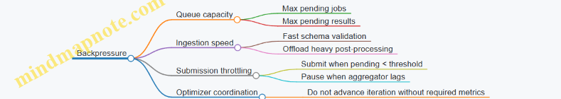
A simple rule works well: allow at most (concurrency + buffer) jobs in flight, where the buffer covers expected parsing time.

Minimal Reference Implementation Pattern

Below is a compact pattern showing three cooperating loops. It’s intentionally framework-agnostic.

# Pseudocode: three-loop throughput pattern
work_queue = Queue(parameters)
pending = {}  # job_key -> job_handle
results_store = {}  # job_key -> parsed_result

while not work_queue.empty() or pending:
    while len(pending) < MAX_CONCURRENT and not work_queue.empty():
        params = work_queue.pop()
        job_key = make_job_key(params)
        if job_key not in results_store:
            pending[job_key] = submit_job(params)

    for job_key, handle in list(pending.items()):
        if handle.is_done():
            raw = handle.get_result()
            parsed = parse_and_validate(raw, job_key)
            results_store[job_key] = parsed
            update_aggregates(parsed)
            del pending[job_key]

This structure prevents submission from blocking on result parsing, while still ensuring each job’s output is validated and aggregated exactly once.

Practical Checklist

• Use deterministic job keys to support idempotent retries.
• Stream results into incremental aggregates weighted by shots.
• Separate submission, ingestion, and work generation loops.
• Apply backpressure by limiting pending jobs and pending results.
• Validate result schema and measurement mapping before updating the optimizer.

These patterns keep the system busy without sacrificing correctness, which is the whole point of throughput: fewer idle cycles, not fewer checks.

11.1 Case Study: Variational Energy Estimation with Qiskit and Cirq

This case study builds a small variational workflow that estimates the ground-state energy of a simple Hamiltonian using a hybrid loop. The same idea appears in both frameworks: prepare a parameterized circuit, measure an observable, compute an energy estimate, then update parameters until the energy stops improving.

Problem Setup

We choose a Hamiltonian written as a weighted sum of Pauli terms:

• \(H = a,Z_0 + b,Z_1 + c,Z_0 Z_1\)

For a two-qubit system, this Hamiltonian is diagonal in the computational basis. That means we can measure energies using only \(Z\)-basis readout, with no basis-rotation logic. This keeps the focus on the hybrid loop and the measurement pipeline.

We use a variational ansatz with two parameters \(\theta_0, \theta_1\):

• Apply \(R_y(\theta_0)\) on qubit 0
• Apply \(R_y(\theta_1)\) on qubit 1
• Add a controlled entangling gate \(\mathrm{CX}(0\rightarrow 1)\)

The ansatz is expressive enough to move probability mass across eigenstates of \(Z\)-type terms.

Mind Map: End to End Variational Loop

Qiskit Implementation Outline

In Qiskit, you typically construct a \(QuantumCircuit\), bind parameters, transpile for the target backend, then run an execution primitive or a sampler-like workflow. For this case study, the key best practice is to keep measurement post-processing explicit so you can verify bit ordering.

Example: build the circuit and compute energy from counts.

from qiskit import QuantumCircuit
from qiskit.circuit import Parameter

th0 = Parameter('th0')
th1 = Parameter('th1')
qc = QuantumCircuit(2)
qc.ry(th0, 0)
qc.ry(th1, 1)
qc.cx(0, 1)

Example: energy computation from counts.

def z_expectation_from_counts(counts, qubit_index, n_qubits=2):
    shots = sum(counts.values())
    exp = 0.0
    for bitstring, c in counts.items():
        # Qiskit bitstrings are ordered as classical register bits.
        # For a 2-qubit circuit with full measurement, bitstring[0] is qubit 1.
        bit = int(bitstring[n_qubits-1-qubit_index])
        z = 1 if bit == 0 else -1
        exp += z * (c / shots)
    return exp

def energy_from_counts(counts, a, b, c):
    z0 = z_expectation_from_counts(counts, 0)
    z1 = z_expectation_from_counts(counts, 1)
    # <Z0 Z1> = average of (z0_i * z1_i) over samples
    shots = sum(counts.values())
    zz = 0.0
    for bitstring, cnt in counts.items():
        b0 = int(bitstring[1])
        b1 = int(bitstring[0])
        z0_i = 1 if b0 == 0 else -1
        z1_i = 1 if b1 == 0 else -1
        zz += (z0_i * z1_i) * (cnt / shots)
    return a*z0 + b*z1 + c*zz

Best practice: before running optimization, test the post-processing on a known state. For instance, if you set \(\theta_0=0\) and \(\theta_1=0\), the circuit prepares \(|00\rangle\) and you should get \(<Z_0>=1\), \(<Z_1>=1\), and \(<Z_0 Z_1>=1\). If your computed energy disagrees, the issue is almost always bit ordering or missing measurements.

Cirq Implementation Outline

Cirq uses moments and explicit measurement operations. The main reliability practice is to keep the measurement key and the qubit-to-bit mapping consistent. In Cirq, you can measure both qubits into a single measurement result array and then compute \(Z\) expectations directly.

Example: build the circuit.

import sympy as sp
import cirq

th0, th1 = sp.symbols('th0 th1')
q0, q1 = cirq.LineQubit.range(2)

circuit = cirq.Circuit(
    cirq.ry(th0)(q0),
    cirq.ry(th1)(q1),
    cirq.CNOT(q0, q1),
    cirq.measure(q0, q1, key='m')
)

Example: compute energy from measurement samples.

import numpy as np

def energy_from_samples(samples, a, b, c):
    # samples shape: (shots, 2) with columns ordered by (q0, q1)
    z0 = 1 - 2*samples[:, 0]
    z1 = 1 - 2*samples[:, 1]
    zz = z0 * z1
    return a*np.mean(z0) + b*np.mean(z1) + c*np.mean(zz)

Best practice: run a quick sanity check with \(\theta_0=0, \theta_1=0\). The measurement samples should be all zeros, producing the same \(<Z\) values as in the Qiskit check.

Hybrid Optimization Loop

Both frameworks share the same loop structure:

1. Start with an initial parameter vector \(\boldsymbol{\theta}\).
2. For each candidate \(\boldsymbol{\theta}\), run the circuit for a fixed shot count.
3. Convert measurement results into \(<Z_0>\), \(<Z_1>\), and \(<Z_0 Z_1>\).
4. Compute energy \(E(\boldsymbol{\theta})\).
5. Update parameters using a classical optimizer.

A practical stopping rule is to stop when the absolute change in energy between iterations is below a small threshold. This avoids spending shots on tiny improvements that are within sampling noise.

What to Verify Before Trusting Results

• Measurement correctness: check \(|00\rangle\) and \(|11\rangle\) cases to confirm \(Z\) sign conventions.
• Parameter binding: ensure the optimizer’s parameters actually reach the circuit (no unused symbols).
• Shot stability: run the same \(\boldsymbol{\theta}\) twice and confirm energy estimates are close enough for the chosen stopping rule.

When these checks pass, the variational loop becomes a straightforward, testable pipeline rather than a black box.

11.2 Case Study: Hybrid Optimization Loop with Reproducible Experiment Logs

A hybrid optimization loop typically alternates between a classical optimizer and a quantum evaluator. The evaluator runs parameterized circuits, returns an objective value, and the optimizer proposes the next parameters. The tricky part isn’t the math; it’s making sure the same inputs produce the same logged outputs, even when execution is asynchronous or involves sampling.

Goal and Setup

We’ll optimize a small parameter vector \(\theta\) to minimize an objective \(f(\theta)\). The objective is computed from measurement data: we run a circuit for \(\theta\), estimate an expectation value, and return \(f(\theta)\) as a deterministic function of the recorded results.

Best practice: treat “objective value” as a computed artifact derived from logged raw results. That way, you can recompute the objective later without rerunning quantum hardware.

Mind Map: Loop Components and Logging Responsibilities

Mind Map: Hybrid Optimization Loop with Reproducible Experiment Logs

Reproducibility Strategy

Use a run ID that ties together everything needed to reproduce a single objective evaluation. A good run ID is derived from:

• A stable serialization of \(\theta\) (fixed precision, fixed ordering)
• The circuit identity (template name or hash)
• Execution settings (shots, backend name, simulator mode)
• Post-processing version (the exact estimator logic)

Then log two layers:

1. Raw layer: counts or quasi-distributions, plus metadata needed to interpret them.
2. Derived layer: expectation value and objective value computed from the raw layer.

If you later change the estimator, you can keep old derived values consistent with the old estimator version.

Example: Parameter Serialization and Run IDs

A common failure mode is parameter ordering. If \(\theta\) is a list but the circuit expects parameters in a different order, you’ll still get numbers—just not the right ones. The fix is to serialize parameters with explicit names and to bind by name.

import hashlib
import json

def stable_theta_payload(theta_dict, precision=10):
    # theta_dict: {"alpha": 0.1, "beta": -0.2, ...}
    payload = {k: round(float(v), precision) for k, v in sorted(theta_dict.items())}
    return payload

def make_run_id(circuit_id, theta_payload, shots, backend_name, estimator_version):
    blob = {
        "circuit_id": circuit_id,
        "theta": theta_payload,
        "shots": shots,
        "backend": backend_name,
        "estimator_version": estimator_version,
    }
    s = json.dumps(blob, sort_keys=True, separators=(",", ":"))
    return hashlib.sha256(s.encode()).hexdigest()[:16]

Example: Logging Structure for One Evaluation

For each objective evaluation, store a single record with:

• run_id
• theta (serialized)
• execution_metadata (backend, shots, transpilation or simulation mode)
• raw_results (counts)
• derived (expectation and objective)
• checks (schema and sanity checks)

def build_log_record(run_id, theta_payload, exec_meta, raw_counts, derived, checks):
    return {
        "run_id": run_id,
        "theta": theta_payload,
        "execution_metadata": exec_meta,
        "raw_results": {"counts": raw_counts},
        "derived": derived,
        "checks": checks,
    }

Example: Objective Computation from Logged Counts

Assume the circuit measures a single qubit in the computational basis after any needed basis rotation. If the observable is \(Z\), then the expectation is:

\(\langle Z \rangle = (P(0) - P(1))\).

Compute \(P\) from counts, then compute objective \(f(\theta)\) as a deterministic function of \(\langle Z \rangle\).

def expectation_z_from_counts(counts):
    shots = sum(counts.values())
    p0 = counts.get("0", 0) / shots
    p1 = counts.get("1", 0) / shots
    return p0 - p1

def objective_from_expectation(exp_z):
    # Example objective: minimize (1 - exp_z)
    return 1.0 - exp_z

Loop Orchestration with Immutable Logs

The classical optimizer calls evaluate(\(\theta\)) repeatedly. Each call must:

1. Bind parameters by name.
2. Submit the quantum job (or run the simulator).
3. Capture raw results and metadata.
4. Compute derived metrics.
5. Validate result schema.
6. Append the immutable record to the log.

A practical validation check is to confirm that the counts keys match the expected measurement bitstrings and that the total shots match the requested shots.

Debugging Notes That Pay Off

• Bit ordering: If you see expectation values with the wrong sign consistently, verify whether your post-processing interprets bitstrings in the same order as the circuit measurement.
• Estimator versioning: If you adjust the objective formula, keep the old derived values tied to the old estimator version.
• Asynchronous execution: Always log after results are retrieved, not when jobs are submitted, so the raw layer matches what actually ran.

Minimal End-to-End Evaluation Record Flow

The loop produces a sequence of records, one per \(\theta\). The optimizer uses only the derived objective value, but the log retains the raw counts and the exact computation rules. That separation makes the optimization trace both useful for debugging and stable for later recomputation.

11.3 Case Study: Observable Measurement Pipeline With Correct Statistical Outputs

This case study builds a small, end-to-end measurement pipeline that produces expectation values with correct uncertainty. The goal is not just “get a number,” but “get a number with a defensible error bar.” We’ll use a simple observable: a single-qubit Pauli Z, measured in the computational basis, and then show how the same pipeline scales to multi-term observables.

Problem Setup

Assume a hybrid loop where classical code repeatedly requests expectation values for different circuit parameters. Each request must:

1. Create or reuse a circuit that measures the observable.
2. Execute on a simulator or backend with a fixed shot budget.
3. Convert raw measurement counts into an expectation value.
4. Compute a standard error that matches the measurement model.

For Pauli Z on one qubit, outcomes are bit values 0 and 1. Map them to eigenvalues: 0 → +1, 1 → −1. If counts are c0 and c1 with N = c0 + c1, then:

• Expectation: \(\langle Z \rangle = (c0 - c1)/N\)
• Variance of a single-shot measurement: \(\mathrm{Var}(Z) = 1 - \langle Z \rangle^2\)
• Standard error: \(\mathrm{SE}(\langle Z \rangle) = \sqrt{\mathrm{Var}(Z)/N}\)

This is the key “correct statistical output” step: the uncertainty depends on the observed expectation, not just on N.

Mind Map: Observable Measurement Pipeline

Example: Single-Qubit Pauli Z from Counts

Suppose a backend returns counts: {'0': 742, '1': 258} with N = 1000.

• \(\langle Z \rangle = (742 - 258)/1000 = 0.484\)
• \(\mathrm{Var}(Z) = 1 - 0.484^2 \approx 0.765\)
• \(\mathrm{SE} \approx \sqrt{0.765/1000} \approx 0.0276\)

A common mistake is using \(\sqrt{1/N}\) regardless of the expectation. That only matches the worst case where \(\langle Z \rangle = 0\). Here, the observed expectation is far from zero, so the uncertainty should shrink.

Minimal Post-Processing Code

import math

def z_expectation_and_se(counts, zero_key='0'):
    c0 = counts.get(zero_key, 0)
    c1 = sum(counts.values()) - c0
    n = c0 + c1
    if n == 0:
        raise ValueError('No shots in counts')

    exp_z = (c0 - c1) / n
    var_z = 1.0 - exp_z * exp_z
    se = math.sqrt(var_z / n)
    return exp_z, se

Example: Basis Rotation for Non-Z Observables

If the observable is Pauli X, you measure in the X basis. For a single qubit, that means applying a Hadamard before measurement, then interpreting the resulting bit values as X eigenvalues. The same counting-to-expectation logic applies after the basis rotation.

A practical best practice is to treat “basis rotation” as part of circuit preparation, not as a post-processing hack. That keeps the mapping between measured bits and eigenvalues explicit.

Mind Map: Multi-Term Observable Aggregation

Example: Two-Term Observable with Independent Shot Sets

Consider \(O = a Z_0 + b Z_1\) measured with separate circuits (or at least separate shot budgets) so the estimates are independent. Suppose you obtain:

• \(\langle Z_0 \rangle = 0.10\), \(\mathrm{SE}_0 = 0.03\)
• \(\langle Z_1 \rangle = -0.40\), \(\mathrm{SE}_1 = 0.02\)

Then:

• \(\langle O \rangle = a(0.10) + b(-0.40)\)
• If independent, variances add: \(\mathrm{Var}(\langle O \rangle) = a^2\mathrm{SE}_0^2 + b^2\mathrm{SE}_1^2\)
• \(\mathrm{SE}_O = \sqrt{a^2\mathrm{SE}_0^2 + b^2\mathrm{SE}_1^2}\)

This is where “correct” matters: linearity gives the expectation, but uncertainty needs variance propagation, not a naive average of errors.

Validation Checks That Prevent Silent Wrong Answers

1. Shot Conservation: sum(counts.values()) must equal the requested shot budget.
2. Eigenvalue Mapping: bit-to-eigenvalue mapping must match the measurement basis used in circuit preparation.
3. Range Check: expectation values for Pauli operators must lie in \([-1, 1]\) up to floating error.
4. Uncertainty Nonnegativity: computed variance must be ≥ 0; clamp tiny negative values caused by rounding.

Output Contract

For each observable request, return a structured result:

• expectation: float
• standard_error: float
• shots: int
• basis: description of measurement basis used
• term_breakdown: optional list of per-term expectations and errors

This contract makes the pipeline usable inside optimizers without forcing them to guess how the numbers were produced.

11.4 Case Study: Cross-Framework Verification Using Shared Reference States

This case study verifies that a hybrid workflow produces consistent results when the same logical circuit is expressed in both Qiskit and Cirq. The key idea is to avoid “equivalent by intention” and instead prove equivalence using shared reference states and shared measurement expectations.

Goal and Verification Strategy

We will:

• Choose a small set of reference input states that are easy to reason about.
• Build the same logical circuit in Qiskit and Cirq.
• Measure the same observables with consistent bit ordering.
• Compare expectation values and, when needed, compare full probability distributions.

A practical rule: if expectation values match for multiple reference states, the measurement pipeline and circuit semantics are likely aligned.

Shared Reference States

Use reference states that cover different behaviors:

• Computational basis states:
• Superposition state:
  • (|00⟩ + |11⟩)/√2

In both frameworks, prepare these states by applying X gates for basis states and H plus controlled operations for the superposition.

The Logical Circuit Under Test

Test a circuit that includes entanglement and a basis change before measurement. For two qubits, one example is:

• Apply H on qubit 0
• Apply CNOT with control qubit 0 and target qubit 1
• Apply a phase-like Z rotation on qubit 1
• Apply a final basis rotation before measurement (e.g., H on qubit 0 for X-basis measurement)

The exact gates are less important than the mix: Hadamard, entangling CNOT, single-qubit phase, and a measurement-basis change.

Measurement Convention Alignment

Cross-framework mismatches often come from bit ordering and basis rotation placement. To prevent that:

• Define a single observable mapping: which qubit index corresponds to which classical bit.
• Apply basis rotations in the circuit itself, not in post-processing.
• Use the same observable definition in both frameworks, such as Z⊗Z, X⊗Z, or X⊗X.

Mind Map: Cross-Framework Verification

Example: Expectation Value from Counts

For an observable like Z⊗Z on two qubits, map each measured bitstring b1b0 to eigenvalue:

• eigenvalue = (+1) if bits are equal, (-1) if bits differ

Then expectation is the weighted average over outcomes.

def zz_expectation_from_counts(counts):
    total = sum(counts.values())
    exp = 0.0
    for bitstring, c in counts.items():
        # Assume bitstring is ordered as q1 q0
        b1 = int(bitstring[0])
        b0 = int(bitstring[1])
        eigen = 1.0 if b1 == b0 else -1.0
        exp += eigen * (c / total)
    return exp

If Qiskit returns bitstrings in a different order than Cirq, swap indices in the mapping or reorder the bitstring before computing eigenvalues.

Example: Cross-Framework Test Harness Logic

Run the same circuit for each reference state and compare expectation values for a small set of observables.

reference_states = ["00", "01", "10", "11", "00_plus_11"]
observables = ["ZZ", "XZ", "XX"]

for state in reference_states:
    qiskit_results = run_qiskit(state, observables)
    cirq_results = run_cirq(state, observables)

    for obs in observables:
        diff = abs(qiskit_results[obs] - cirq_results[obs])
        assert diff < 0.05

The tolerance should reflect shot count. If you use simulators with exact statevectors, you can tighten the threshold.

Debugging When Results Don’t Match

When a mismatch appears, isolate the cause by checking in this order:

1. State preparation: verify that each reference state produces the expected measurement distribution for a simple Z⊗Z measurement.
2. Bit ordering: confirm that the same basis rotation affects the same qubit in both frameworks.
3. Observable mapping: ensure the observable definition matches the measurement basis used in the circuit.
4. Circuit structure: confirm that the entangling gate direction (control/target) matches.

A useful sanity check is to test a circuit that contains only state preparation and a single measurement basis rotation. If that matches, the remaining discrepancy is likely in the tested circuit body.

What “Verified” Means Here

Verification is not “the circuits look similar.” It is “for the shared reference states, the measured expectation values for the chosen observables agree within the expected tolerance.” When that holds, the hybrid application can safely mix Qiskit and Cirq components without silent semantic drift in the parts that matter: state preparation, measurement basis, and observable interpretation.

11.5 Case Study: Robust Execution With Retries, Timeouts, And Validation Checks

Hybrid quantum runs fail in predictable ways: jobs get stuck, networks hiccup, backends reject malformed circuits, and results arrive but don’t match the assumptions your post-processing makes. This case study shows a practical execution wrapper that handles these issues without turning your codebase into a maze.

Mind Map: Robust Execution Flow

Case Study: A Hybrid Evaluator Wrapper

Assume you have a function that evaluates an objective by running a circuit on a backend (or simulator) and computing an expectation value. The wrapper below focuses on execution reliability.

Key design choices

• Retry only when the failure is likely transient (timeouts, temporary network errors, backend “job not found” during propagation).
• Validate before submission so you don’t waste retries on bad inputs.
• Validate after retrieval so you don’t compute nonsense from incomplete results.

Example: Execution Wrapper with Retries and Timeouts

import time

def run_with_retries(executor, submit_fn, validate_pre, validate_post,
                      max_attempts=3, timeout_s=60, backoff_s=2):
    validate_pre()
    last_err = None

    for attempt in range(1, max_attempts + 1):
        try:
            job = submit_fn()
            result = executor(job, timeout_s=timeout_s)
            validate_post(result)
            return result, {"attempt": attempt}
        except Exception as e:
            last_err = e
            msg = str(e).lower()
            transient = any(k in msg for k in ["timeout", "temporar", "network", "rate", "not found"])
            if not transient or attempt == max_attempts:
                raise RuntimeError(f"Execution failed after {attempt} attempts") from e
            time.sleep(backoff_s * attempt)

    raise RuntimeError("Unreachable") from last_err

This wrapper expects three callables:

• validate_pre() checks circuit and parameter completeness.
• submit_fn() submits a job and returns a job handle.
• executor(job, timeout_s=...) fetches results or raises on timeout.
• validate_post(result) checks the result schema and shot consistency.

Preflight Validation That Prevents Useless Retries

A common failure mode is missing parameter bindings. Another is a circuit that doesn’t match the backend’s measurement expectations.

Example: Preflight Checks

def validate_pre_factory(circuit, param_bindings, required_meas_keys):
    def validate_pre():
        missing = [p for p in circuit.parameters if p not in param_bindings]
        if missing:
            raise ValueError(f"Missing parameter bindings: {missing}")
        if not required_meas_keys:
            raise ValueError("No measurement keys specified")
        # Add lightweight structural checks here
    return validate_pre

Post-Result Validation That Catches Silent Mismatches

Even when a job succeeds, you can get results that don’t match your assumptions: wrong measurement key, unexpected shot count, or an empty distribution.

Example: Post-Result Validation

def validate_post_factory(expected_shots, required_meas_keys):
    def validate_post(result):
        if result is None:
            raise ValueError("Result is None")
        if "quasi_dists" not in result and "counts" not in result:
            raise ValueError("Missing distribution data")

        dist = result.get("quasi_dists") or result.get("counts")
        if not dist:
            raise ValueError("Empty distribution")

        shots = result.get("shots")
        if shots is not None and shots != expected_shots:
            raise ValueError(f"Shot mismatch: expected {expected_shots}, got {shots}")

        for k in required_meas_keys:
            if k not in dist:
                raise ValueError(f"Missing measurement key: {k}")
    return validate_post

Putting It Together in a Hybrid Objective

Your objective function should return a normalized value and keep provenance. If validation fails, it should raise an error that includes the attempt count and the last failure reason.

Example: Objective Evaluation Contract

def evaluate_objective(backend_executor, submit_fn, circuit, param_bindings,
                        expected_shots, required_meas_keys):
    validate_pre = validate_pre_factory(circuit, param_bindings, required_meas_keys)
    validate_post = validate_post_factory(expected_shots, required_meas_keys)

    result, meta = run_with_retries(
        executor=backend_executor,
        submit_fn=submit_fn,
        validate_pre=validate_pre,
        validate_post=validate_post,
        max_attempts=3,
        timeout_s=60,
        backoff_s=2
    )

    # Normalize distribution and compute expectation value
    # (Assume you have a separate, tested post-processing function.)
    value = compute_expectation_from_result(result, required_meas_keys)
    return value, {"provenance": meta}

Validation Checklist You Can Actually Use

• Before submission: all parameters bound; measurement keys known; shot count set.
• During execution: timeout enforced; retries only for transient failures.
• After retrieval: distribution exists; measurement keys present; shot count matches expectation.
• On failure: error message includes attempt count and the last underlying exception.

This approach keeps your hybrid loop honest: it either produces a validated value or fails loudly with a reason you can act on.

12.1 Unit Testing Circuit Construction and Parameter Binding

Unit tests for quantum code should answer two questions: “Did we build the circuit we think we built?” and “Did parameter binding produce the values we expect?” The trick is to test structure and semantics without depending on a specific simulator’s quirks.

What to Test

• Circuit structure invariants: number of qubits, number of classical bits (if any), and presence of measurement operations.
• Gate placement invariants: which qubits receive which operations, and whether the order of operations matches your intended layout.
• Parameter schema invariants: parameter names, count, and mapping between symbolic parameters and binding inputs.
• Binding correctness: after binding, no symbolic parameters remain, and the bound values appear in the right places.
• Deterministic serialization: converting the circuit to a stable textual form (or a canonical representation) should be consistent for the same inputs.

Mind Map: Unit Tests for Construction and Binding

Example: Qiskit Parameter Binding Tests

Below is a compact pattern that checks both structure and binding results. The key idea is to inspect the circuit before and after binding, rather than only checking final numeric outputs.

from qiskit import QuantumCircuit
from qiskit.circuit import Parameter


def build_ansatz(n, theta):
    qc = QuantumCircuit(n)
    qc.ry(theta, 0)
    qc.cx(0, 1)
    qc.measure_all()
    return qc


def test_binding_removes_symbols():
    theta = Parameter('theta')
    qc = build_ansatz(2, theta)
    assert qc.num_qubits == 2
    assert len(qc.parameters) == 1

    bound = qc.assign_parameters({'theta': 0.25})
    assert len(bound.parameters) == 0

To verify that the bound value landed on the correct gate, you can search for the operation that uses the parameter and confirm its numeric value.

from qiskit.circuit.library import RYGate


def test_binding_value_on_expected_gate():
    theta = Parameter('theta')
    qc = build_ansatz(2, theta)
    bound = qc.assign_parameters({'theta': 0.25})

    ops = list(bound.data)
    # Expect RY on qubit 0, then CX, then measurements
    assert ops[0][0].name == 'ry'
    assert ops[0][0].params[0] == 0.25

Example: Parameter Key Validation

Binding should fail loudly when keys are wrong. If your code currently accepts missing keys and leaves symbols behind, your tests should catch it.

import pytest


def test_binding_missing_parameter_raises():
    theta = Parameter('theta')
    qc = build_ansatz(2, theta)

    with pytest.raises(Exception):
        qc.assign_parameters({'wrong_name': 0.1}, inplace=False)

Example: Cirq Parameter Binding Tests

Cirq encourages checking the circuit’s moments and the resolved parameter values. A practical approach is to confirm that the circuit contains the expected symbols, then bind and confirm the symbols are gone.

import sympy as sp
import cirq


def build_cirq_ansatz(theta):
    q0, q1 = cirq.LineQubit.range(2)
    return cirq.Circuit(
        cirq.ry(theta).on(q0),
        cirq.CNOT(q0, q1),
        cirq.measure(q0, key='m0'),
        cirq.measure(q1, key='m1'),
    )


def test_cirq_binding_removes_symbols():
    theta = sp.Symbol('theta')
    c = build_cirq_ansatz(theta)
    assert theta in c.all_symbols()

    bound = cirq.resolve_parameters(c, {theta: 0.25})
    assert len(bound.all_symbols()) == 0

Practical Tips That Prevent Common Bugs

• Test qubit indexing explicitly: if your circuit uses qubit 0 for the parameterized gate, assert that directly.
• Test measurement mapping: verify measurement keys or classical bit order so post-processing doesn’t silently swap bits.
• Test “no symbols left”: partial binding is a frequent source of confusing runtime behavior.
• Prefer structural assertions over numeric ones: numeric checks depend on simulator details; structural checks catch mistakes earlier.

A good unit test suite makes it hard to accidentally change the circuit’s meaning while still being fast enough to run every time you touch the code.

12.2 Property-Based Tests for Measurement and Post-Processing Logic

Property-based tests check that your measurement-to-metric pipeline behaves correctly across many inputs, not just a few hand-picked examples. In quantum software, the “inputs” are often raw counts, quasi-distributions, bitstrings, and metadata, while the “outputs” are expectation values, probabilities, and derived features used by optimizers.

What to Test

Start by separating concerns:

• Parsing: converting raw results into a normalized internal representation.
• Bit Ordering: mapping measured bits to qubit indices consistently.
• Basis Rotation: ensuring the measurement basis logic matches the observable definition.
• Aggregation: computing probabilities, expectation values, and variances from samples.
• Edge Cases: empty results, missing keys, zero-shot runs, and malformed bitstrings.

A good property test fails with a small counterexample, so design properties that are specific and checkable.

Mind Map: Measurement Pipeline Properties

Core Properties That Catch Real Bugs

Property 1: Probability Normalization

If you convert counts to probabilities, the probabilities should sum to 1 when shots > 0.

• Generate: random counts over bitstrings of fixed width.
• Assume: total shots > 0.
• Check: sum(p) == 1 within a small tolerance.

This catches mistakes like dividing by the wrong shot total or dropping keys during parsing.

Property 2: Expectation Bounds

For a Pauli-Z-like observable with eigenvalues in {+1, -1}, the expectation value must lie in [-1, 1].

• Generate: random counts.
• Check: computed expectation is within bounds.

This catches sign flips from bit ordering and basis rotation mismatches.

Property 3: Bit Ordering Involution

If you apply a bit-order mapping twice, you should get the original ordering (an involution) when the mapping is its own inverse.

• Generate: random bitstrings.
• Check: map(map(x)) == x.

This is a targeted test for “applied twice” or “applied never” errors.

Property 4: Deterministic Post-Processing

Given the same raw result object, post-processing should return identical outputs.

• Generate: random but fixed inputs.
• Check: repeated calls produce byte-for-byte identical floats when possible, or identical within tolerance.

This catches hidden state, time-dependent behavior, and mutation of shared dictionaries.

Example: Property Tests for Counts to Expectation

Below is a compact example using a Python-style property test approach. The key idea is to generate counts, compute expectation, and assert invariants.

from math import isclose

def counts_to_probs(counts):
    shots = sum(counts.values())
    if shots == 0:
        return {}
    return {b: c / shots for b, c in counts.items()}

def z_expectation_from_probs(probs, bit_index):
    # bit_index: 0 means least-significant bit in the chosen convention
    exp = 0.0
    for bitstring, p in probs.items():
        bit = (int(bitstring, 2) >> bit_index) & 1
        eigen = +1.0 if bit == 0 else -1.0
        exp += eigen * p
    return exp

Now the properties. You can adapt the generator to your test framework.

def prop_prob_sums_to_one(counts):
    probs = counts_to_probs(counts)
    shots = sum(counts.values())
    if shots == 0:
        return probs == {}
    return isclose(sum(probs.values()), 1.0, rel_tol=1e-12, abs_tol=1e-12)

def prop_expectation_in_bounds(counts, bit_index):
    probs = counts_to_probs(counts)
    if not probs:
        return True
    exp = z_expectation_from_probs(probs, bit_index)
    return -1.0 - 1e-12 <= exp <= 1.0 + 1e-12

Example: Bit Ordering Involution Test

If your mapping reverses bitstrings of fixed width, reversing twice returns the original.

def reverse_bits(bitstring):
    return bitstring[::-1]

def prop_reverse_is_involution(bitstring):
    return reverse_bits(reverse_bits(bitstring)) == bitstring

Use this to validate your endianness conversion helper before it touches real measurement data.

Practical Tips for Better Counterexamples

• Constrain generation: fix bit-width and ensure keys are valid bitstrings.
• Prefer small widths: 1–6 qubits produce readable failing cases.
• Make tolerances explicit: floating comparisons should use consistent tolerances.
• Test the parser separately: if parsing fails, post-processing properties become noisy.

Property-based tests are most effective when they target invariants that should never break. When they do break, the smallest counterexample usually points straight at the bug: wrong normalization, flipped bit order, or an observable definition that doesn’t match the measurement basis.

12.3 Debugging Transpilation and Scheduling Mismatches

When a hybrid program “works” in simulation but behaves oddly after transpilation, the culprit is usually not the quantum logic itself. It’s the translation layer: how gates are decomposed, how qubits are mapped, and how operations are ordered under hardware constraints. The fastest debugging approach is to treat transpilation as a deterministic transformation you can inspect, not a black box you hope will behave.

What Mismatches Look Like

Common symptoms include:

• Different measurement distributions after transpilation even with the same shots.
• Unexpected circuit depth or gate counts that change drastically.
• Errors about unsupported operations that appear only on hardware backends.
• Timing-related issues where a circuit that seems valid structurally fails when scheduled.

A useful rule: if the circuit’s intent is stable, then mismatches should correlate with specific compilation steps.

A Debugging Workflow That Actually Narrows the Problem

1. Freeze the input circuit

   • Keep a single source circuit object and avoid rebuilding it with different parameter bindings.
   • Bind parameters once, then transpile the bound circuit.

2. Compare pre- and post-transpile artifacts

   • Compare gate counts, depth, and the set of operations.
   • Compare qubit mapping: which logical qubits ended up on which physical qubits.

3. Inspect decomposition and routing decisions

   • If the backend requires a specific gate basis, check which gates were replaced.
   • If connectivity is limited, check where SWAPs or routing operations were inserted.

4. Check scheduling assumptions

   • Some backends require explicit timing constraints or support only certain parallelism.
   • If the transpiler outputs a scheduled circuit, verify that operations that were assumed independent are not being serialized.

5. Reduce the circuit until the mismatch disappears

   • Remove layers while preserving the failing behavior.
   • The smallest failing circuit is the one you can reason about without spreadsheets.

Mind Map: Where Transpilation Can Change Meaning

Practical Example: Detecting Layout-Induced Changes

Suppose you build a circuit with two logical qubits and expect a specific entangling structure. After transpilation, the entangling gate may be routed through different physical neighbors, which changes the effective circuit under noise.

A debugging pattern is to print the layout and compare it to your expectation.

# Example: compare logical-to-physical layout after transpilation
from qiskit import QuantumCircuit
from qiskit.transpiler import PassManager

qc = QuantumCircuit(2, 2)
qc.h(0)
qc.cx(0, 1)
qc.measure([0, 1], [0, 1])

# Assume `backend` is provided elsewhere
pm = PassManager()  # keep it simple for inspection

# transpile with the backend target
tqc = pm.run(qc) if pm else qc
# In real use, you would call transpile(tqc, backend=backend, ...)
# then inspect tqc.layout and tqc.count_ops() and tqc.depth().

Even without the full backend call shown, the key is what you record: layout, count_ops, and depth. If layout changes, you should expect the physical path for multi-qubit gates to change too.

Practical Example: Isolating Scheduling Serialization

A circuit with commuting operations might appear parallel in a high-level view, but scheduling can serialize them due to resource conflicts or timing constraints. The mismatch shows up as a different scheduled timeline.

A concrete tactic is to compare the unscheduled and scheduled forms and look for operations that move from the same “time layer” to different ones.

# Example: compare scheduled vs unscheduled structure
# Pseudocode style to keep it framework-agnostic

unscheduled = qc
scheduled = schedule_circuit(unscheduled, backend_timing_model)

assert unscheduled.count_ops() == scheduled.count_ops()
assert unscheduled.depth() != scheduled.depth()  # often true

# Inspect timeline or operation ordering
# Look for pairs of gates that were previously independent.

The assertions are intentional: scheduling often preserves the operation multiset but changes ordering and depth.

Invariants and Assertions That Catch Errors Early

Add checks before you run anything expensive:

• Operation set invariant: the transpiled circuit should contain only allowed gate types for the target.
• Measurement mapping invariant: classical bit indices should remain consistent with your measurement intent.
• Qubit count invariant: logical-to-physical mapping should not change the number of qubits.
• Depth sanity check: if depth jumps by an order of magnitude, treat it as a red flag and inspect routing.

A Minimal Checklist for the Next Time It Breaks

• Record layout, count_ops, and depth before and after transpilation.
• Identify whether the mismatch correlates with decomposition, routing, or scheduling.
• Reduce the circuit to the smallest failing example.
• Add invariants so the next failure points to the exact stage.

Debugging transpilation is mostly disciplined comparison. Once you treat each compilation stage as a measurable transformation, the “why” stops being mysterious and starts being a list you can verify.

12.4 Verifying Result Integrity with Schema Checks and Invariants

Hybrid quantum programs fail in boring ways: wrong bit order, missing metadata, mismatched shot counts, or post-processing that quietly assumes a different measurement layout. Result integrity checks catch these issues early by validating structure (schema) and meaning (invariants). The goal is simple: if the output “looks right” but violates a rule, you want a clear error before it contaminates the optimizer loop.

Result Schema Checks That Fail Fast

Treat every returned result as a record with a contract. For each execution, verify:

• Presence: required fields exist (e.g., counts or quasi-distribution, shot count, measurement mapping info).
• Types: counts are numeric, keys are strings or bit-tuples consistently, metadata is a dictionary-like object.
• Ranges: probabilities are within
  • Counts: non-negative integers.
  • Probabilities: between 0 and 1.
• Consistency: totals match shots when counts are used.

A practical pattern is to normalize results into a single internal representation before any computation. For example, convert both frameworks’ outputs into:

• bitstrings: list of observed bitstrings in a chosen order
• counts: aligned list of integers
• shots: integer
• measurement_layout: explicit mapping from circuit measurement wires to bit positions

If you normalize first, your invariants become framework-agnostic.

Invariants That Validate Meaning

Schema checks ensure the shape is correct. Invariants ensure the content matches the circuit and the measurement intent.

Common invariants for hybrid quantum results:

1. Shot Conservation

   • If you have counts, sum(counts) == shots.
   • If you have probabilities, sum(probabilities) == 1 within a tolerance.

2. Key Format and Bit Length

   • Every bitstring key has the expected length equal to the number of measured qubits.
   • No unexpected keys appear (e.g., wrong register size).

3. Measurement Layout Compatibility

   • The result’s bit positions must match the circuit’s measurement mapping.
   • If you reorder bits during post-processing, you must record the mapping and verify it was applied.

4. Observable Term Compatibility

   • If you compute expectation values for specific observables, verify that the measurement basis rotations used to generate the data match the observable evaluation assumptions.

5. Deterministic Metadata for Reproducibility

   • Store a hash of the circuit structure plus the parameter values used for the run.
   • Verify that the hash in the result matches the hash of the request.

Example: Minimal Integrity Validator

The following example shows a compact validator that checks schema and invariants for a counts-based result.

def validate_counts_result(result, expected_measured_qubits):
    required = ["counts", "shots", "measurement_layout"]
    for k in required:
        if k not in result:
            raise ValueError(f"Missing field: {k}")

    counts = result["counts"]
    shots = result["shots"]
    layout = result["measurement_layout"]

    if not isinstance(shots, int) or shots <= 0:
        raise ValueError("shots must be a positive integer")
    if not isinstance(counts, dict) or len(counts) == 0:
        raise ValueError("counts must be a non-empty dict")

    total = 0
    for bitstring, c in counts.items():
        if not isinstance(bitstring, str):
            raise ValueError("count keys must be bitstring strings")
        if len(bitstring) != expected_measured_qubits:
            raise ValueError("bitstring length mismatch")
        if any(ch not in "01" for ch in bitstring):
            raise ValueError("bitstring contains non-binary characters")
        if not isinstance(c, int) or c < 0:
            raise ValueError("counts must be non-negative integers")
        total += c

    if total != shots:
        raise ValueError(f"Shot mismatch: sum(counts)={total}, shots={shots}")

    if not isinstance(layout, dict) or len(layout) == 0:
        raise ValueError("measurement_layout must be a non-empty dict")

    return True

Mind Map: Integrity Checks for Hybrid Results

Example: Catching a Subtle Bit-Order Bug

Suppose you compute an expectation value from counts but accidentally reverse bit order during normalization. The schema still passes: keys are binary strings of the right length, and shots match. The invariant that catches the issue is measurement layout compatibility.

A robust approach is to store an explicit mapping like measurement_layout = {"wire": [0,1,2], "bit_positions": [2,1,0]} and verify that the normalization step used that mapping. If the mapping is missing or inconsistent, fail before computing expectation values.

Example: Invariant-Driven Optimizer Safety

In a hybrid loop, you typically update parameters based on computed objective values. Add a rule: if validation fails, do not return an objective value. Instead, raise an exception or return a structured error that the optimizer wrapper treats as “no update.” This prevents a single malformed result from nudging parameters in the wrong direction.

Result integrity checks are not glamorous, but they are effective: they turn silent mismatches into immediate, actionable failures, and they keep your classical loop honest about what the quantum data actually means.

12.5 Building a Minimal Reproducible Experiment Harness for Hybrid Runs

A minimal reproducible experiment harness is a small, boring program that can rerun the same hybrid quantum job and produce the same artifacts: inputs, circuit parameters, execution settings, raw results, and computed outputs. “Minimal” means you remove everything that isn’t needed to reproduce one run end-to-end.

Goals and Non-Goals

Goals

• Capture every knob that affects results: seed, shot count, noise model choice, transpilation options, and measurement mapping.
• Produce stable artifacts: a run manifest, a serialized circuit representation, raw counts or samples, and a computed summary.
• Fail loudly when something changes: mismatched parameter schemas, missing metadata, or incompatible result formats.

Non-Goals

• Building a full workflow engine.
• Hiding framework differences behind magic.
• Optimizing performance before correctness.

Mind Map: Minimal Harness Components

Run Manifest: The “One File to Rule Them All”

Use a single JSON manifest that records the exact configuration. Keep it small but complete. A good manifest includes a parameter schema so you can detect accidental reordering.

Example: manifest.json

{
  "experiment_id": "mre-001",
  "seed": 1234,
  "shots": 4096,
  "backend": "qasm_simulator",
  "noise_model": "none",
  "transpile": {"optimization_level": 1},
  "parameter_schema": ["theta", "phi"],
  "parameters": {"theta": 1.234, "phi": 0.5},
  "measurement_mapping": {"qubit_order": [0, 1, 2]},
  "framework": {"qiskit": "x.y.z", "cirq": "a.b.c"}
}

Circuit Serialization and Hashing

You want a stable way to confirm you ran the same circuit structure. Serialize a framework-agnostic representation when possible, or at least store a framework-specific dump plus a hash.

Example: circuit.json fields

• circuit_type: “qiskit” or “cirq”
• parameter_names: ordered list
• gate_sequence: a compact list of operations
• measurement_map: which qubit index becomes which classical bit
• structure_hash: computed from the serialized gate sequence and measurement map

A structure hash catches the common bug where you changed a gate order or measurement mapping but kept the same parameter values.

Execution Wrapper with Strict Validation

The harness should validate inputs before running and validate outputs after running.

Example: minimal Python harness skeleton

import json, hashlib
from dataclasses import dataclass

@dataclass
class RunConfig:
    seed: int
    shots: int
    parameters: dict
    parameter_schema: list

def schema_check(cfg: RunConfig):
    assert list(cfg.parameters.keys()) == cfg.parameter_schema

def structure_hash(gate_sequence, measurement_map):
    payload = json.dumps({"gates": gate_sequence, "meas": measurement_map}, sort_keys=True)
    return hashlib.sha256(payload.encode()).hexdigest()

def run_hybrid(cfg: RunConfig, build_circuit, execute, postprocess):
    schema_check(cfg)
    circuit_repr = build_circuit(cfg.parameters)
    raw = execute(circuit_repr, cfg)
    summary = postprocess(raw)
    return circuit_repr, raw, summary

Example: Deterministic Behavior Checks

Determinism is tricky because sampling introduces randomness. Still, you can check determinism where it exists.

• For simulators that support seeding, rerun with the same seed and confirm raw counts match exactly.
• If you use a noise model, ensure the noise model is identified in the manifest and that its internal seed is controlled.

Example: deterministic check logic

def assert_same_raw(raw1, raw2):
    # raw1/raw2 are dicts like {"00": 123, "01": 45, ...}
    assert raw1 == raw2

# Run twice with same cfg
c1, r1, s1 = run_hybrid(cfg, build_circuit, execute, postprocess)
c2, r2, s2 = run_hybrid(cfg, build_circuit, execute, postprocess)
assert_same_raw(r1, r2)

Artifact Layout and Naming

Store artifacts in a run-specific folder named by experiment_id plus a short suffix. Keep filenames stable so scripts can find them.

Recommended files

• manifest.json
• circuit.json
• raw_results.json
• summary.json
• validation.json

Example: validation.json

• schema_ok: true/false
• structure_hash_match: true/false
• measurement_mapping_ok: true/false
• deterministic_raw_match: true/false

Minimal Example Workflow

1. Create manifest.json with parameters, seed, shots, and measurement mapping.
2. Build the circuit from the manifest parameter schema.
3. Compute and store structure_hash.
4. Execute and store raw_results.json exactly as returned.
5. Post-process into summary.json with computed metrics and uncertainty.
6. Run validation checks and write validation.json.

If any step changes, the harness either updates the artifacts intentionally or fails validation. That’s the whole point: reproducibility without relying on memory.