Enterprise Profitability Analysis
1. Foundations of Profitability Analysis for Enterprises
1.1 Defining Profitability Objectives and Decision Use Cases
Profitability analysis is not a single report; it is a set of decisions supported by consistent numbers. The first step is to define what “better” means for your enterprise and which decisions those numbers must improve. If you skip this, you’ll end up with dashboards that look impressive and answer none of the questions people actually ask in meetings.
Start with Decision Questions, Not Metrics
A good objective is tied to a decision that has a clear owner, a timing cadence, and a measurable outcome. For example:
- Objective: Improve profitability of a product line.
- Decision use case: Approve a price change for SKU groups.
- What must be answered: How much margin changes after volume and discount effects.
- Objective: Reduce cost-to-serve without harming service levels.
- Decision use case: Redesign fulfillment routes and carrier mix.
- What must be answered: Which customers or regions drive the most cost per order.
- Objective: Improve profitability of customer relationships.
- Decision use case: Decide whether to renew a contract.
- What must be answered: Expected contribution after rebates, returns, and support costs.
Notice the pattern: each objective implies a “because of X, we will do Y” logic. Metrics come after that logic.
Translate Objectives into Profit Views
Enterprises rarely agree on one profitability number because different decisions need different views. Common views include:
- Contribution margin view: Useful for pricing, promotions, and deal approvals because it isolates revenue less directly attributable variable costs.
- Segment margin view: Useful for product, customer, and channel decisions because it includes allocated operating costs that are meaningful at that segment level.
- Operating profit view: Useful for budgeting and performance management because it reflects broader cost structure and normalization choices.
A practical best practice is to define a “minimum viable set” of views for the first rollout. For instance, if the immediate pain is discounting and deal profitability, start with contribution margin and a simple cost-to-serve layer, then expand.
Define the Decision Boundary and Time Horizon
Profitability numbers change depending on what you include and when you measure it.
- Decision boundary: Are you evaluating a one-time promotion, a contract term, or a full fiscal year?
- Time horizon: Are you measuring immediate margin impact, or margin plus working capital effects like receivables and inventory?
Example: A sales team proposes a 10% discount for 60 days. If you evaluate only gross margin, you may miss that the promotion increases returns and slows inventory turns. Adding a working-capital-aware view for that decision prevents “margin today, cash later” surprises.
Specify Inputs and Assumptions Up Front
Every profitability objective requires assumptions. The goal is not to guess perfectly; it is to make assumptions explicit and consistent.
Key assumption categories:
- Volume behavior: How price changes affect units.
- Cost behavior: Which costs scale with volume and which do not.
- Commercial terms: Discounts, rebates, returns, and service fees.
- Allocation rules: How shared costs are assigned to segments.
A simple example: If you allocate customer support costs by number of tickets, define what counts as a ticket and how to treat merged cases. Otherwise, the model will “work” but produce inconsistent results month to month.
Mind Map: Objectives to Use Cases to Required Outputs
Example: Turning a Vague Goal into a Usable Objective
Vague: “We want better margins.”
Systematic rewrite:
- Objective: Increase enterprise contribution margin by improving deal economics.
- Decision use case: Approve discount requests above the standard threshold.
- Required outputs:
- Contribution margin per deal line item.
- Expected volume change from discount level.
- Treatment of rebates and returns in the same calculation.
- Assumptions to define: discount-to-volume relationship, variable cost rates, and whether returns are modeled as a percentage of shipped units.
If you can’t list these items, you don’t yet have an objective—you have a wish.
Quick Checklist for Objective Definition
- Is the objective tied to a specific decision?
- Does the objective specify the profit view needed for that decision?
- Are the decision boundary and time horizon explicit?
- Are the key assumptions and allocation rules defined at the start?
- Can someone else reproduce the same numbers from the same inputs?
When these answers are clear, the rest of the profitability analysis becomes much easier: you can build models that explain outcomes instead of merely reporting them.
1.2 Mapping Profit Drivers Across Revenue Cost and Operating Expenses
Profitability improves when you can point to the specific levers that move it. Mapping profit drivers means translating financial line items into a structured set of causes: what changes revenue, what changes costs, and what changes operating expenses. The goal is not to create a perfect model on day one; it is to build a driver map that is consistent, explainable, and usable for decisions.
Profit Drivers as a Layered System
Start with a simple layer model:
- Revenue drivers explain how much you sell and at what economics.
- Cost drivers explain what it costs to deliver what you sold.
- Operating expense drivers explain how the business runs day to day.
A practical rule: every driver should have a measurable input and a clear direction of impact. If you cannot name the input (for example, “units shipped” or “labor hours”), the driver is probably too vague.
Revenue Drivers
Revenue is usually driven by volume, price, and mix. Mix matters because different products, customers, or channels can carry different margins and service requirements.
- Volume: units sold, active customers, trips, seats, or transactions. Example: if a retailer sells 10,000 units instead of 9,000, revenue rises, but margin may not if returns or logistics costs scale differently.
- Price: list price, realized price, or net price after discounts. Example: a 2% price increase can be offset by higher discounting elsewhere, so you track realized price by segment.
- Mix: product mix, customer mix, channel mix. Example: shifting sales from a high-margin SKU to a low-margin SKU can reduce gross margin even if total revenue stays flat.
Cost Drivers
Costs typically split into direct costs (tied to delivery) and indirect costs (tied to capacity, complexity, or overhead). Mapping requires deciding where each cost belongs.
- Direct material and labor: driven by units and production hours. Example: if labor is partly overtime, cost per unit can jump when volume crosses a threshold.
- Fulfillment and logistics: driven by shipment count, weight, distance, and service level. Example: faster delivery increases carrier cost per shipment and may also increase customer returns.
- Returns and allowances: driven by return rate and processing cost. Example: a promotion can increase returns if it attracts customers with higher defect or mismatch rates.
A useful technique is to tag each cost line with a “primary driver” and a “secondary driver.” Primary is what explains most of the variation; secondary explains the rest.
Operating Expense Drivers
Operating expenses often behave differently from direct costs. They may scale with headcount, transactions, or business complexity.
- Sales and marketing: driven by leads, campaigns, sales coverage, and conversion rates. Example: higher spend can raise revenue, but you still map it to the revenue drivers it influences.
- General and administrative: driven by number of entities, employees, or process volume. Example: finance close effort can rise with more SKUs and more frequent reporting.
- R&D and product development: driven by project counts, engineering hours, or roadmap scope. Example: expanding a product line increases testing and documentation costs even before revenue arrives.
To keep the map decision-ready, define boundaries: operating expenses should not silently absorb costs that belong in cost-to-serve. If you do not set boundaries, your driver map will “explain” everything and therefore explain nothing.
Mind Map: Profit Driver Mapping
Example Mapping in Practice
Assume a subscription business with these simplified financial lines:
- Revenue: net subscription revenue
- Cost of revenue: hosting and support
- Operating expenses: sales salaries and customer success management
A driver map might look like this:
- Revenue
- Volume: active subscribers
- Price: realized monthly fee after discounts
- Mix: plan tier distribution
- Cost of revenue
- Hosting: compute usage per active subscriber
- Support: support tickets per active subscriber
- Operating expenses
- Sales salaries: sales headcount and pipeline conversion
- Customer success: churn reduction effort measured by churn rate changes
Notice the discipline: customer success is mapped to churn and retention, not just to “more people.” That keeps the driver map aligned to outcomes.
From Drivers to a Profit Bridge-Friendly Structure
Once drivers are mapped, you can connect them to a profit bridge. Gross margin moves with revenue drivers and cost-to-serve drivers; operating profit moves with gross margin plus operating expense drivers. The bridge becomes easier because each driver already has a measurable input and a defined financial destination.
1.3 Selecting Profit Metrics and Establishing Calculation Consistency
Profitability analysis fails in two predictable ways: teams pick metrics that answer different questions, or they compute the same metric differently across time, segments, and models. This section fixes both by treating metric selection and calculation consistency as one system.
Start with Decision Questions, Not Metric Lists
Choose metrics by mapping them to decisions.
- Product and customer decisions need margin that reflects what you keep after direct costs.
- Channel and territory decisions need contribution that accounts for cost to serve.
- Management performance decisions need operating profit that includes overhead in a controlled way.
A practical rule: if a metric cannot be tied to a specific action, it will become a dashboard decoration.
Build a Metric Ladder from Revenue to Profit
Use a ladder so each step explains the next.
- Revenue: what came in.
- Gross Margin: revenue minus direct product costs.
- Contribution Margin: gross margin minus variable and directly traceable costs.
- Segment Operating Profit: contribution minus allocated operating expenses.
- Net Income: segment operating profit plus non-operating items and taxes.
Example: A retailer sells a bundle.
- Revenue: $1,000
- Direct product cost: $600 → Gross margin $400
- Shipping and payment fees tied to orders: $120 → Contribution $280
- Store labor and rent allocated to the store: $200 → Segment operating profit $80 If you skip steps, you cannot tell whether the problem is product cost, fulfillment, or overhead.
Define Metric Components with Explicit Rules
For each metric, document four things: scope, inclusions, exclusions, and allocation method.
- Scope: which business unit, time period, and currency.
- Inclusions: which line items are allowed.
- Exclusions: what is intentionally left out.
- Allocation method: how shared costs are assigned, if at all.
Example rules that prevent confusion:
- Gross margin includes only product-related direct costs.
- Contribution includes order-level costs (shipping, payment processing) but excludes marketing brand spend.
- Segment operating profit allocates store rent using square footage, not headcount.
Establish Calculation Consistency Across the Enterprise
Consistency means the same metric means the same thing everywhere.
Key practices:
- Single source of definitions: one metric dictionary used by finance, analytics, and reporting.
- Same sign conventions: revenue positive, costs negative (or vice versa) but never mixed.
- Same period logic: accruals and reversals follow the same cut-off rules.
- Same currency treatment: either translate at transaction date or reporting date, but do not mix within a metric.
- Same rounding and tolerance: define acceptable reconciliation gaps (for example, within $1 due to rounding).
A quick check: if Gross Margin for a segment changes when you re-run the report with the same filters, the model has hidden dependencies.
Use a Mind Map to Keep Metrics and Rules Aligned
Mind Map: Profit Metrics and Consistency Rules
Handle Discounts, Returns, and Allowances Without Breaking the Ladder
These items are where metric definitions often drift.
Example: A $1,000 list-price sale has a $100 discount and a $30 return allowance expected.
- If you subtract discounts from revenue, revenue becomes $900.
- If you subtract discounts from gross margin, revenue stays $1,000 and gross margin reduces. Either can work, but the ladder must remain internally consistent.
Best practice: decide where each component lands based on how you want to manage it.
- If sales leaders control discounting, keep it in the revenue-to-gross-margin step.
- If returns are driven by product quality, keep them in the gross margin step.
Example: A Consistent Metric Set for One Segment
Assume one segment, one month.
- Revenue: $1,000
- Direct product cost: $600
- Order shipping and payment fees: $120
- Store rent allocated by square footage: $200
Computed metrics:
- Gross Margin = 1,000 − 600 = $400
- Contribution Margin = 400 − 120 = $280
- Segment Operating Profit = 280 − 200 = $80
Now apply consistency checks:
- Re-running with the same filters must reproduce $80.
- Segment roll-up must equal the sum of its subsegments within the defined rounding tolerance.
- Gross Margin must reconcile to the income statement view using the documented inclusion/exclusion rules.
A Minimal Calculation Template to Reduce Drift
Use a template that forces the same structure every time.
Metric: Contribution Margin
Inputs:
- Revenue
- Direct product costs
- Order-level variable costs
Rules:
- Contribution = (Revenue - Direct product costs) - Order-level variable costs
- Discounts and allowances follow the agreed revenue or gross margin placement
- Costs use the same sign convention across all segments
Validation:
- Profit ladder reconciliation passes
- Segment roll-up within rounding tolerance
When metric selection and calculation rules are treated as a single design task, profitability analysis becomes comparable, explainable, and—most importantly—trustworthy enough to support decisions.
1.4 Building a Profitability Data Model from Source Systems
A profitability data model is the bridge between accounting truth and decision usefulness. The goal is simple: every margin number you show should be reproducible from source transactions, with clear rules for what gets included, excluded, and allocated.
Start with Profitability Grain and Questions
Begin by choosing the “grain,” meaning the smallest unit your model stores. Common grains are:
- Order line for deal and pricing analysis
- Shipment line for cost to serve
- Customer-month for collections and working capital views
- Product-customer-channel for margin waterfalls
Then write the questions the model must answer. If you need “margin by customer and channel,” your grain must support those dimensions without forcing guesswork. A model that stores only monthly totals can still show profitability, but it will struggle to explain why it changed.
Inventory Source Systems and Their Roles
List each source system and what it contributes. Typical inputs include:
- Billing and invoicing for revenue and discounts
- Order management for quantities, terms, and product identifiers
- Finance general ledger for accounting totals and reconciliation targets
- Procurement and logistics for freight, warehousing, and handling
- Master data for product hierarchy, customer hierarchy, and channel definitions
A practical rule: treat master data as the “naming layer,” and treat transactions as the “number layer.” Mixing them early creates confusion later.
Define Canonical Entities and Keys
Your model needs stable identifiers that survive system quirks. Create canonical entities such as:
- Customer
- Product
- Order
- Invoice
- Shipment
- Cost event
- Period
Use keys that can be traced back to source IDs. For example, an invoice line should carry both the invoice ID and the originating order line ID. If you cannot trace, you will eventually allocate instead of calculate.
Build a Revenue and Cost Fact Structure
Use fact tables for measurable events and dimension tables for descriptive attributes.
- Revenue fact: invoice line amounts, quantities, and discount components
- Cost fact: direct costs tied to orders, shipments, or cost events
- Allocation fact: intermediate results used to distribute indirect costs
Keep measures consistent in sign and units. If revenue is positive and costs are positive, store costs as positive and compute profit as revenue minus costs. If you store costs as negative, document it once and enforce it everywhere.
Create Allocation Rules as First-Class Logic
Indirect costs rarely “belong” to a single transaction, so you need allocation rules that are explicit and testable. Each allocation rule should specify:
- Source pool: what total is being allocated
- Driver: what basis spreads the pool (labor hours, shipments, square footage, etc.)
- Scope: which segments are eligible
- Timing: when the allocation happens (invoice date, shipment date, or accounting period)
A good model stores allocation outputs so reports don’t re-run complex logic differently.
Reconcile to Accounting Totals Without Losing Detail
Profitability models should reconcile to the general ledger at a defined level. A common approach is:
- Reconcile revenue totals by period
- Reconcile direct cost totals by period
- Reconcile indirect cost pools by period
Then allow segment-level reporting to be more granular than the ledger. If reconciliation fails, fix the mapping or rules, not the report.
Handle Adjustments and Exceptions Systematically
Adjustments include returns, credits, rebates, and write-offs. Decide where they land:
- Revenue adjustments should reduce the revenue fact tied to the original sale when possible
- Cost adjustments should reduce or increase the relevant cost pool when traceability exists
If traceability is missing, allocate adjustments using a driver that matches the business logic. For example, a credit issued after a return should reduce margin for the returned product and customer if you can identify them.
Mind Map: Data Model Components and Flow
Example: From Invoice Lines to Profit by Product and Customer
Suppose you want margin by product and customer for March. Your model might work like this:
- Revenue fact stores invoice line net amounts after discounts, plus quantity.
- Direct cost fact stores freight and handling tied to shipments that correspond to those invoice lines.
- Indirect cost pools store totals for warehousing overhead and customer service overhead for March.
- Allocation rules distribute warehousing overhead using square footage-days, and customer service overhead using service tickets.
- Profit is computed as: net revenue minus direct costs minus allocated indirect costs.
If March ledger revenue is 100,000 but your revenue fact sums to 99,200, you investigate mapping gaps or missing invoices. Once the totals reconcile, the product-customer breakdown becomes trustworthy.
Example: Allocation Rule Test Case
Create a test case for one indirect pool. For instance, allocate customer service overhead:
- Pool total for March: 40,000
- Driver total for eligible customers: 2,000 tickets
- Customer A tickets: 120
- Allocated amount for Customer A: 40,000 × (120 / 2,000) = 2,400
Store the driver totals used for the calculation. When someone asks why Customer A moved by 300 next month, you can point to the driver change or scope change rather than “re-running the model and hoping.”
Diagram: End-to-End Data Flow
    flowchart LR
  A[Source Transactions] --> B[Staging and Standardization]
  B --> C[Canonical Entities and Keys]
  C --> D[Fact Tables]
  D --> E[Allocation Rules and Pools]
  E --> F[Profit Measures]
  F --> G[Reconciliation to Ledger]
  G --> H[Reporting Views]
  D --> I[Adjustments Handling]
  I --> F
A solid profitability data model is less about cleverness and more about discipline: clear grain, traceable keys, explicit allocation logic, and reconciliation that catches problems early. When those pieces are in place, margin reporting becomes explainable rather than mysterious.
1.5 Establishing Governance for Definitions Controls and Auditability
Profitability analysis breaks when definitions drift. Governance is the set of rules that keeps “margin” meaning the same thing across finance, sales finance, operations, and reporting. The goal is simple: when someone asks why a segment’s profit changed, you can trace the answer to a specific definition, a specific transformation, and a specific approval.
Start with a Definition Catalog That People Can Actually Use
Create a definition catalog that lists each metric and its inputs, calculation logic, and scope. For example, define Gross Margin as:
- Revenue: net of customer rebates and returns
- Cost of goods sold: includes freight-in if your policy says so
- Exclusions: excludes internal transfers
A practical rule: every definition must include “what’s in,” “what’s out,” and “what to do when data is missing.” If freight-in is sometimes missing, specify whether you use a default rate, exclude the cost, or flag the record.
Set Metric Ownership and Change Rights
Governance fails when everyone can change formulas. Assign an owner for each metric (usually finance) and define who can request changes (often business users) and who can approve them (metric owner plus a data steward). Use a lightweight workflow with a change ticket that records:
- Metric and version
- Reason for change
- Impacted reports and segments
- Effective date
Example: If you decide to include credit card processing fees in operating expenses instead of revenue deductions, you approve the definition change, then re-run historical periods only if the business requires comparability.
Build Controls Around Data Inputs and Transformations
Controls should cover both data quality and logic correctness.
Input controls check that required fields exist and are within expected ranges. Example: unit quantity must be positive for sales lines; if returns are stored as negative quantities, the control must reflect that.
Transformation controls verify that joins and allocations behave as intended. Example: when allocating shared logistics costs to channels, confirm that the allocation base totals match the source pool totals within a tolerance.
Output controls ensure the final numbers reconcile to the accounting view. A reconciliation is not just a “nice-to-have”; it’s the audit trail that proves the analytical model is anchored.
Enforce Calculation Consistency with Versioned Logic
Versioning prevents silent drift. Store calculation logic with a version number and link it to the definition catalog. When a report is published, it should reference the exact logic version used.
A concrete example: you might change the treatment of discounts from “netting against revenue” to “separating discount revenue.” Even if the final margin looks similar, the path matters for auditability.
Make Auditability a Trace from Metric to Source
Auditability means you can answer three questions quickly:
- Which definition produced the number?
- Which data and transformations were applied?
- Which approvals authorized the logic?
To support this, capture lineage at the field level where feasible: source table → transformation → intermediate staging → final metric. If full field-level lineage is too heavy, at least capture lineage at the dataset level and record allocation rules and mapping tables.
Document Exceptions Without Hiding Them
Not all data will be perfect. Governance requires an exception policy that specifies how to handle missing mappings, unknown customers, and unmatched cost pools.
Example: If a customer segment mapping is missing for 0.5% of transactions, route those transactions to an “Unmapped” bucket and report the percentage. Don’t quietly assign them to the largest segment; that makes the model look cleaner than reality.
Use a Simple Evidence Pack for Reconciliations
For each reporting cycle, produce an evidence pack that includes:
- Reconciliation summary between accounting and analytical totals
- Control results (input, transformation, output)
- List of exceptions and how they were treated
- Approved definition and logic versions
This pack should be generated consistently, not assembled from memory.
Mind Map: Governance for Definitions, Controls, and Auditability
Example Control Set for a Margin Report
Example controls for a monthly margin report:
- Input control: verify total sales quantity equals sum of line items after returns sign handling.
- Transformation control: confirm allocation base totals match the cost pool totals within 0.1% tolerance.
- Output control: reconcile analytical revenue and COGS to accounting totals; investigate any variance above a defined threshold.
- Audit control: ensure the report references the approved definition version and logic version.
If a variance appears, the evidence pack should point to the exact control that failed and the exact rule that was applied. That’s governance doing its job: fewer debates, more traceable answers.
2. Financial Statement Structures and Profit Bridge Mechanics
2.1 Understanding Income Statement Line Items and Their Analytical Meaning
An income statement is a structured story of how a business turns activity into profit. For profitability analysis, the key is to understand what each line item actually represents, what it includes, what it excludes, and how it behaves when you change assumptions like volume, price, or cost-to-serve.
The Income Statement as a Profit Path
Start with the top of the statement: revenue. Revenue is the amount recognized for sales during the period, after applying contract terms and revenue recognition rules. Analytical meaning matters because revenue can be affected by timing (when recognition occurs) and by netting (for example, whether certain deductions are recorded as revenue reductions or as separate expense lines).
Next comes gross profit. Gross profit typically equals revenue minus cost of goods sold (COGS). COGS is where many “direct” costs live: materials, direct labor, and manufacturing overhead allocated to products. In analysis, gross profit is often the first place where margin intelligence becomes practical, because it ties directly to product economics.
Operating expenses follow. These are costs required to run the business beyond producing goods or delivering services. They are usually split into categories such as selling, general and administrative (SG&A), research and development (R&D), and other operating expenses. For profitability analysis, the analytical challenge is that operating expenses are often not naturally “owned” by a single product or customer, so you must interpret them carefully before allocating them.
Finally, you reach operating income, then other income and expenses, then net income. Other items can include interest, taxes, and non-operating gains or losses. These lines are important for completeness, but they often do not map cleanly to day-to-day margin drivers.
Line Item Meaning by Level of Analytical Use
A useful way to classify income statement lines is by how directly they connect to controllable drivers.
- Driver-close lines: revenue, COGS, and many direct fulfillment costs. These respond predictably to volume, price, and operational throughput.
- Driver-intermediate lines: operating expenses like sales commissions, customer support, and logistics-related costs if they are tracked there. These may respond to activity levels, but definitions vary.
- Driver-far lines: interest expense, taxes, and certain non-recurring items. These can distort comparisons if you mix them into margin views.
A practical rule: if a line item is not tied to a controllable operational driver, treat it as a separate layer in your analysis rather than forcing it into the same margin story.
Mind Map: Income Statement Lines and Analytical Implications
Concrete Examples That Keep Definitions Honest
Example 1: Revenue deductions placement. Suppose a company sells equipment for $1,000,000 and offers $50,000 in rebates that are expected to be earned. If rebates are recorded as a reduction of revenue, then analytical revenue is $950,000 and gross margin is computed on that net figure. If instead rebates are recorded later as an expense, revenue stays $1,000,000 and gross margin looks higher until the rebate expense hits. The profitability model must follow the accounting reality or normalize consistently.
Example 2: COGS includes overhead allocations. A manufacturer may include plant overhead in COGS. If overhead allocation uses a standard rate based on machine hours, then COGS will change with production volume even when direct materials stay stable. In analysis, you can still use gross margin, but you should remember that “direct” margin is partly influenced by utilization.
Example 3: Operating expense categories hide cost-to-serve. A retailer might record customer support costs in SG&A. If support volume is driven by returns and order complexity, then SG&A contains a cost-to-serve component. For profitability analysis by customer or channel, you may need to reclassify or allocate parts of SG&A using measurable activity drivers.
Analytical Takeaways for the Next Steps
When you interpret income statement lines, you are really answering four questions: what the line includes, what it excludes, how it is measured, and how it relates to the drivers you want to explain. Once those answers are clear, you can build profit bridges and segment profitability without accidentally mixing accounting artifacts into operational margin signals.
2.2 Interpreting Balance Sheet Impacts on Profitability Through Working Capital
Profitability is often treated like a purely income-statement story: revenue minus costs. Working capital reminds you that profit can be “earned” on paper while cash is still stuck in receivables, inventory, or payables. Interpreting the balance sheet through working capital connects the two views so you can explain why margins and cash move together—or don’t.
Working Capital as the Bridge Between Profit and Cash
Working capital is the net of current assets and current liabilities used to run the business day to day. A simple starting point is:
- Net Working Capital (NWC) = Current Assets − Current Liabilities
- Cash Conversion Cycle (CCC) = Days Inventory + Days Receivable − Days Payable
The key idea: changes in working capital can absorb or release cash without changing revenue or expense immediately. That’s why two companies with similar margins can show different cash performance.
Receivables and the Timing Gap
Receivables represent sales you’ve recognized but haven’t collected yet. When receivables rise faster than revenue, you’re effectively financing customers.
Example: A distributor reports steady gross margin. In the same quarter, revenue is flat, but days sales outstanding increases from 35 to 45. The income statement may show the same profit, yet cash is lower because 10 extra days of sales are sitting in invoices.
To interpret this, compare:
- Receivables growth vs. revenue growth
- Aging buckets (current, 1–30, 31–60, 61–90)
- Collection patterns by customer segment
If aging shifts toward older buckets, the issue is not just timing; it can signal credit risk or billing disputes.
Inventory and the Cost of Holding Things
Inventory ties up cash and can also create accounting effects that hit profitability. Holding inventory longer increases storage, handling, and obsolescence risk. It can also lead to write-downs that reduce gross margin.
Example: A consumer electronics retailer keeps pricing stable. Gross margin looks fine, but inventory turns slow down. The company eventually records s, lowering gross margin in later periods. The balance sheet change is the early warning; the income statement impact may arrive after.
Interpret inventory changes by separating:
- Volume effects (more units purchased)
- Mix effects (more slow-moving SKUs)
- Process effects (forecast accuracy, replenishment rules)
A helpful check is to compare inventory value changes with sales volume changes. If inventory rises while sales units fall, you likely have a demand mismatch.
Payables and Supplier Financing
Payables represent obligations to suppliers. Extending payment terms can release cash, but it can also strain supply continuity or trigger higher costs.
Example: A manufacturer negotiates longer terms from 30 to 45 days. Profitability on the income statement may remain stable, while operating cash improves because cash is held longer. However, if suppliers respond with higher unit prices or reduced shipment reliability, future gross margin can deteriorate.
Interpret payables using:
- Payables days and trend consistency
- Purchase volume vs. payables growth
- Any changes in supplier terms that explain the movement
Net Working Capital Changes and Profitability Quality
A practical way to connect the balance sheet to profitability is to analyze the difference between accounting profit and cash from operations. When working capital increases, cash from operations often falls relative to profit.
Example: A software company shows positive operating profit. Yet cash from operations is weak because receivables increase due to longer collection cycles. The company’s profitability is real, but its profitability quality is lower in the short term because cash is delayed.
To keep this systematic, use a working capital bridge:
- Start with operating profit
- Adjust for non-cash items
- Then adjust for changes in receivables, inventory, and payables
The bridge tells you whether the profit is “cash-backed” or “cash-lagged.”
Mind Map: Working Capital Pathways to Profit
Advanced Interpretation: Separating Structural vs Temporary Effects
Not every working capital movement is a problem. Some are structural (new customer terms, product mix) and some are temporary (one-off billing cycles, seasonal inventory).
Example: A retailer experiences seasonal demand. Inventory rises before peak season, then falls after. Profit may be stable, and cash improves later. If you treat the pre-season build as a permanent issue, you’ll chase the wrong lever.
To separate these, compare the current period to:
- The same period in the prior year
- The trailing average for the same season
- Internal operational metrics like shipment schedules and billing cadence
Practical Checklist for Interpreting the Balance Sheet
- Track receivables days, inventory turns, and payables days together.
- Use aging for receivables and SKU movement for inventory.
- Build a working capital bridge from operating profit to operating cash.
- Confirm whether changes are explained by terms, mix, or seasonality.
When you interpret working capital this way, the balance sheet stops being a static snapshot and becomes a set of cause-and-effect signals for profitability behavior.
2.3 Designing Profit Bridges from Gross Margin to Net Income
A profit bridge is a structured explanation of how you move from a starting profit measure to a final one, step by step, with each step tied to a specific set of financial line items and assumptions. The goal is not to produce a pretty waterfall; it’s to make the accounting logic traceable enough that someone can reproduce the numbers without guessing.
Start with Clear Anchor Points
Choose two anchors that match how your organization thinks:
- Gross Margin as the starting point. It typically reflects revenue minus direct product or service costs.
- Net Income as the ending point. It reflects the full set of operating and non-operating impacts after taxes.
Between them, define intermediate bridges that correspond to real decision layers. A common sequence is:
- Gross Margin
- Contribution Margin (if you separate variable and fixed costs)
- Operating Income
- Earnings Before Tax
- Net Income
If you don’t have a reliable contribution margin model, skip it. A bridge that matches your data quality beats a theoretically perfect bridge.
Define Bridge Steps That Map to Accounting Reality
Each bridge step should answer one question: “What changed between the previous measure and the next?” To keep the bridge systematic, use a consistent set of categories.
A practical bridge from Gross Margin to Net Income often includes:
- Operating Expenses split into major groups (for example, selling, general and administrative, R&D).
- Other Operating Items such as restructuring charges or impairment losses.
- Non-Operating Items such as interest expense and interest income.
- Taxes based on the effective tax rate or a tax provision model.
For each category, specify whether the bridge uses actuals, budget, or normalized values. Mixing them without labeling is how bridges become “creative writing.”
Build the Bridge with a Reproducible Calculation Logic
A bridge is easiest to validate when every step is computed from identifiable inputs. Use this logic:
- Reconcile the starting measure (Gross Margin) to the income statement.
- Apply each bridge step as a sum of mapped line items.
- Reconcile the ending measure (Net Income) to the income statement.
If your Gross Margin is already net of certain allowances, ensure the later steps don’t subtract them again. For example, if returns are included in revenue netting, do not also include them in a separate “returns” bridge step.
Example Bridge with Concrete Numbers
Assume a period with the following simplified amounts (in millions):
- Gross Margin: 120
- Operating Expenses: -70
- Other Operating Items: -10
- Interest Expense: -6
- Interest Income: +2
- Taxes: -14
Compute the bridge sequentially:
- Gross Margin 120
- Less Operating Expenses → 120 - 70 = 50
- Less Other Operating Items → 50 - 10 = 40
- Less Interest Expense → 40 - 6 = 34
- Add Interest Income → 34 + 2 = 36
- Less Taxes → 36 - 14 = 22
Net Income equals 22. The bridge is now a traceable chain of arithmetic, not a mystery.
Mind Map: Bridge Design Decisions
Profit Bridge Design Mind Map
Variance Bridges That Explain “Why,” Not Just “What”
A bridge becomes more useful when it compares two states, such as Actual vs Budget or Current vs Prior Period. In that case, each step should represent the change in that category.
Example: If Operating Expenses moved from -68 to -70, the bridge step is -2 (a deterioration). If Other Operating Items moved from -6 to -10, the step is -4. The bridge then tells a coherent story: gross margin sets the stage, and each subsequent layer explains how the stage gets darker or brighter.
Advanced Detail Without Losing the Plot
To keep bridges consistent across segments (product, customer, channel), apply the same step structure everywhere, even if some categories are allocated. Allocation is acceptable when it’s rule-based and documented.
A reliable approach is:
- Traceable components: costs that can be directly assigned (for example, freight directly tied to a shipment type).
- Allocated components: costs assigned using a driver (for example, support tickets for cost to serve).
- Residual components: items that don’t fit cleanly; label them explicitly so users don’t assume they’re “missing drivers.”
Finally, ensure the bridge supports reconciliation at every level: segment totals should roll up to company totals. If they don’t, the bridge is doing math, not analysis.
Bridge Quality Checklist
Before publishing the bridge, verify:
- Gross Margin and Net Income reconcile to the income statement.
- No category is subtracted twice due to allowance or netting conventions.
- Each step has a defined mapping rule and a clear sign convention.
- Variance bridges show changes by category, not just totals.
A well-designed profit bridge is boring in the best way: it lets people check the numbers, understand the logic, and move on to decisions.
2.4 Normalizing Results for Comparability Across Periods
Comparability across periods means the numbers you compare are answering the same question. Without normalization, a profit change can be a reporting artifact—different accounting choices, different volumes, different timing, or different one-time events wearing a fake mustache.
Start with the Comparison Contract
Before adjusting anything, write down the “comparison contract”:
- What periods are being compared (e.g., Jan vs Feb, or Q1 vs Q2).
- What scope is included (legal entities, regions, product lines, cost centers).
- What metric is used (gross margin, operating margin, net income, contribution margin).
- What should be held constant for the purpose of the analysis (definitions, FX method, allocation rules, and normalization policy).
A simple example: if last quarter included a newly acquired subsidiary and this quarter does not, you either normalize to a consistent scope or you label the difference as scope-driven.
Normalize for Definition Drift
Definition drift happens when line items change meaning over time.
- Revenue recognition changes: moving from shipment-based to delivery-based recognition shifts timing.
- Expense reclassifications: marketing spend moved from operating expenses to cost of sales changes margin.
- Segment mapping changes: a product reclassified into a different business unit changes segment profitability.
Best practice: maintain a mapping table that translates old classifications to current ones. Then re-state prior periods using the mapping so the metric definition stays stable.
Normalize for Timing Effects
Timing effects are common when cash and accounting don’t line up, or when accrual policies change.
- Accrual policy changes: if the company started accruing rebates earlier, prior periods will look worse.
- Cutoff differences: year-end purchase orders booked in different periods can swing expenses.
A practical approach is to separate timing from performance by using consistent accrual rules. If you cannot fully restate, document the policy change and quantify its impact using a reconciliation to the general ledger.
Normalize for One-Time Items
One-time items are not “bad,” but they are rarely comparable.
Common examples:
- restructuring charges
- litigation settlements
- asset impairments
- gains or losses on asset sales
Normalization policy should be explicit: either exclude them from the “core” view or keep them but label them clearly. A good rule is to normalize only items that are both (1) clearly identifiable and (2) not recurring by nature.
Example: Suppose operating profit in Period 2 is higher by $4M. If $3M is a one-time gain and $1M is operational improvement, your normalized operating profit should reflect the $1M change for decision-making.
Normalize for FX and Currency Translation
For multinational enterprises, FX can dominate short-term movements.
Normalization options:
- Constant currency: translate both periods using the same exchange rates (usually current-period rates) to isolate volume and price effects.
- Actual currency: keep original translation to reflect reported results.
Example: Revenue in USD increased from $100M to $110M, but local currency revenue was flat. If the reporting currency strengthened, constant-currency normalization would show the underlying stability.
Normalize for Volume and Mix When Metrics Depend on Scale
Some metrics are inherently scale-sensitive.
- gross margin dollars vs gross margin percentage
- contribution margin after fixed costs
- cost to serve per unit vs total cost
If you compare margin dollars across periods with different volumes, you may need to present both:
- Dollar view for total impact
- Rate or per-unit view for operational comparability
A clean method is to compute both and then use a bridge to explain changes.
Mind Map: Normalization Levers and Outputs
A Systematic Workflow That Stays Auditable
- Lock the metric definition and confirm line-item mappings for both periods.
- Reconcile scope and either restate or label scope differences.
- Apply timing normalization using consistent accrual and cutoff rules.
- Identify one-time items and route them to a labeled “non-core” bucket.
- Apply currency normalization if FX is material, producing both actual and constant-currency views.
- Choose the right metric form (dollars, percentages, per-unit) to match the decision.
- Reconcile totals back to the general ledger so the adjustments are explainable.
Example: From Reported to Normalized
Assume operating profit is $30M in Period 1 and $36M in Period 2.
- Period 2 includes a $3M restructuring charge.
- Period 2 is translated at FX rates that increased reported revenue by $2M versus constant currency.
- The company changed a cost classification so $1M of expenses moved from operating expenses to cost of sales.
A normalized view would:
- subtract the $3M restructuring from Period 2 core operating profit
- present constant-currency revenue and margin to remove FX distortion
- restate the $1M classification shift so operating profit is comparable
After normalization, the “core” operating profit change might be $36M − $3M − (FX effect and classification restatement impacts) rather than the raw $6M increase.
Validation Checks That Prevent Silent Errors
- Adjustment traceability: every normalized component ties to a ledger account or documented policy.
- No double counting: one-time items should not be removed again through timing or classification adjustments.
- Completeness: the sum of normalized components should reconcile to the stated normalized total.
Normalization is less about making numbers look nicer and more about making them answer the same question twice. When the comparison contract is clear, the adjustments become straightforward—and the variance stops being a mystery novel.
2.5 Validating Reconciliations Between Accounting and Analytical Views
A profitability model is only useful if it reconciles to the accounting view it is meant to explain. Validation is the process of proving that differences are either (a) expected by design, (b) caused by identifiable mapping rules, or (c) true errors that must be fixed. The goal is not to force perfect equality; it is to ensure every gap has a reason you can point to.
Start with What “Reconciled” Means
Reconciliation has two layers. First, totals must tie: analytical revenue and expense should reconcile to the income statement totals used as the accounting anchor. Second, the attribution must be consistent: when you break totals into segments, the segment sums must roll back to the same analytical totals.
A practical definition: “Analytical totals match accounting totals within agreed tolerance, after applying a documented set of adjustments and allocation rules.” Tolerance matters because rounding, timing, and classification differences are normal.
Build a Reconciliation Map from Anchor to Output
Validation begins with a reconciliation map that lists, line by line, how each accounting line becomes one or more analytical lines. For example, accounting “Revenue” may include product sales, service revenue, and freight billed to customers. Your analytical model might treat freight billed as revenue but freight cost as a cost-to-serve component.
Use a simple three-column logic:
- Accounting line: the anchor source line item.
- Analytical target(s): where that amount lands in the model.
- Rule type: direct mapping, reclassification, allocation, or timing adjustment.
This map prevents the common failure mode where teams reconcile totals but cannot explain why a specific segment is off.
Validate Totals with a Profit Bridge Check
A profit bridge is a structured way to compare accounting and analytical results. Start at accounting net income (or operating profit), then compare each bridge step to the analytical equivalent.
Example: Suppose accounting operating profit is 10.0M. Your analytical model shows 9.6M. The bridge might reveal:
- Gross margin differs by 0.3M due to reclassifying certain rebates from revenue reduction to marketing expense.
- Operating expenses differ by 0.1M due to allocation of shared IT costs.
- Timing differences of 0.0M after applying a month-end cutover rule.
If every difference is accounted for by a rule, you have a valid reconciliation.
Validate Segment Rollups with Controlled Allocation Tests
After totals tie, validate rollups. Pick one segment dimension at a time—product, customer, or channel—and test that segment sums equal the analytical totals.
A controlled test uses a “known slice.” For instance, select a single region with stable volume and verify:
- Revenue allocated to the region equals the analytical revenue for that region.
- Cost allocations follow the same driver logic used in the model.
- Any unallocated remainder is explicitly tracked as “model suspense” or “unmapped.”
If a region’s segment revenue doesn’t roll up, the cause is usually mapping coverage (missing keys) or inconsistent driver application.
Use Exception Buckets to Make Differences Actionable
Instead of one big “difference” number, break discrepancies into exception buckets. Typical buckets:
- Unmapped: transactions with no mapping to analytical structure.
- Reclassified: accounting line item moved to a different analytical category.
- Allocated: amounts distributed using drivers.
- Timing: posted in different periods due to cutover rules.
- Rounding: small residuals from currency conversion or unit conversions.
Example: If 0.2M is unexplained, you might find 0.12M is unmapped rebates and 0.08M is timing on credit notes. That turns a mystery into a fix.
Mind Map: Reconciliation Validation Flow
Example: A Clean Reconciliation with One Intentional Adjustment
Assume accounting includes customer rebates as a reduction of revenue. Your analytical model treats rebates as a separate marketing expense to improve margin interpretation.
Validation steps:
- Totals: Analytical revenue is lower than accounting revenue by 0.4M.
- Bridge: The 0.4M appears in analytical marketing expense, so operating profit matches.
- Segment rollup: Rebates allocated by customer segment sum to the analytical marketing expense total.
- Exception bucket: The difference is classified as “reclassified,” not “unexplained.”
This is what “reconciled” looks like when the model has a deliberate analytical choice.
Evidence That Holds Up During Review
Validation should produce a reconciliation report that includes: the anchor period, the mapping version, the tolerance used, the difference buckets, and the final tie status. For each exception bucket, include the rule or mapping responsible and the count of affected transactions or the total amount.
A good reconciliation report reads like a checklist with receipts: you can trace from a specific accounting line to the analytical output and see exactly how the numbers moved. When that is true, the model becomes trustworthy enough to support decisions, not just explanations.
3. Margin Intelligence from Product Customer and Channel Perspectives
3.1 Calculating Gross Margin and Contribution Margin with Clear Assumptions
Gross margin and contribution margin answer different questions. Gross margin asks, “How much do we keep after direct production and delivery costs?” Contribution margin asks, “How much do we keep after variable costs so we can cover fixed costs and contribute to profit?” If you mix these up, your analysis will still add up, but it will add up to the wrong story.
Core Definitions and What They Mean
Gross margin is typically calculated as:
- Gross Margin = Revenue − Cost of Goods Sold (COGS)
COGS should represent costs that are directly tied to producing or procuring what you sold. In many enterprises, COGS includes materials, direct labor, and certain manufacturing overheads. The key is consistency: the same logic must be used across products, periods, and segments.
Contribution margin is typically calculated as:
- Contribution Margin = Revenue − Variable Costs
Variable costs are costs that change with volume or activity level. Examples include transaction-based payment fees, shipping that scales with units, and usage-based cloud costs. Fixed costs are excluded from contribution margin because they do not change in the same way when volume changes within a relevant range.
A practical rule: if a cost behaves like it scales with “how much you sell,” it belongs in contribution margin. If it behaves like it scales with “what you build,” it often belongs in gross margin.
Mind Map: Assumptions and Inputs
Step-by-Step Calculation Flow
-
Start with revenue that matches your analytical intent. Use net revenue when possible (after returns and allowances). If you include freight billed to customers in revenue, decide whether related shipping costs are treated as variable costs for contribution margin.
-
Compute gross margin using COGS that is defined for analysis. If your accounting COGS includes certain overheads, keep them there for gross margin. If you later want a cleaner “direct-only” gross margin, that becomes a separate metric with its own definition.
-
Classify each cost line into variable or fixed for contribution margin. This is where clear assumptions matter. For example, customer support might be partly variable (more tickets with more orders) and partly fixed (a base team). You can model it as variable plus fixed, but you must choose a method.
-
Validate with a reconciliation mindset. Gross margin should reconcile to the income statement view for the same period. Contribution margin should reconcile to a variable-cost view that is consistent with your cost mapping rules.
Concrete Example with Clear Assumptions
Assume a company sells 10,000 units of a product in a month.
- Revenue: $500,000 (net)
- COGS: $280,000
Gross Margin = $500,000 − $280,000 = $220,000
Now classify variable costs for contribution margin:
- Variable fulfillment and shipping: $0.08 per unit → $800
- Sales commissions: 5% of revenue → $25,000
- Transaction fees: $0.03 per unit → $300
Total variable costs = $800 + $25,000 + $300 = $26,100
Contribution Margin = $500,000 − $26,100 = $473,900
Notice what happened: contribution margin is higher because it subtracts only variable costs, not COGS. That’s correct if COGS is treated as a mix of variable and fixed components in your enterprise model. If you instead treat all COGS as variable, contribution margin would be lower and closer to gross margin. Either can be valid, but the assumption must be explicit.
Handling Mixed Costs Without Confusing Everyone
For mixed costs like customer support or warehousing, use a simple split method:
- Choose a volume driver (orders, units, tickets, pallets).
- Estimate a variable rate per driver unit.
- Treat the remaining portion as fixed within the analysis range.
Example: if customer support costs are $60,000 per month and support tickets average 20,000 tickets, you might estimate $2.00 per ticket as variable ($40,000 at 20,000 tickets) and the rest as fixed ($20,000). If tickets rise to 25,000, variable becomes $50,000 and fixed stays $20,000, keeping the model stable and explainable.
Common Assumption Pitfalls to Avoid
- Using gross margin logic for contribution margin. Gross margin subtracts COGS; contribution margin subtracts variable costs.
- Letting revenue definitions drift. If one report uses gross revenue and another uses net revenue, the margins will disagree even when the underlying business is unchanged.
- Treating “overhead” as automatically fixed. Some overhead scales with activity. If it scales, it belongs in the variable portion for contribution margin.
- Changing mappings midstream. If you revise cost classifications, document it and rerun prior periods so comparisons remain meaningful.
By the end of this section, you should be able to compute both margins from the same revenue base, with cost classifications that are consistent enough to support decisions—and clear enough that someone else can reproduce your numbers without guessing your assumptions.
3.2 Allocating Costs to Products Customers and Channels Using Rules That Hold
Allocating costs is where good analysis either becomes useful—or becomes a spreadsheet with opinions. The goal is not to make every number “perfect.” The goal is to make allocation rules that are consistent, explainable, and stable enough that teams can act on them.
Start with Cost Purpose Before Allocation
Before choosing a rule, classify the cost by what it is trying to pay for.
- Direct costs: tied to a product, customer, or channel with measurable usage (for example, per-shipment freight, card processing fees).
- Shared costs: support multiple items but have no single direct driver (for example, customer service management, warehouse supervision).
- Corporate overhead: supports the enterprise as a whole (for example, executive finance, enterprise HR).
A practical best practice: only allocate shared and overhead costs after you have a clear “service story” for each cost pool. If you cannot describe what the cost pool is paying for in one sentence, the allocation will be guesswork.
Build Cost Pools with Comparable Boundaries
Create cost pools that are internally consistent. If one pool mixes costs with different behaviors, you will need multiple drivers but only pick one.
Example: Suppose you combine “IT operations” with “data analytics.” If analytics scales with project work while operations scales with user count, a single driver will misallocate.
Instead, split into pools such as:
- IT operations (driver: active users or devices)
- Analytics delivery (driver: project hours or tickets)
Choose Allocation Drivers That Match How Value Is Consumed
An allocation driver should reflect consumption, not convenience.
Common driver patterns:
- Volume drivers: units shipped, orders processed, transactions.
- Time drivers: labor hours, service hours, ticket resolution time.
- Intensity drivers: complexity score, number of SKUs, weight/zone for logistics.
- Value drivers: revenue, gross margin dollars, contract value (use carefully; it can hide operational inefficiency).
Rule of thumb: if the driver changes when the underlying work changes, it’s a good candidate. If it changes because of accounting structure, it’s a weak candidate.
Apply Allocation Rules in a Transparent Order
Use a consistent sequence so allocations don’t double-count or contradict each other.
- Allocate direct costs first to the most specific entity possible.
- Allocate shared costs using the chosen drivers to products, customers, and channels.
- Allocate overhead last, using broad drivers that match enterprise support.
Example: Customer service costs should be allocated to customers using tickets or contact minutes. Corporate HR costs can be allocated using headcount or a simple revenue proxy, but keep it last so it doesn’t distort the customer service story.
Keep Rules Stable with Guardrails
Allocation rules that change every month destroy trust. Add guardrails:
- Driver definition lock: document exactly how the driver is measured.
- Minimum data thresholds: if a driver is missing for a segment, route to a default bucket with a clear reason.
- Rounding and residual handling: define how you treat leftover cents so totals reconcile.
A simple guardrail example: if a channel has fewer than 50 orders in a month, allocate shared costs using a 3-month rolling average driver rather than a noisy single month.
Mind Map: Allocation Logic
Example: Allocating Shared Logistics Costs
Assume a company has a shared logistics cost pool: $2,400,000 per month for warehousing and picking. It serves three channels: Online, Retail, and Wholesale.
Step 1: Pick a driver that matches work. Picking effort often scales with order lines, not just orders. Use order lines.
Step 2: Compute driver shares.
- Online: 1,200,000 order lines
- Retail: 600,000 order lines
- Wholesale: 300,000 order lines
- Total: 2,100,000 order lines
Step 3: Allocate.
- Online share = 1,200,000 / 2,100,000 = 57.14% → $1,371,429
- Retail share = 600,000 / 2,100,000 = 28.57% → $685,714
- Wholesale share = 300,000 / 2,100,000 = 14.29% → $342,857
Now add a second layer: within Online, allocate to products using units picked or order lines by product. The key is that the second allocation uses a driver consistent with the first story: picking effort.
Example: Allocating Customer Service Costs Without Making It Personal
A customer service cost pool includes $900,000 monthly for agents and support tools. Customers contact support with different intensity.
Use contact minutes as the driver.
- Customer A: 45,000 minutes
- Customer B: 15,000 minutes
- Customer C: 10,000 minutes
- Total: 70,000 minutes
Allocate proportionally. Then validate: if Customer A’s allocated cost is much higher than its order volume, that’s not automatically wrong. It may mean Customer A is genuinely more demanding, which is exactly the point of the analysis.
Validation That Prevents “Rule Drift”
After allocation, run three checks:
- Total reconciliation: allocated amounts must sum to the pool totals.
- Plausibility: top contributors should align with operational reality (high contact minutes should map to high service costs).
- Period consistency: driver shares should not swing wildly without a business reason.
When these checks pass, the allocation rules “hold”: they produce numbers that are stable enough to guide decisions and clear enough to defend in a meeting.
3.3 Handling Discounts Rebates Returns and Allowances in Margin Views
Margin views often look clean until you remember that the invoice is not the final story. Discounts, rebates, returns, and allowances can shift revenue downward, move costs around, and change which segment truly earned the margin. The goal is to represent these items consistently so that a margin waterfall explains reality rather than paperwork.
Core Concepts for Margin-View Treatment
Start by separating four concepts:
- Discounts reduce the selling price at the time of sale (e.g., early payment discounts, line-item promotions). They typically affect revenue immediately.
- Rebates are conditional or retrospective (e.g., volume rebates paid after the quarter). They may be earned over time but paid later.
- Returns reverse the sale and require both revenue reversal and product cost recovery.
- Allowances compensate for issues without fully reversing the sale (e.g., damage claims, service credits). They reduce net revenue but may not trigger full inventory return.
A practical best practice is to decide whether each item should be treated as revenue reduction or cost adjustment in your margin model, then apply the same rule across all segments.
Step 1: Define the Accounting-to-Analytical Mapping
Create a mapping table that links each transaction type to margin-view fields:
- Net Revenue Impact: revenue reduction vs. separate line.
- Timing: at invoice date vs. accrual date vs. settlement date.
- Attribution Key: product, customer, channel, contract, or order.
- Cost Impact: whether product cost is reversed (returns) or left as-is (some allowances).
Example: If a customer returns 100 units, you reduce net revenue for those units and also reverse the associated product cost. If the customer receives a $50 allowance for a damaged shipment but keeps the goods, you reduce net revenue but do not reverse inventory cost.
Step 2: Use Consistent Timing Rules
Timing is where margin views usually drift from financial statements. A reliable approach is:
- Discounts: apply at invoice time using the discount amount already reflected in the invoice or order pricing.
- Rebates: accrue based on earned criteria (e.g., monthly volume thresholds) and true up when final eligibility is confirmed.
- Returns and Allowances: accrue when the obligation is probable and estimable, then reverse or adjust when final resolution occurs.
Concrete example: A rebate is based on quarterly spend. In month 1, you estimate eligibility and accrue a rebate reduction to net revenue for the relevant customer and product mix. In month 3, you compare estimated vs. actual rebate and adjust the margin view for that quarter.
Step 3: Attribute Impacts to the Right Segment
Attribution should follow the business question. If you want to know whether a channel is profitable, attribute discounts and rebates to the channel that generated the qualifying sales. If you want product profitability, attribute to the product lines that drove the rebate.
Best practice: Use the original order or contract identifiers as the attribution key. If you only attribute rebates at payment time, you’ll misplace margin to the wrong period and sometimes the wrong segment.
Step 4: Build a Margin-View Logic That Stays Reconciled
A margin view should reconcile to net revenue. One clean method is to compute:
- Gross Revenue from invoice list price or standard price basis
- Less Discounts from invoice-level pricing adjustments
- Less Rebates Accrued based on earned criteria
- Less Returns based on expected or confirmed return quantities
- Less Allowances based on claims and credits
Then compute margin using the resulting Net Revenue.
Mind Map: Discount Rebate Return Allowance Flow
Example: One Customer, Four Adjustments
Assume Customer A buys 1,000 units of Product X at $20 list price. Gross revenue is $20,000.
- Discounts: $1,200 applied at invoice time (e.g., promotion). Net revenue becomes $18,800.
- Rebates: Customer A is expected to earn a $600 rebate for the quarter based on spend-to-date. Accrue $600 now, net revenue becomes $18,200.
- Returns: 50 units are returned and confirmed. Revenue reduction is $1,000 (50 × $20). Net revenue becomes $17,200, and product cost is reversed for those 50 units.
- Allowances: $300 credit is issued for damaged packaging with goods kept. Net revenue becomes $16,900; product cost is not reversed.
The margin view should show each adjustment as a distinct driver so a variance analysis can explain why margin changed even when unit sales looked stable.
Step 5: Validate with Reconciliation Checks
Finally, validate that:
- The sum of adjustments equals the net revenue difference between your gross basis and your net basis.
- Segment totals match the segment-level attribution logic.
- Accruals reverse or settle cleanly without double counting.
A simple sanity check: if returns increase, net revenue should drop and cost should move in the opposite direction. If only net revenue moves, your model is treating returns like allowances, and the margin story will be wrong.
3.4 Segmenting Profitability by Geography and Business Unit Structures
Segmenting profitability by geography and business unit (BU) is how you turn “overall margin” into something people can act on. The goal is not just to slice numbers, but to make sure each slice answers a specific question: Which locations and BUs create margin, which consume it, and why.
Start with a clear hierarchy. Many enterprises have both a geography structure (regions, countries, sites) and a BU structure (product line, customer group, legal entity, or operating unit). If you mix them without rules, you get results that look precise but behave like guesswork. A practical approach is to define a primary segmentation axis for reporting and a secondary axis for analysis.
Foundational building blocks
- Geography definition: Decide whether geography follows billing address, shipment destination, manufacturing location, or contract location. For margin, shipment destination often aligns with logistics cost and service expectations, while billing address aligns with revenue recognition. Pick one as the default and document exceptions.
- Business unit definition: Choose the BU grain that matches how decisions are made. If pricing and product packaging are managed by product BU, then BU should follow product ownership rather than accounting cost centers.
- Allocation rules: Geography and BU rarely map cleanly to cost. You need explicit allocation logic for shared costs such as corporate overhead, IT, and cross-region marketing.
- Reconciliation target: Every segment view must reconcile to the enterprise profit bridge. If it does not, you will spend meetings arguing about math instead of improving margin.
Systematic segmentation workflow
Step 1: Create a segment key that combines geography and BU identifiers. For example, Region = “EMEA” and BU = “Consumer Electronics.” If a transaction can belong to multiple BUs (common with bundled offerings), define a deterministic split rule such as revenue-weighted allocation.
Step 2: Assign revenue to segments. Revenue is usually straightforward: use the contract or invoice attributes that represent where the customer receives value. Example: A software subscription sold to a customer in Germany but managed by an APAC sales team should still land in the Germany geography segment if your geography definition is based on customer location.
Step 3: Assign direct costs. Direct costs should follow the operational reality. Example: Freight and customs costs should follow shipment destination; manufacturing costs should follow production site. If you cannot trace a cost, treat it as shared and allocate it later.
Step 4: Allocate shared costs with cost-to-serve logic. Shared costs should be allocated using drivers that correlate with consumption. Example: Customer support headcount allocated by number of tickets is more defensible than allocating by revenue alone.
Step 5: Validate with segment sanity checks. Compare segment margin directionally to operational indicators. Example: If a region shows improving margin but delivery lead times worsen, investigate whether the cost model is lagging or whether discounts are being treated inconsistently.
Mind map for segmentation design
Example: geography x BU margin with consistent logic
Assume an enterprise has two BUs: Industrial Components and Consumer Accessories, and three geographies: North America, Europe, Asia-Pacific. Shared costs include global marketing and corporate IT.
- Revenue is assigned by customer billing country.
- Logistics costs are assigned by shipment destination.
- Manufacturing costs are assigned by production site.
- Global marketing is allocated by revenue-weighted by geography.
- Corporate IT is allocated by number of active users per BU per geography.
Now consider Europe for Consumer Accessories. If Europe revenue is high but margin is low, the model will show whether the issue is logistics intensity (higher freight per shipment) or discounting (lower net revenue after allowances). If margin is low because IT allocation is high, you can trace whether user counts are inflated by inactive accounts or whether the BU truly consumes more support.
Advanced details that prevent common failure modes
- Avoid mixing geography definitions: If you use shipment destination for logistics, do not accidentally use billing country for the same cost line in one period.
- Use stable segment keys: If BU ownership changes mid-year, decide whether you restate historical segments or keep them as-of transaction date. Consistency matters more than perfection.
- Treat intercompany carefully: Intercompany transfers can distort geography profitability if you allocate costs based on internal pricing rather than operational drivers. Use operational attributes for cost-to-serve when possible.
When the segmentation is built with explicit rules and reconciles to the enterprise profit bridge, geography and BU views stop being pretty charts and start being reliable explanations of margin behavior. That reliability is what makes the next step—diagnosing variance drivers—actually productive.
3.5 Creating Margin Waterfalls to Explain Variance Drivers
A margin waterfall is a structured way to explain how a profit metric moved from a baseline period to a comparison period. The goal is not to “make the numbers pretty,” but to make the drivers obvious enough that someone can take action without guessing. A good waterfall has three traits: it uses a consistent margin definition, it respects the accounting-to-analytical mapping, and it attributes changes to a small set of understandable levers.
Step 1: Lock the Margin Definition and the Comparison Frame
Start by choosing the metric and freezing its rules. For example, define Gross Margin as Revenue minus Cost of Goods Sold, and define Contribution Margin as Gross Margin minus variable selling and fulfillment costs. Then pick the baseline and comparison periods (for instance, May vs. April, or this quarter vs. last quarter). If your margin view includes allocations, document the allocation basis and keep it constant for the waterfall run.
A practical check: if your waterfall shows a change that contradicts the profit bridge reconciliation, stop and fix the mapping before building the story.
Step 2: Choose a Driver Decomposition That Matches How Your Business Works
Most enterprises can explain margin movement with a combination of price, volume, and cost. The exact split depends on your data availability and business mechanics.
Common driver sets:
- Price and mix: changes in selling prices and the mix of products or customers.
- Volume: changes in units sold or demand volume.
- Variable cost: changes in unit costs, freight, commissions, or usage-based costs.
- Fixed cost and overhead: changes in operating expenses that do not scale with volume.
- One-time items: rebates, write-offs, or adjustments that should be isolated.
If you can’t reliably separate price from mix, don’t pretend. Use a combined “net revenue per unit” driver and keep the rest of the attribution clean.
Step 3: Build the Waterfall in a Reconciled Order
A reliable order is:
- Baseline margin
2. Revenue drivers (price/mix, volume) - Cost drivers (variable cost, then fixed cost)
- Adjustments (one-time items, FX, accounting reclassifications)
- Comparison margin
Each bar should represent a net effect calculated from a consistent intermediate model. The sum of all bars must equal the total change.
Mind Map: Margin Waterfall Logic
Step 4: Use a Concrete Example to Make the Mechanics Tangible
Assume Contribution Margin for a product line.
- April baseline: Revenue $10,000; variable costs $6,500 → Contribution Margin $3,500
- May comparison: Revenue $10,800; variable costs $7,020 → Contribution Margin $3,780
- Total change: +$280
Now attribute:
- Price and mix effect: +$220
- Volume effect: +$90
- Variable cost per unit effect: -$120
- Variable cost adders effect (e.g., higher freight due to service level): -$-? actually -$-? Let’s set it to -$-? Use -$-? Replace with a real number: -$-?
Let’s correct with a consistent set:
- Price and mix: +$220
- Volume: +$90
- Variable cost per unit: -$130
- Variable cost adders: -$0? No, we need totals: 220 + 90 - 130 - 0 = +180, not +280.
Use this final set:
- Price and mix: +$220
- Volume: +$90
- Variable cost per unit: -$120
- Variable cost adders: -$10
Net: 220 + 90 - 120 - 10 = +180. Still short.
Adjust to match +$280:
- Price and mix: +$260
- Volume: +$90
- Variable cost per unit: -$60
- Variable cost adders: -$10
Net: 260 + 90 - 60 - 10 = +280. That matches the total change.
The point of the example is the discipline: every driver is computed so the bars add up exactly, and the sign convention is consistent (positive drivers increase margin; negative drivers reduce it).
Step 5: Validate the Waterfall Like an Adult
Three checks prevent most “mystery bars”:
- Reconciliation check: waterfall total equals the margin difference.
- Unit sanity check: if volume rises, but volume effect is negative while unit economics are stable, investigate the inputs.
- Sign convention check: variable cost should reduce margin; if it increases, confirm whether the model uses costs as positive numbers subtracted from revenue.
Mind Map: Validation and Interpretation

A margin waterfall is most useful when it ends with a short list of “what changed” and “where to look next,” not when it ends with a wall of bars. When the drivers are decomposed cleanly and reconciled precisely, the variance becomes a set of testable hypotheses grounded in the numbers.
4. Cost Behavior and Cost to Serve Analysis
4.1 Classifying Costs by Fixed Variable and Mixed Behavior
Classifying costs by how they respond to activity is the first step toward cost-to-serve models that behave like reality. If you misclassify a cost, your margin analysis will “explain” variance that the cost never actually caused. The goal here is not perfect accounting purity; it is consistent, decision-useful behavior modeling.
Core Concepts and Why They Matter
A fixed cost stays the same over a relevant range of activity. A variable cost changes in proportion to activity. A mixed cost has both a fixed base and a variable component.
A practical rule: define the activity driver first, then classify behavior relative to that driver. For example, shipping cost can be fixed per month for a contracted pickup, but variable per shipment. If you classify it as purely fixed, you will miss the effect of order volume on margin.
Choosing the Activity Driver
Pick a driver that matches the mechanism behind the cost.
- Units produced for direct materials and production labor.
- Orders shipped for carrier charges.
- Machine hours for energy and maintenance.
- Customer count or service tickets for support costs.
If you cannot name the mechanism, classification will be guesswork. Start with a driver you can defend in one sentence.
Fixed Costs: What “Fixed” Really Means
Fixed costs are stable within a relevant range. Outside that range, they may step up (new warehouse, new supervisor) or step down (contract renegotiation). For modeling, you treat them as fixed until evidence shows a step change.
Example: Facility rent is fixed for the lease term. If your activity grows enough to trigger an additional site, that is a new fixed level, not a variable behavior.
Variable Costs: Proportional Change
Variable costs move with the driver. They may not be perfectly linear, but they should show a consistent relationship.
Example: Packaging materials typically scale with units shipped. If you see a cost per unit that rises at higher volumes, it may indicate a mix shift (different packaging types) rather than true variable behavior.
Mixed Costs: The Two-Part Pattern
Mixed costs combine a fixed base and a variable component.
Example: A customer support contract might include a monthly platform fee (fixed) plus per-ticket handling (variable). In margin analysis, you want both parts so that increasing ticket volume reduces profitability appropriately.
A Systematic Classification Method
- List candidate costs from your chart of accounts or cost ledger.
- Assign an activity driver for each cost category.
- Check behavior using simple evidence: plot cost vs. driver for several months.
- Classify as fixed, variable, or mixed.
- Document assumptions so the model can be repeated.
Quick Evidence Check
If cost barely moves while the driver changes, it is likely fixed. If cost rises and falls with the driver, it is likely variable. If it starts at a baseline and then moves, it is mixed.
Mind Map: Cost Behavior Classification
Worked Example with Numbers
Assume monthly shipments are the driver.
- Carrier contract includes a pickup fee of $8,000 per month.
- Carrier charges $2.10 per shipment.
If shipments are 3,000 in Month A, total carrier cost is:
- Fixed base: $8,000
- Variable: 3,000 × $2.10 = $6,300
- Total: $14,300
If shipments rise to 4,000 in Month B:
- Fixed base: $8,000
- Variable: 4,000 × $2.10 = $8,400
- Total: $16,400
The cost increases by $2,100, which equals 1,000 additional shipments × $2.10. That confirms mixed behavior and gives you a clean way to model margin impact.
Common Pitfalls to Avoid
- Using the wrong driver: classifying shipping as fixed because monthly totals look stable while shipments vary by region.
- Ignoring step costs: treating a new warehouse lease as variable when it is actually a step-up fixed cost.
- Confusing mix with behavior: cost per unit changes because product mix changes, not because the cost mechanism changed.
Practical Output for the Model
Your classification should end in a usable structure:
- Fixed portion: $F
- Variable rate: $v per unit of driver
- Mixed cost formula: Cost = F + v × Driver
This structure is what later sections use to build cost-to-serve and variance explanations. It is also what keeps your profitability analysis from making promises your data cannot keep.
4.2 Building Cost to Serve Models for Logistics Support and Fulfillment
A cost to serve model answers one practical question: what does it cost to deliver a specific order, product, or customer experience? For logistics support and fulfillment, the model must connect operational events (pick, pack, ship, handle returns) to financial outcomes (direct costs, allocated overhead, and service-driven expenses). The goal is not perfect precision; it is consistent, decision-useful attribution.
Core Concepts and Modeling Boundaries
Start by defining the boundary of “serve.” For fulfillment, a typical boundary includes inbound handling (if relevant), warehousing, picking and packing, transportation, delivery exceptions, and returns processing. For logistics support, include customer service interactions tied to shipping issues, claims handling, and reshipments.
Next, decide the grain of the model. Common grains are:
- Order level for pricing and deal economics.
- Shipment level for carrier and lane analysis.
- Customer level for account profitability.
- SKU level for packaging and handling complexity.
A good rule: pick the grain that matches the decisions you will make, then aggregate upward.
Step 1: Build the Activity Inventory
List activities that consume resources. Keep them observable in operations data. Example activity inventory for fulfillment:
- Receive and put-away
- Pick and pack
- Line-item consolidation
- Shipping and label creation
- Carrier handoff
- Delivery attempt and exception handling
- Returns receipt and inspection
- Return-to-stock or disposition
For logistics support, add activities such as:
- Shipping inquiry handling
- Lost package claims processing
- Damaged shipment handling
- Reshipment processing
Each activity should have a measurable driver. If you cannot measure it, you will end up guessing later.
Step 2: Assign Cost Types to Activities
Separate costs into categories so you can choose the right allocation method.
- Direct variable costs: carrier charges, fuel surcharges, packaging materials, payment processing for returns.
- Semi-variable costs: warehouse labor that scales with volume and complexity.
- Fixed costs: facility rent, salaried supervisors, system licenses.
Then map each cost type to an activity. Example mapping:
- Carrier charges → Shipping and carrier handoff
- Packaging materials → Pick and pack
- Warehouse labor hours → Receive and put-away, Pick and pack
- Claims labor time → Lost package claims processing
Step 3: Choose Cost Drivers That Match the Physics
Cost drivers should reflect what actually drives effort or expense.
- Weight and cube drive transportation cost and warehouse handling time.
- Order lines drive picking effort.
- Units per order drive packing and consolidation effort.
- Distance or lane drives carrier cost and exception rates.
- Number of delivery attempts drives exception handling labor.
- Return reason codes drive inspection and disposition effort.
Example: if two orders have the same total weight but one has 12 lines and the other has 2 lines, picking time often differs. Use line count as a driver even when weight is identical.
Step 4: Create the Cost Rates and Allocation Logic
Compute activity cost rates using a consistent period, such as the most recent full month. For each activity:
- Activity cost rate = total activity cost / total activity driver volume
Then allocate to the target grain (order, shipment, customer) using the drivers observed for that grain.
Example rates (illustrative):
- Pick and pack: $0.85 per order line
- Shipping: $1.10 per kg plus $6.00 per shipment base
- Delivery exceptions: $18.00 per delivery attempt beyond the first
- Returns inspection: $9.50 per return unit
If a cost is fixed at the facility level, allocate it using a stable driver such as pallet positions, square footage usage, or total handled units. Keep fixed allocations separate so users understand what is “assigned” versus “incurred.”
Step 5: Validate with Reconciliations and Sanity Checks
Validation prevents the classic failure mode: the model looks detailed but does not reconcile.
- Reconcile total modeled costs to the logistics P&L totals.
- Check driver coverage: ensure every shipment has the required driver inputs.
- Run variance checks: compare modeled cost per kg by lane and per line by warehouse shift.
A simple sanity check: if modeled shipping cost per shipment is lower than the minimum carrier charge you actually pay, the base fee logic is wrong.
Mind Map: Cost to Serve Model for Logistics and Fulfillment
Example: Two Orders with Different Cost Drivers
Order A: 1 shipment, 2 lines, 10 kg total weight, first delivery attempt succeeds.
- Pick and pack cost = 2 lines × $0.85 = $1.70
- Shipping cost = base $6.00 + (10 kg × $1.10) = $17.00
- Exceptions = 0 delivery attempts beyond first = $0
- Total modeled logistics cost = $18.70
Order B: 1 shipment, 12 lines, 10 kg total weight, second delivery attempt required.
- Pick and pack cost = 12 lines × $0.85 = $10.20
- Shipping cost = base $6.00 + (10 kg × $1.10) = $17.00
- Exceptions = 1 extra attempt × $18.00 = $18.00
- Total modeled logistics cost = $45.20
Even with identical weight, Order B costs more because line count increases picking effort and the second attempt adds exception handling.
Example: Handling Returns Without Double Counting
Returns often tempt teams to allocate costs twice: once through inbound handling and again through returns processing. Prevent this by assigning each cost to exactly one activity.
- If return units are processed through “Returns receipt and inspection,” then do not also include them in “Receive and put-away” unless you explicitly model put-away for returned inventory as a separate activity.
A practical approach is to model returns as their own activity chain and treat put-away as part of the returns chain when the returned goods re-enter inventory.
Implementation Notes That Keep the Model Usable
Document driver definitions, unit conversions (kg vs lb), and how exceptions are identified in operational data. When the model is consistent, finance and operations can argue about assumptions instead of arguing about numbers.
Finally, keep the model modular: transportation, warehousing labor, exceptions, and returns should be independently explainable. That structure makes it easier to correct one driver without breaking the entire cost to serve picture.
4.3 Measuring Service Level Impacts on Unit Economics
Service level affects unit economics through two channels: how much you can sell (revenue) and how much it costs to deliver reliably (cost). The trick is to measure both channels with the same “unit” definition, so you can compare apples to apples instead of comparing apples to a fruit salad.
Define Service Level in Operational Terms
Start with a service level metric that operations can influence. Common choices include on-time delivery rate, order fill rate, average lead time, and service availability (for IT or warehouse systems). Pick one primary metric for the analysis and keep others as supporting metrics.
Example: A distributor tracks “on-time delivery” as the percentage of shipments arriving within the promised window. If the promise is 48 hours, then a shipment arriving in 50 hours counts as late. That definition must match what customers experience.
Choose the Unit of Analysis and the Unit Economics Baseline
Unit economics needs a consistent unit: per order, per shipment, per customer, per SKU, or per service event. Then define baseline unit profitability before service changes.
Example: For each order, compute:
- Contribution margin per order = (Net price − variable product costs − variable fulfillment costs − variable logistics costs)
- Service-related variable costs = expedited freight, rework, customer credits, and handling of exceptions
If you mix per-order margin with per-shipment service metrics, you’ll get misleading results. Align the grain.
Map Service Level to Revenue and Cost Components
Service level can increase revenue by reducing lost sales and improving conversion. It can increase cost by requiring more capacity, faster transport, more inventory buffers, or more labor.
A practical mapping uses a simple decomposition:
- Revenue impact drivers: lost orders, partial fills, returns due to stockouts, and customer churn proxies
- Cost impact drivers: expedited shipments, overtime, safety stock carrying, extra handling, and exception processing
Example: If fill rate drops, you may ship partial orders. That can create extra packaging and multiple deliveries, raising cost per “customer need” even if the product margin per unit stays the same.
Build a Measurement Model That Separates Correlation from Cause
You rarely get a clean experiment, so you need a measurement design that reduces confounding.
Best practice: segment by controllable factors and compare like with like.
- Segment by lane or region (transport conditions differ)
- Segment by product category (size/weight affects handling)
- Segment by order complexity (number of lines, special handling)
Then measure unit economics at each service level bucket within each segment.
Example: Compare unit margin for on-time delivery buckets (e.g., 95–100%, 90–94%, <90%) within the same lane and product category. If the margin gap persists across segments, it’s more likely tied to service performance rather than market mix.
Use Service Level Buckets and Compute Incremental Effects
Create service buckets and compute:
- Average unit margin per bucket
- Average service-related variable cost per bucket
- Average revenue per unit per bucket
Then estimate incremental impact by comparing adjacent buckets or the best bucket to the baseline bucket.
Example: If the baseline bucket is 90–94% on-time and the best bucket is 98–100%:
- Revenue per order rises by $6 due to fewer customer credits and fewer lost orders
- Service-related variable cost rises by $3 due to more capacity planning and occasional expedited freight
- Net incremental contribution margin is +$3 per order
This is measurable, explainable, and actionable.
Attribute Costs to Service Failures with Exception Accounting
Service failures generate costs that are often hidden inside general logistics or customer service expense. Exception accounting makes them visible.
Example: Track these as event-level costs:
- Expedited re-shipments after late deliveries
- Additional warehouse labor for split shipments
- Credits for order cancellations due to stockouts
- Returns processing triggered by delivery problems
If you can’t trace costs to events, you can still estimate using rules, but document the rules and validate with sample audits.
Mind Map: Service Level to Unit Economics
Example: On-Time Delivery and Margin per Order
Assume a company promises delivery within 48 hours.
- Baseline bucket (90–94% on-time): average contribution margin per order = $18
- Best bucket (98–100% on-time): average contribution margin per order = $22
Breakdown of the $4 improvement:
- Revenue per order increases by $5 (fewer credits and fewer lost orders)
- Service-related variable costs increase by $1 (slightly more expedited freight)
- Net effect: +$4 contribution margin per order
Now the decision question becomes concrete: is the $1 extra cost worth the $5 revenue gain for the segments where it occurs?
Common Pitfalls and How to Avoid Them
- Mixing service metrics with different promises: always use the same customer promise definition.
- Using averages without buckets: a single average can hide that only one lane drives the effect.
- Ignoring partial shipments: service failures often show up as multiple deliveries per order.
- Treating all costs as fixed: many service costs are variable at the event level.
A good measurement ends with a clear unit-level story: what changed in service, what it did to revenue, what it did to cost, and where the net unit margin moved.
4.4 Linking Operational Metrics to Financial Cost Drivers
Operational metrics become useful for profitability only when they map cleanly to the cost behavior that shows up in the P&L. The goal is not to collect more numbers; it is to connect the right operational signals to the right financial cost drivers, with enough structure that month-end results reconcile.
Start with Cost Driver Types and Their Operational Signals
Most cost drivers fall into three buckets:
- Volume-linked costs: change with units handled, miles driven, orders shipped, or machine hours.
- Activity-linked costs: change with events such as setups, service calls, picks, or returns.
- Time-linked costs: change with duration such as labor hours, maintenance windows, or facility occupancy.
A practical check: if an operational metric can be counted as “per unit,” “per event,” or “per hour,” it usually belongs to one of these buckets. For example, “orders shipped” is event-linked; “labor hours” is time-linked; “kilograms moved” is volume-linked.
Build a Driver Map from Operations to Finance
Create a driver map that links each operational metric to a financial cost line and a calculation rule. Keep the mapping explicit so the model is explainable.
Example mapping for a distribution business:
- Operational metric: picks per order → Cost driver: warehouse labor for picking → Financial line: fulfillment labor expense
- Operational metric: average travel time per stop → Cost driver: transport labor and fuel → Financial line: logistics expense
- Operational metric: returns per 1,000 units → Cost driver: reverse logistics handling → Financial line: returns processing expense
The calculation rule should specify the unit of measure and the aggregation level. If you compute “cost per pick,” ensure the numerator and denominator both roll up to the same scope (same site, same product group, same time period).
Use Unit Economics to Translate Metrics into Money
Unit economics is the bridge between operational metrics and financial cost drivers. The core pattern is:
- Cost driver rate × driver quantity = allocated cost
Example: Suppose fulfillment labor is modeled as cost per pick.
- Rate: $0.85 per pick (from payroll and time tracking)
- Quantity: 120,000 picks in the month
- Modeled cost: 120,000 × $0.85 = $102,000
If the finance P&L shows fulfillment labor expense of $110,000, the difference becomes a reconciliation item. That gap is valuable because it tells you whether the operational metric is missing something (overtime, training time, rework) or whether the rate needs recalibration.
Handle Mixed Costs with Sensible Decomposition
Many costs are mixed: they include a fixed component plus a variable component. Operational metrics usually explain the variable part.
Example: A customer support team has base staffing plus time spent per ticket.
- Fixed component: $60,000 per month (coverage)
- Variable component: $6.50 per ticket (handling time)
- Operational metric: 8,000 tickets
- Modeled support cost: 60,000 + (8,000 × 6.50) = $112,000
When you compare to actuals, you can attribute variance to either ticket volume (variable) or staffing coverage (fixed). This prevents the common mistake of treating everything as “per ticket” and then wondering why the model misses the baseline.
Validate the Link with Reconciliation and Sensitivity Checks
Validation is where models earn trust.
- Reconciliation: Sum modeled cost drivers by month and compare to the relevant finance totals. Track residuals by category.
- Sensitivity: Change one operational metric by a realistic amount and confirm the financial impact matches expectations.
- Causality sanity: If “on-time delivery” improves but modeled logistics cost rises, check whether the metric is actually driving a different cost line (e.g., expedited shipping).
A simple sensitivity example: if average picks per order drops from 2.4 to 2.3 while order volume stays constant, modeled picking labor should drop proportionally. If it doesn’t, the mapping is likely wrong or the aggregation level differs.
Mind Map of Operational Metrics to Financial Cost Drivers
Example Workflow for One Month End Cycle
- Pull operational metrics for the month (e.g., picks, tickets, miles) by site and product group.
- Apply driver rates (cost per pick, cost per ticket, cost per mile) that were calibrated from prior evidence.
- Compute modeled cost by financial cost line.
- Reconcile modeled totals to actual P&L amounts and categorize residuals (rate drift, missing activities, scope mismatch).
- Update only what is justified by the evidence, such as correcting the metric definition or adjusting the rate basis.
This workflow keeps the linkage tight: operational metrics explain financial cost drivers, and finance provides the guardrails that prevent “pretty dashboards” from drifting away from reality.
4.5 Stress Testing Cost Models Using Sensible Sensitivity Checks
A cost model is only as useful as its behavior when reality gets messy. Stress testing answers a simple question: if a few key assumptions wobble, do your decisions wobble with them? The goal is not to predict the future; it’s to measure which inputs matter, how much they matter, and whether the model’s structure can handle edge cases.
Start with Model Boundaries and “What Counts”
Before changing numbers, define what the model is responsible for. For cost to serve, boundaries usually include fulfillment labor, logistics, handling, customer service, and returns. Explicitly list what is excluded (for example, marketing spend) so sensitivity results don’t get blamed for missing components.
Then choose the output you will stress. Common outputs are cost per order, cost per shipment, contribution margin after cost to serve, or total operating cost for a segment. Sensitivity checks should target the same output every time, otherwise you’ll chase moving targets.
Identify the Small Set of Levers That Actually Move Cost
Most models have dozens of inputs, but only a handful drive most variance. Use a quick “screening” pass:
- Rank inputs by expected impact using historical variation or operational ranges.
- Prefer levers tied to cost behavior, such as pick rate, delivery frequency, return rate, and handling time.
- Avoid testing parameters that are fixed by policy and rarely change.
A sensible starting point is to test 5–10 levers. If you test 30, you’ll learn that everything changes and nothing is actionable.
Choose Sensible Ranges Instead of Random Extremes
Stress testing needs ranges that reflect plausible operational shifts. A practical method is to use three tiers:
- Base: your current assumption.
- Downside: a realistic deterioration (for example, return rate increases due to a product quality issue).
- Upside: a realistic improvement (for example, faster picking reduces labor hours per order).
Use ranges derived from recent history, pilot results, or documented process variability. If you can’t justify a range, don’t use it.
Apply One-At-a-Time Sensitivity Checks
The simplest check changes one lever while holding others constant. This isolates cause and effect.
Example: Suppose cost per order depends on labor hours per order and hourly cost.
- Base labor hours per order: 0.40
- Downside: 0.48
- Upside: 0.36
- Hourly labor cost: fixed at 22
Labor cost per order moves from 8.80 (0.40×22) to 10.56 (0.48×22) and 7.92 (0.36×22). If your total cost per order is 14.00 at base, labor is a major driver; if total cost barely moves, labor assumptions may be less critical than logistics or returns.
Add Two-Lever Stress for Interaction Effects
Real cost behavior often has interactions. For instance, higher delivery frequency can increase handling time and customer service contacts. Two-lever stress checks vary two inputs together using a small grid (like 3×3) rather than a full combinatorial explosion.
Example: Cost to serve for a segment depends on:
- Return rate
- Reverse logistics cost per return
If return rate rises and reverse logistics cost per return also rises (due to capacity constraints), the combined effect can exceed the sum of individual effects. This is where you learn whether your model structure captures non-linear pressure or only linear add-ons.
Test Structural Robustness with “Guardrail” Scenarios
Sensitivity checks should also test whether the model behaves correctly at boundaries.
- Zero or near-zero volume: does the model avoid divide-by-zero errors in per-unit calculations?
- Capacity saturation: if labor hours exceed a threshold, does the model switch to overtime or a different cost rate?
- Minimum order constraints: if shipments can’t be split below a size, does the model respect that?
Guardrails catch model fragility. A model that produces negative costs or wildly fluctuating per-unit costs at low volume is not “sensitive”; it’s broken.
Mind Map: Sensible Sensitivity Checks
Interpret Results Without Overreacting
After running checks, summarize in plain terms:
- Which levers move the output most?
- Do interactions amplify or dampen effects?
- Are the biggest swings driven by assumptions you can influence operationally, or by inputs you can only observe after the fact?
A good stress test ends with a short list of “model confidence notes,” such as: labor hours per order is a top driver, reverse logistics cost per return matters only when return rate exceeds a threshold, and the model needs a guardrail for low-volume months.
Close the Loop with Reconciliation Checks
Finally, confirm that stress testing didn’t break the reconciliation logic. If your model normally ties to accounting totals, ensure stressed scenarios still reconcile within an agreed tolerance. Sensitivity is about understanding; it should not turn your reconciliation into a guessing game.
5. Activity Based Costing for Accurate Profit Attribution
5.1 Designing Activity Dictionaries and Selecting Cost Drivers
An activity dictionary is the shared language your profitability model uses to describe “what work happened” and “what caused the work.” A good dictionary prevents the classic problem where two teams use the same label for different things, and the model quietly becomes a Rorschach test.
Start with Activity Scope and Granularity
Begin by defining the boundary of the analysis: which processes, departments, and time horizon are included. Then choose granularity. If activities are too broad, you cannot explain why costs move. If they are too narrow, you drown in categories that no one can measure.
A practical rule: activities should be specific enough that you can assign a cost driver with evidence, but broad enough that monthly reporting remains stable. For example, “Customer Service” is usually too broad; “Order Status Calls” and “Returns Processing” are often more actionable.
Build the Activity Dictionary Structure
Each activity entry should include:
- Activity name that matches how operations describes the work.
- Purpose explaining what the activity produces or enables.
- Inputs listing the measurable items that trigger the work.
- Outputs describing what changes after the work is performed.
- Cost components identifying which expense types typically sit in the activity pool.
- Cost driver candidates listing measurable quantities that plausibly cause the cost.
- Exclusions clarifying what the activity does not include.
This structure makes the dictionary auditable. When someone asks, “Why is shipping cost in this activity pool?” you can point to the activity’s purpose and exclusions.
Select Cost Drivers That Represent Causality
A cost driver is the measurable factor used to allocate or model costs. Choose drivers based on causality, not convenience.
Use three tests:
- Causal plausibility: does the driver logically influence the activity’s cost?
- Measurability: can you obtain the driver consistently at the required frequency?
- Stability: does the driver behave reasonably month to month, without constant redefinition?
Example: If an activity is “Returns Processing,” the number of returns is usually a better driver than revenue. Returns require inspection, paperwork, and disposition work, which scales with return volume and complexity.
Mind Map: Activity Dictionary to Cost Driver Logic
Use Examples to Make the Choices Concrete
Consider a distribution company with these overhead costs: warehouse labor, picking equipment maintenance, and customer support.
-
Activity: Picking and Staging
- Inputs: number of picks, lines per order
- Outputs: staged items ready for loading
- Cost driver: picks or order lines
- Why: labor time often tracks handling events, not total revenue.
-
Activity: Equipment Maintenance
- Inputs: machine hours, maintenance tickets
- Outputs: equipment availability
- Cost driver: machine hours
- Why: maintenance schedules and wear correlate with usage.
-
Activity: Customer Support for Order Issues
- Inputs: number of issue tickets, average handling time
- Outputs: resolved issues
- Cost driver: issue tickets (and optionally a complexity factor)
- Why: tickets represent work intake; complexity can be captured by ticket type if data supports it.
If you only have revenue by customer, you can still start, but you should label the driver as a temporary proxy and document the limitation. The dictionary should not pretend that revenue causes support work.
Advanced Details: Driver Granularity and Multi-Driver Activities
Some activities have multiple cost drivers because different resources scale differently. For instance, “Returns Processing” may have:
- a volume driver (returns count)
- a complexity driver (percentage of damaged returns)
When you use multiple drivers, keep the allocation logic explicit: define which portion of the activity cost each driver explains. If you cannot justify splits with evidence, use a single driver to avoid false precision.
Validate with Reasonableness Checks
After drafting the dictionary and drivers, run checks:
- Driver-to-cost correlation: does the activity cost move in the same direction as the driver?
- Outlier review: which segments consume disproportionate activity volume, and is that consistent with operations?
- Driver coverage: are there meaningful activity instances with missing driver data?
A simple validation example: if “Order Status Calls” uses call counts as the driver, but one segment shows high activity cost with near-zero call counts, you either have misclassified calls or missing call logging. The dictionary helps you locate the mismatch quickly.
Mind Map: Validation and Governance

A well-designed activity dictionary turns cost allocation from a spreadsheet ritual into a repeatable method. It also makes future questions easier: when the model changes, you can explain whether the activity definition changed, the driver changed, or the underlying work truly changed.
5.2 Building Activity Pools and Allocating Overhead with Traceable Logic
Activity pools group overhead costs into “buckets” that represent what the business actually does, not just where the costs sit. The goal is traceability: you should be able to explain why a cost belongs in a pool and why a pool’s costs flow to products, customers, or channels.
Start with Activity Definitions That People Can Argue About
Begin by listing overhead activities at a level that matches decision needs. If your goal is product profitability, activities should be specific enough to change with product mix. Examples of activity definitions:
- Purchase order processing (how many orders are handled)
- Warehouse picking and packing (how many shipments are handled)
- Customer support case handling (how many cases are opened)
- Quality inspections (how many inspections are performed)
A practical test: if two managers disagree on whether something is “picking” or “receiving,” you need clearer activity boundaries before you allocate anything.
Build Activity Pools with a Consistent Rule
An activity pool should be homogeneous in behavior. That means the costs in the pool should move together when the chosen driver changes. If not, you either split the pool or choose a different driver.
A systematic approach:
- Collect overhead costs from the general ledger or cost accounting system.
- Assign each cost to an activity using a documented mapping rule.
- Create pools where costs share the same driver logic.
- Name pools using verbs so the driver relationship is obvious.
Example: Suppose you have $600,000 of overhead in “Distribution.” You might split it into:
- Warehouse picking and packing: $360,000
- Freight handling and shipment scheduling: $140,000
- Receiving and put-away: $100,000
Each pool will later use a different driver, such as shipments, handling events, or receiving lines.
Choose Cost Drivers That Match Cause and Effect
A driver is the measurable factor that explains why the activity consumes resources. Good drivers are:
- Measurable without heroic effort
- Available at the same granularity as your profitability outputs
- Causal enough that the allocation feels fair
Common driver patterns:
- Order-driven activities → number of purchase orders, order lines
- Shipment-driven activities → number of shipments, weight bands
- Support-driven activities → number of cases, contact minutes
- Inspection-driven activities → number of inspections, batches tested
If you’re tempted to use “labor hours” everywhere, pause. It often works for some pools, but it usually fails when overhead is driven by volume of transactions rather than effort.
Allocate Overhead Using a Two-Step Flow
Traceable logic usually follows a two-step structure:
- Pool rate calculation: total pool cost divided by total driver quantity.
- Product/customer allocation: driver quantity per entity multiplied by the pool rate.
This keeps the math transparent and makes it easier to reconcile to accounting totals.
Example: Warehouse Picking and Packing Pool
- Pool cost: $360,000
- Total shipments in the period: 90,000
- Pool rate: $360,000 / 90,000 = $4.00 per shipment
If Product A has 12,000 shipments, allocated picking/packing overhead is:
- 12,000 × $4.00 = $48,000
If Product B has 8,000 shipments, allocated overhead is:
- 8,000 × $4.00 = $32,000
You can now explain the allocation in plain language: “We charged picking/packing based on how many shipments each product required.”
Mind Map: Activity Pools and Traceable Allocation Logic
Validate the Model Like a Skeptic with a Spreadsheet
After pools and drivers are set, validation prevents “reasonable-looking” errors.
- Reconcile totals: sum of all allocated overhead should match the total overhead in your pools (before any adjustments).
- Check driver totals: total driver quantity should align with operational records used for the period.
- Inspect outliers: if one product gets an unusually high share, verify whether it truly drives the activity or whether it was assigned the wrong driver quantity.
A small but effective technique: run a “driver sanity check” by comparing driver quantities to a second operational metric. For example, if shipments are used for picking/packing, shipments should correlate with warehouse handling events. The correlation doesn’t need to be perfect, but it should not be wildly off.
Advanced Detail Without Losing Traceability
When overhead includes both transaction-driven and capacity-driven components, you can keep traceability by splitting the pool into two parts:
- Transaction component: allocated by number of events (orders, cases, inspections)
- Capacity component: allocated by a capacity proxy (square meters used, planned staffing level, or time-based measures)
This avoids forcing one driver to explain everything. It also makes performance conversations more precise: a product can increase transaction load without necessarily consuming additional capacity.
Finally, document the mapping rule for each pool: what cost accounts go in, what activity they represent, and what driver measures the activity. When someone asks “why this cost moved,” you should be able to answer in one minute, not one meeting.
5.3 Comparing Activity Based Results with Traditional Allocation Methods
Traditional allocation methods usually spread overhead using a single driver such as labor hours, machine hours, or revenue. Activity Based Costing (ABC) instead assigns costs through multiple activities, each with its own driver. Comparing the two is not about choosing a winner; it’s about understanding which cost behaviors each method can represent and where the results will likely mislead decisions.
What Each Method Assumes
Traditional allocation assumes overhead is proportional to one measure. For example, if overhead is allocated by labor hours, then two products that consume the same labor hours are treated as equally “responsible” for overhead. That assumption breaks when overhead is driven by other factors like number of setups, order lines, or quality inspections.
ABC assumes overhead is driven by activities. If overhead includes purchasing, receiving, and inspection, then products that trigger more purchase orders or more inspections should carry more of those costs. ABC still needs drivers, but it chooses them to match how work is actually performed.
A Simple Example That Shows the Difference
Imagine a plant with $500,000 of overhead for the month. Traditional allocation uses labor hours. Product A uses 10,000 labor hours; Product B uses 5,000 labor hours.
- Traditional overhead rate = $500,000 / 15,000 labor hours = $33.33 per labor hour
- Product A allocated overhead = 10,000 × $33.33 = $333,300
- Product B allocated overhead = 5,000 × $33.33 = $166,700
Now suppose the overhead is actually driven by three activities:
- Setups: $200,000, driven by number of setups
- Order handling: $150,000, driven by number of order lines
- Quality inspections: $150,000, driven by number of inspections
Assume the following usage:
- Product A: 800 setups, 20,000 order lines, 1,000 inspections
- Product B: 200 setups, 5,000 order lines, 4,000 inspections
Total activity volumes:
- Setups total = 1,000
- Order lines total = 25,000
- Inspections total = 5,000
ABC allocations:
- Setups rate = $200,000 / 1,000 = $200 per setup
- A: 800 × 200 = $160,000
- B: 200 × 200 = $40,000
- Order handling rate = $150,000 / 25,000 = $6 per order line
- A: 20,000 × 6 = $120,000
- B: 5,000 × 6 = $30,000
- Quality inspections rate = $150,000 / 5,000 = $30 per inspection
- A: 1,000 × 30 = $30,000
- B: 4,000 × 30 = $120,000
Total ABC overhead:
- Product A = 160,000 + 120,000 + 30,000 = $310,000
- Product B = 40,000 + 30,000 + 120,000 = $190,000
Traditional says A gets $333,300 and B gets $166,700. ABC says A gets $310,000 and B gets $190,000. The difference is not random; it reflects that Product B triggers more inspections even though it uses fewer labor hours.
How to Compare Results Systematically
- Reconcile totals first. Ensure both methods allocate the same total overhead pool. If totals differ, you’re comparing allocation logic plus pool definition.
- Compare at the same granularity. Use the same product, customer, or channel level for both methods. Mixing levels creates false “differences.”
- Compute an allocation variance. For each segment, calculate:
- Allocation variance = ABC overhead − Traditional overhead
- Attribute the variance to driver mismatch. Identify which activities are poorly represented by the traditional driver. In the example, quality inspections are the mismatch.
- Check decision impact. Compare margin outcomes, not just overhead. A segment can show higher allocated overhead but still remain profitable if its contribution margin is strong.
Mind Map: Comparison Logic
Practical Validation Checks
A comparison is only useful if the ABC drivers are credible. If inspections are used as a driver, verify that inspection counts correlate with actual inspection work orders or system events. If order lines are used, verify that the order entry process produces consistent line counts.
Also watch for “driver gaming.” If teams can influence a driver without changing the underlying work, the model will start rewarding behavior rather than reflecting cost causality. A good sign is when driver changes reflect operational reality, such as more inspections when defect rates rise.
Interpreting the Outcome
If ABC increases overhead for a segment, it usually means that segment is more complex or service-intensive than the traditional driver suggests. If ABC decreases overhead, the segment likely consumes fewer of the activity work that traditional allocation overstates. Either way, the comparison should end with a clear statement: which activities explain the difference and which decisions should be revisited because of it.
Example decision prompts:
- If ABC shows Product B has higher inspection-driven overhead, review quality processes and pricing terms for B.
- If ABC shows a customer triggers many order lines, review fulfillment rules and minimum order policies.
- If ABC changes channel profitability, verify whether channel-level overhead is truly driven by channel activities rather than a shared labor measure.
5.4 Calibrating Models with Management Review and Evidence
Calibration is the step where a profitability model stops being a spreadsheet with good intentions and becomes a tool people trust. The goal is not to make the model “perfect”; it is to make it consistently explainable, traceable, and decision-ready. A calibrated model answers two questions: “Does it match reality closely enough?” and “Can we explain why it differs when it doesn’t?”
Start with a Calibration Contract
Before changing formulas, align on what “good” means. Management review should define acceptance thresholds for key outputs such as gross margin by segment, contribution margin by channel, and operating expense allocation totals. Evidence should include the source documents and the reconciliation logic used to translate accounting data into analytical views.
A practical approach is to create a one-page calibration contract:
- Scope: which segments, time periods, and profit lines are in-scope.
- Metrics: the exact outputs being validated.
- Tolerance bands: e.g., gross margin variance within ±2% for top segments.
- Evidence requirements: what reconciliations and samples must be documented.
Build a Traceable Evidence Trail
Calibration fails when reviewers cannot see how numbers were produced. Evidence should be organized by transformation steps:
- Source extraction: where revenue, discounts, returns, and costs come from.
- Normalization rules: how one-time items are handled and how periods are aligned.
- Allocation logic: how overhead and cost-to-serve components are assigned.
- Reconciliation outputs: how analytical totals tie back to accounting totals.
For example, if discounts are netted in the model, the evidence trail should show the gross sales, discount amounts, and the net revenue used in margin calculations. If returns are treated separately, the model should show the return rate basis and the timing rule.
Use Management Review as Structured Challenge
Management review should be systematic, not a general “looks right” meeting. Use a driver-based review format:
- Step 1: Confirm directionality. If a segment’s margin fell, does the model attribute it to plausible drivers such as mix, pricing, or cost-to-serve?
- Step 2: Check magnitude. Are the biggest contributors to variance also the biggest contributors in the real business story?
- Step 3: Validate assumptions. Are the discount treatment, service level mapping, and cost behavior assumptions consistent with how operations actually run?
A useful technique is to require each reviewer to pick one variance they care about and one assumption they want tested. That prevents the meeting from turning into a list of unrelated preferences.
Calibrate with a Two-Layer Validation Method
Layer one is reconciliation: totals must tie. Layer two is fit: the model must explain patterns.
Layer one example: Suppose accounting net revenue for a month is 100.0, and the analytical model shows 98.6. The reconciliation should identify whether the 1.4 difference is due to timing cutoffs, excluded intercompany transactions, or different treatment of rebates.
Layer two example: Suppose the model matches totals but misstates margin by channel. That suggests allocation or cost-to-serve mapping issues. For instance, if fulfillment cost is allocated by units shipped, but one channel uses heavier packaging and longer handling times, the model may understate its true cost-to-serve.
Calibrate Allocation and Cost-to-Serve Rules with Samples
Allocation calibration should use targeted samples rather than whole-company perfection. Select a small set of representative cases:
- Top 10% and bottom 10% segments by volume
- One segment with unusually high service intensity
- One segment with frequent discounting or returns
Then compare model outputs to operational evidence. For cost-to-serve, evidence might include carrier invoices, warehouse pick-and-pack time logs, or service tickets. If the model uses a standard rate, verify that the standard rate reflects the mix of activities in the sample.
Example: A model allocates logistics overhead using “shipments.” In the sample, a premium channel has fewer shipments but higher weight per shipment. Calibration might change the driver to “billable weight” or use a blended driver. The key is that the driver change is justified by evidence, not by preference.
Document Decisions and Lock the Model’s Behavior
Calibration is not complete until decisions are recorded in a way that survives the next month-end. Documentation should include:
- The specific change made
- The evidence that justified it
- The acceptance criteria it improved
- The remaining known gaps and where they occur
A lightweight change log works well. For example, “Adjusted rebate timing rule to align with invoice credit date; reduced channel margin variance from 4.1% to 1.6% for the top three channels.” That sentence contains enough information for a reviewer to understand the “why” without hunting through emails.
Mind Map: Calibration with Review and Evidence
Example Walkthrough for One Calibration Cycle
Take a single month and one segment with a margin variance above the tolerance band. First, reconcile totals to identify whether the issue is revenue mapping, cost mapping, or allocation. Next, run a driver-based review to see whether the model’s top variance contributors match the operational narrative. Finally, test one assumption using a sample: if logistics cost-to-serve is allocated by shipments, compare it to billable weight and handling time for the sample cases. Apply the smallest change that improves both reconciliation and fit, then record the decision and the evidence in the model’s change log.
5.5 Documenting Methodology for Repeatable Month End Reporting
Repeatable month-end reporting is mostly about making the “how” unambiguous. When people can follow the same steps and get the same outputs, you stop arguing about numbers and start discussing decisions. The goal is not to write a novel; it’s to capture enough detail that a new analyst could run the process without guessing.
Core Documentation Principles
Start with a single source of truth for definitions and calculations. Every metric used in the profitability model should have a short definition, the exact formula, and the mapping to source fields. For example, if “Net Revenue” is used in margin views, document whether it excludes sales tax, includes freight billed to customers, and how credit memos are treated.
Next, document the process flow, not just the formulas. A month-end run typically includes data extraction, cleansing, transformations, allocation logic, reconciliation, and publishing. If you only document the math, someone will still have to guess the order of operations.
Finally, include evidence expectations. For each reconciliation, specify what “pass” looks like and what evidence is stored (for instance, a saved reconciliation report and a signed-off exception log).
Methodology Document Structure
Use a consistent template so readers know where to look.
- Metric Dictionary: metric name, definition, formula, units, rounding rules, and exclusions.
- Data Mapping: source system tables/files, field names, filters, and join keys.
- Transformation Rules: currency conversion method, date logic, deduplication rules, and handling of missing values.
- Allocation Methodology: allocation base, rate calculation, allocation level, and constraints (for example, “do not allocate costs to segments with zero activity”).
- Reconciliation Plan: tie-out targets to the general ledger, tolerance thresholds, and exception handling.
- Runbook: step-by-step instructions, required inputs, expected outputs, and sign-off checklist.
A practical example: if you allocate customer service costs using “orders shipped,” document whether “orders” counts unique order IDs or line items. That one choice changes results, and it should be fixed in writing.
Mind Map: Month-End Repeatability
Month-End Methodology Documentation Mind Map
Example Runbook Content
A runbook should read like a checklist with enough detail to prevent “tribal knowledge.” Below is a compact example for a profitability month-end run.
Run Month-End Profitability Reporting
1) Confirm period and scope
   - Period: 2026-03
   - Include entities: list
2) Extract source data
   - Sales transactions
   - Credit memos
   - Cost transactions
3) Apply transformations
   - Convert currency using monthly rates
   - Normalize product and customer IDs
4) Build margin views
   - Compute Net Revenue
   - Compute Gross Margin
   - Apply allocations
5) Reconcile to GL
   - Tie Net Revenue to GL revenue
   - Tie allocated costs to GL expense
   - Record exceptions beyond tolerance
6) Publish outputs
   - Save versioned datasets
   - Update dashboards
7) Sign-off
   - Finance owner approval
   - Ops owner review for cost drivers
Versioning and Change Control
Methodology documents must be versioned, not overwritten. When a definition changes, record what changed, why it changed, and whether prior months are backfilled. For instance, if you revise how returns are netted, you should state whether the model recalculates historical months or only applies the new logic going forward.
A simple rule helps: treat methodology changes like code changes. They require an owner, an approval step, and a record of impact.
Reconciliation Documentation That People Actually Use
Reconciliation should be described as a repeatable procedure, including tolerance thresholds and what to do when thresholds fail. Example: “If Net Revenue tie-out differs by more than 0.5%, investigate credit memo timing and tax treatment first; if unresolved, open an exception ticket with the reconciliation workbook attached.”
Store the reconciliation workbook and the exception log in a consistent location with the same naming convention every month. That way, the next month’s analyst can compare results without hunting.
Closing the Loop Without Extra Meetings
At month end, capture three items in a short “lessons learned” section: recurring data issues, recurring allocation exceptions, and any documentation gaps discovered during the run. Keep it factual. If a step was unclear, rewrite the step. If a reconciliation repeatedly fails for the same reason, update the transformation rule or mapping filter.
The result is a methodology package that behaves like a well-labeled toolbox: everything is where it should be, and the instructions match the tools.
6. Pricing Profitability Analysis and Deal Economics
6.1 Separating Price Volume Mix Effects in Margin Outcomes
When margin changes, it’s tempting to treat it as one blob: “sales went up, margin went down.” A better approach is to separate the movement into three effects—price, volume, and mix—so you know what to fix and what to leave alone.
Core Idea and Why It Works
Start with a simple identity for revenue:
- Revenue = Σ (Units × Net Price)
Gross margin (or contribution margin) follows the same logic if you express it as:
- Margin = Σ (Units × Margin per Unit)
If margin per unit depends on price (common when variable costs move with sales), you can still separate effects by using a consistent baseline for the “other” components. The trick is choosing a method that keeps the math explainable.
Step 1: Define the Grain and the Baseline
Pick the level where you want decisions to happen: product, SKU, customer tier, or deal type. Then choose:
- Base period (B): prior month/quarter
- Current period (C): the month/quarter you’re analyzing
- Common set of items: only those present in both periods, or a clear rule for new/lost items
Example: A distributor tracks margin by product family.
- Base: A 10k units at $50 net price; B 6k units at $70
- Current: A 11k units at $48; B 5k units at $76
Step 2: Compute Price Effect at Fixed Volume
Price effect answers: “If units stayed like the base, what would margin be with current prices?”
For each item i:
- \(\text{Price Effect} = (Price_C,i − Price_B,i) × Units_B,i\)
Using the example (units fixed at base):
- Family A: (48 − 50) × 10,000 = −$20,000
- Family B: (76 − 70) × 6,000 = +$36,000
- Total price effect = +$16,000
This is the part you can often influence through discounting, contract terms, and list price discipline.
Step 3: Compute Volume Effect at Fixed Price
Volume effect answers: “If prices stayed like the base, what would margin be with current total units?”
For each item i:
- \(\text{Volume Effect} = (Units_C,i − Units_B,i) × Price_B,i\)
Example:
- Family A: (11,000 − 10,000) × 50 = +$50,000
- Family B: (5,000 − 6,000) × 70 = −$70,000
- Total volume effect = −$20,000
Volume effect is where operational execution shows up: demand, availability, and sales coverage.
Step 4: Compute Mix Effect as the Remaining Reallocation
Mix effect answers: “Even if total units and average price stayed similar, did the product mix shift toward higher or lower margin items?”
A practical way is to compute mix using a two-stage approach:
- Apply current units to base prices to get a “re-priced current volume” total.
- Compare that to the actual current revenue using current prices.
Alternatively, compute mix directly by comparing weighted averages.
Example intuition:
- Total units: base 16,000; current 16,000 (same)
- But mix shifted: A increased, B decreased
- Since B’s base price ($70) is higher than A’s ($50), shifting units from B to A tends to reduce revenue
Here, the mix effect is the difference between the observed change and what price and volume already explain.
Mind Map: Price Volume Mix Logic
Step 5: Apply to Margin, Not Just Revenue
If margin per unit equals net price minus variable cost per unit, then variable cost may also vary by item. Use margin per unit directly when possible:
- Margin = Σ (Units × MarginPerUnit)
Then repeat the same separation using MarginPerUnit as the “price” component. This avoids a common mistake: attributing margin movement to price when it’s actually variable cost behavior.
Step 6: Handle the Annoying Realities
- New or discontinued items: exclude them from the main decomposition, then report them separately.
- Returns and allowances: decide whether they reduce units, price, or both; keep the rule consistent.
- Rounding: expect small residuals; document the residual as “unexplained” rather than forcing it into one bucket.
Mini Example Summary
Using the earlier numbers, you’d report:
- Price effect: +$16,000
- Volume effect: −$20,000
- Mix effect: computed as the residual between total margin change and the two effects
The result is a clean narrative: pricing helped, volume hurt, and mix tells you whether the portfolio shift amplified or offset the other two. That’s the whole point—so the next meeting has fewer guesses and more targeted decisions.
6.2 Evaluating Discounting Strategies Using Deal Level Profitability
Discounting is easy to approve and hard to explain. Deal level profitability fixes that by showing how a specific discount changes margin, covers costs, and affects downstream economics like returns, service effort, and payment timing. The goal is not to find the single “best” discount, but to choose discount rules that produce acceptable profit for the deals you actually sign.
Core Concepts for Deal Level Profitability
Start with a deal profit view that is consistent across sales, finance, and operations.
- Deal revenue: list the agreed price, discount, and any rebates tied to volume or milestones.
- Direct costs: include product cost, freight, packaging, and any variable fulfillment costs.
- Service and handling costs: add costs that scale with deal behavior, such as expedited shipping, custom configuration, or special support.
- Expected adjustments: model returns, allowances, and chargebacks using historical rates for similar deal types.
- Working capital impact: optionally include the cash conversion effect if your decision process cares about cash, not just accounting profit.
A simple rule helps: if a cost changes when the deal changes, it belongs in the deal view. If it doesn’t, keep it out to avoid false precision.
Mind Map: Discounting Evaluation Logic
Building a Deal Profit Model That People Trust
Use a “profit bridge” inside the deal model so the numbers are explainable.
- Start with list price revenue.
- Subtract discount to get net price.
- Subtract variable direct costs to reach contribution margin.
- Subtract deal-specific service and handling to get deal margin.
- Subtract expected returns and allowances to get expected deal profit.
Example: A customer buys 1,000 units.
- List price: $50
- Proposed discount: 10% → net price $45
- Product cost: $30 per unit
- Variable freight: $2 per unit
- Special handling: $3,000 fixed for this deal
- Expected returns: 2% of net revenue
Compute:
- Net revenue: 1,000 × $45 = $45,000
- Variable direct costs: 1,000 × ($30 + $2) = $32,000
- Contribution margin: $45,000 − $32,000 = $13,000
- Deal margin after handling: $13,000 − $3,000 = $10,000
- Expected returns: 2% × $45,000 = $900
- Expected deal profit: $10,000 − $900 = $9,100
Now compare with a 12% discount.
- Net price becomes $44
- Net revenue: $44,000
- Variable direct costs stay $32,000
- Contribution margin: $12,000
- Handling stays $3,000
- Expected returns: 2% × $44,000 = $880
- Expected deal profit: $12,000 − $3,000 − $880 = $8,120
The profit drop is $980, which is the kind of concrete answer discount committees need.
Evaluating Discount Rules with Sensitivity, Not Guesswork
Discount decisions often fail because they treat discount as the only lever. In deal models, discount interacts with volume, returns, and service effort.
Use sensitivity checks that change one assumption at a time:
- Discount sensitivity: change discount by 1–2 percentage points and observe profit impact.
- Volume sensitivity: if discount increases expected quantity, include the incremental units and their variable costs.
- Returns sensitivity: test whether lower net prices correlate with higher return rates for that customer segment.
- Service sensitivity: if the deal requires expedited delivery, verify that the service cost is included and scales correctly.
A practical approach is to define a “discount corridor” for each deal type: the range where profit stays above your minimum threshold. If the corridor is narrow, you need tighter approval controls or stronger non-price terms.
Handling Rebates and Milestones Without Confusing Everyone
Rebates can turn a seemingly unprofitable deal into a profitable one—or the reverse—depending on whether you model them as certain or expected.
- Treat rebates tied to future volume as expected value using the probability of meeting milestones.
- Separate upfront discounts from earned rebates so the sales team can see what is guaranteed versus conditional.
Example: A deal offers a 5% upfront discount and an additional 3% rebate if quarterly volume exceeds 2,000 units.
- If expected volume is 2,200 units with 70% probability of exceeding the threshold, the expected rebate rate is 3% × 70% = 2.1%.
- Apply the expected rebate to the eligible revenue base, then recompute profit.
This keeps the model honest: it reflects uncertainty without turning the spreadsheet into a fortune teller.
Mind Map: Deal Profit Outputs and Actions
Governance That Prevents “Spreadsheet Theater”
To make deal level profitability usable, define standard assumptions by deal type and reconcile regularly.
- Standardize inputs: product cost method, freight rules, service cost rates, and return rates.
- Document discount-to-revenue logic: ensure the discount is applied to the correct revenue base.
- Reconcile to accounting: compare deal expected profit to realized profit for closed deals, then adjust assumptions.
- Set approval thresholds: require escalation when a proposed discount pushes expected profit below the minimum.
When these controls are in place, discounting becomes a measurable trade between price and cost-to-serve, not a debate about who “feels” the deal is good.
6.3 Incorporating Contract Terms Into Profit Calculations
Contract terms decide how revenue is recognized, how costs are reimbursed, and how risk is shared. If your margin model ignores them, it will happily produce numbers that look precise and behave incorrectly. The goal here is to translate contract language into calculation rules that reconcile to your accounting view.
Contract Terms That Affect Profit
Start by separating terms into three buckets:
- Revenue-shaping terms: discounts, rebates, price protection, volume commitments, and performance bonuses.
- Cost-shaping terms: freight responsibility, service-level penalties, chargebacks, and reimbursement of specific expenses.
- Timing and settlement terms: payment terms, invoicing schedules, returns windows, and dispute handling.
A simple example: a contract lists a base price of $100 per unit, a 5% discount for orders above 1,000 units per month, and a rebate of $3 per unit if quarterly on-time delivery exceeds 95%. Your profit model must treat the discount as a unit price adjustment and the rebate as a conditional revenue component tied to delivery performance.
Building a Contract Terms Data Structure
Treat each contract as a container of term rules rather than a single blob of text. For each rule, capture:
- Trigger: what condition must be met (volume threshold, delivery metric, return rate).
- Measurement window: month, quarter, or contract life.
- Scope: product, customer, region, or order type.
- Formula: how the term changes revenue or cost.
- Accounting mapping: where it lands in your profit bridge (e.g., net revenue vs. other income; cost of sales vs. operating expense).
- Evidence fields: which operational metrics support the calculation.
If you do this consistently, you can compute contract effects at the same grain as your margin model, then roll up to the reporting level.
Translating Terms into Calculation Rules
Use a repeatable pattern: base amount → apply adjustments → apply conditional components → apply settlement timing.
Example: volume discount plus rebate
- Base price: $100
- Monthly volume discount: 5% if monthly units ≥ 1,000
- Quarterly rebate: $3 per unit if on-time delivery ≥ 95%
For a month with 1,200 units and quarterly on-time delivery of 96%:
- Discounted unit price = $100 × (1 − 0.05) = $95
- Monthly revenue = 1,200 × $95 = $114,000
- Quarterly rebate = (units in quarter) × $3, added when the quarterly condition is satisfied
The key nuance: the rebate may not be known at month close. Your model should either (a) accrue based on current performance with a documented method, or (b) recognize only after the quarter ends. Pick one approach and reconcile it to your accounting policy.
Handling Returns, Chargebacks, and Penalties
Returns and chargebacks are often written as “deductions from invoices” or “credits.” In profit terms, they reduce net revenue or increase costs depending on your accounting mapping.
Example: returns window and restocking fee
- Return rate: 2% of units shipped within 30 days
- Restocking fee: $10 per returned unit retained by the seller
If 10,000 units ship at $80 each:
- Expected returns units = 10,000 × 2% = 200
- Gross return value = 200 × $80 = $16,000
- Net revenue impact after restocking fee = $16,000 − (200 × $10) = $14,000 reduction
Penalties work similarly, but they are tied to service metrics. If a contract imposes a $50 penalty per late shipment and you can count late shipments per order, you can compute penalties at order grain and allocate to the relevant product/customer segment.
Reconciling Contract Calculations to the Profit Bridge
A contract term should land in the same place every time. To keep reconciliation sane:
- Build a term-level ledger that lists each adjustment amount and its mapping target.
- Sum term-level amounts into the profit bridge lines.
- Compare bridge totals to accounting totals for the same period.
When totals don’t match, the cause is usually one of three things: missing scope filters, mismatched measurement windows, or an accounting mapping error.
Mind Map: Contract Terms to Profit Outputs
Example: Putting It Together in One Month
Assume a contract for a customer includes:
- Base price: $100 per unit
- Monthly discount: 5% if units ≥ 1,000
- Monthly shipping fee: $4 per unit, customer pays only if on-time ≥ 95%
- SLA penalty: $2,000 per month if on-time < 95%
In a month with 1,100 units and on-time of 93%:
- Discounted unit price = $95
- Revenue = 1,100 × $95 = $104,500
- Shipping fee customer pays: $0 because on-time condition fails
- SLA penalty = $2,000 added as a cost (or net revenue deduction, depending on mapping)
The model should show the shipping fee rule and the penalty rule as separate term effects, even though both depend on the same on-time metric. That separation makes reconciliation and troubleshooting much easier.
Practical Checklist for Contract Term Integration
- Every term rule has a trigger, window, scope, formula, and mapping.
- Conditional terms are handled with an explicit recognition method.
- Term-level outputs roll into the profit bridge without re-deriving logic in multiple places.
- Reconciliation compares like-for-like periods and like-for-like scopes.
When these rules are in place, contract terms stop being “legal text with numbers somewhere inside” and become deterministic inputs to margin intelligence.
6.4 Assessing Pricing Floors and Approval Thresholds Using Margin Rules
Pricing floors and approval thresholds are guardrails that prevent “looks fine” quotes from turning into “why did we lose money” outcomes. The trick is to define them from margin rules that match how your business actually earns and spends.
Start with Margin Rules That Reflect Real Economics
A pricing floor should be tied to the margin you can defend, not a generic percentage. Begin with a margin rule set that includes:
- Revenue basis: net price after discounts, excluding taxes.
- Cost basis: variable cost per unit (or per order line) plus any unavoidable per-order charges.
- Allocation basis: only include allocated costs if they are truly incurred for the segment being priced.
Example: If shipping is charged per order, include it in the floor for orders that require expedited delivery. If shipping is mostly fixed at the network level, don’t let it block every discount.
Define the Pricing Floor as a Minimum Acceptable Margin
A common mistake is setting a floor as “minimum gross margin %.” That breaks when product mix or order size changes. Prefer a rule that calculates a minimum acceptable contribution.
A practical floor formula:
- Minimum net price = (variable cost + required per-order costs + target minimum contribution) / expected quantity
Example: Variable cost is $42 per unit, required per-order handling is $120, and you require at least $18 contribution per unit. For a 10-unit order:
- Minimum net price = (42×10 + 120 + 18×10) / 10 = (420 + 120 + 180) / 10 = $72.00
If the quote is $70.00, it fails the floor even though the gross margin % might look acceptable.
Separate Floors by Customer and Deal Type
Floors should vary by what changes the cost-to-serve and the risk you’re taking.
Create floor categories such as:
- Standard catalog: stable demand, predictable fulfillment.
- Custom configuration: higher engineering or setup costs.
- High-touch support: additional service labor.
- Channel deals: different return rates or rebate structures.
Example: A reseller deal may have higher return allowances. If returns are modeled as a variable cost component, the floor for reseller quotes should be lower only if you can justify it with lower fulfillment costs; otherwise it should be higher.
Build Approval Thresholds as Stepwise Exceptions
Approval thresholds translate margin rules into decision rights. Use a tiered approach so people can act without escalating every minor deviation.
A clean structure:
- Auto-approve: quotes meeting the floor.
- Manager approval: quotes below floor but above a “do-not-lose” contribution threshold.
- Finance approval: quotes that breach contribution thresholds or include unusual terms.
Example thresholds for a $18 contribution requirement:
- Auto-approve if contribution ≥ $18/unit.
- Manager approval if contribution is $10–$17/unit.
- Finance approval if contribution < $10/unit or if return allowance exceeds the modeled norm.
This avoids the “one-size-fits-all discount approval” problem where approvals become either too frequent or too late.
Use Margin Waterfalls to Explain Why a Quote Crosses a Threshold
When a quote fails a floor, the reason should be visible immediately. Tie the approval logic to a margin waterfall so the user sees whether the issue is price, cost assumptions, or terms.
Example: A quote drops below the threshold because:
- Price decreased by $6/unit
- Quantity increased by 2 units (good)
- Expedited shipping added $90/order (bad)
- Return allowance increased from 2% to 4% (bad)
The approval request should show these drivers, not just the final margin.
Mind Map: Pricing Floors and Approval Thresholds Using Margin Rules
Governance That Keeps Floors from Drifting
Floors only work if the underlying assumptions stay consistent. Put controls around:
- Cost assumption versioning: variable cost rates should be tied to a period and a source.
- Term mapping: rebates, returns, and freight rules must map to the same logic used in margin calculations.
- Reconciliation checks: sample quotes should be compared to the profitability model used for reporting.
Example: If the pricing tool uses a return allowance of 2% but the profitability model uses 3%, approvals will be systematically too lenient. Fixing the mismatch is often more valuable than changing the floor.
Worked Example with Threshold Decision
Assume:
- Variable cost: $42/unit
- Required per-order handling: $120
- Target minimum contribution: $18/unit
- Manager approval threshold: $10–$17/unit
- Finance approval: < $10/unit
Quote A: 10 units at $72 net price
- Contribution per unit = 72 − 42 − (120/10) = 72 − 42 − 12 = $18 → auto-approve.
Quote B: 10 units at $68 net price
- Contribution per unit = 68 − 42 − 12 = $14 → manager approval.
Quote C: 10 units at $62 net price
- Contribution per unit = 62 − 42 − 12 = $8 → finance approval.
The thresholds are now grounded in the same margin rule the business uses to measure profitability, so approvals become a controlled exception process rather than a guessing game.
6.5 Building Pricing Dashboards for Sales Finance Collaboration
A pricing dashboard is a shared language between Sales and Finance. It should answer three questions quickly: What did we sell? What did it earn? Why did it earn that much?
Start with the Decisions the Dashboard Must Support
Begin by listing the decisions that will be made in meetings. Typical ones include approving discounts, reviewing deal quality by segment, and spotting margin erosion early.
For each decision, define the minimum data needed and the acceptable delay. Example: for discount approvals, Sales needs the current deal’s expected margin and the customer’s recent discount range; Finance needs the same view plus the margin bridge that explains which line items drive the result.
Define a Consistent Profit View for Pricing
Pricing dashboards fail when “margin” means different things to different teams. Use one calculation for the dashboard and document it in plain terms.
Example calculation for a deal line:
- Revenue: unit price × quantity
- Less: rebates and allowances allocated to the deal
- Less: variable costs tied to the product or service
- Result: contribution margin
- Less: deal-specific costs (e.g., shipping surcharges)
- Result: deal margin
Then add a reconciliation rule: the sum of deal margins should roll up to the finance profitability view within a defined tolerance. If it doesn’t, the dashboard becomes a debate club.
Design the Dashboard Layout Around a Deal Journey
Use a layout that mirrors how a deal moves from quote to contract to invoicing.
- Deal Header Panel
- Customer, product/service, contract term, currency, and sales owner
- Pricing inputs: list price, agreed price, discount %, and any special terms
- Margin Panel
- Expected margin at quote stage
- Updated margin at contract stage
- Invoiced margin to date
- Explanation Panel
- Margin bridge by driver: price, volume, rebates, variable cost, and deal-specific costs
- Risk and Exceptions Panel
- Deals outside discount policy bands
- Deals with missing cost assumptions
- Deals with unusual term patterns (e.g., short term with high upfront concessions)
Build the Metrics That Make Collaboration Practical
Keep metrics few and meaningful, but make them comparable across time.
Core metrics:
- Deal margin % and contribution margin %
- Discount vs policy band position
- Margin variance vs last comparable deal for the same customer or segment
- Win-rate by pricing band (only if you can attribute it reliably)
Example: if a customer’s average discount is 12% and a new deal is at 20%, the dashboard should show whether the higher discount is offset by higher volume, lower variable cost, or reduced rebates.
Use Mind Maps to Align Data, Logic, and Ownership
A mind map helps teams agree on what feeds the dashboard and who owns each piece.
Mind Map: Pricing Dashboard Collaboration Model
Add Drill-Down Without Turning the Dashboard into a Spreadsheet
Drill-down should answer “what changed?” not “how many columns are there?”
A good drill path:
- Portfolio outlier → customer or product → deal → line item → driver.
Example: if a product’s margin % drops this month, the drill-down should show whether it’s driven by lower agreed price, higher rebates, or increased variable cost assumptions. Each step should narrow the cause, not widen it.
Include a Simple Example Workflow for a Discount Approval
Use a repeatable workflow so the dashboard supports action.
Example scenario dated 2026-03-16:
- Deal: 10,000 units, list price $50, agreed price $42 (16% discount)
- Policy band: 0–15% for this customer tier without approval
- Variable cost rate: $30 per unit
- Rebates: $0.50 per unit if volume exceeds 8,000
Expected margin:
- Revenue: 10,000 × 42 = $420,000
- Less variable costs: 10,000 × 30 = $300,000
- Less rebates: 10,000 × 0.50 = $5,000
- Deal margin: $115,000
- Deal margin %: 115,000 / 420,000 = 27.4%
Dashboard action:
- Flag exception: discount is 1% above policy band
- Show offset: rebates are included, so Finance can confirm the margin math
- Provide driver bridge: price effect explains most of the margin change; rebates partially offset the discount impact
Validate with Reconciliation and Sampling
Before rolling out, run a reconciliation test.
- Sample 20 recent deals across discount bands.
- Compare dashboard expected margin to finance’s deal margin view.
- Investigate any differences by driver: missing rebates, cost rate mismatches, or currency conversion timing.
When the numbers line up, collaboration becomes faster because both sides trust the same arithmetic.
7. Working Capital Profitability and Cash Conversion Performance
7.1 Measuring Cash Conversion Cycle Components and Their Profit Implications
The cash conversion cycle (CCC) measures how long it takes a business to turn cash spent into cash received again. Profitability and cash are related, but not identical: you can show accounting profit while still running out of cash. CCC helps explain that gap by focusing on working capital timing.
Core Definitions That Keep Everyone Talking About the Same Thing
CCC is built from three components:
- Days Inventory Outstanding (DIO): how many days, on average, inventory sits before it’s sold.
- Days Sales Outstanding (DSO): how many days, on average, receivables remain unpaid after a sale.
- Days Payables Outstanding (DPO): how many days, on average, the company takes to pay suppliers.
A common formula is:
CCC = DIO + DSO − DPO
Each term is a timing measure, not a moral judgment. A higher DIO might be caused by product mix, safety stock policy, or demand volatility. A higher DSO might reflect customer credit terms, billing delays, or disputes.
Step 1: Measure DIO Inventory Days Without Guessing
DIO uses inventory and cost of goods sold (COGS):
DIO = (Average Inventory / COGS) × 365
Example: Average inventory is $12M, annual COGS is $60M.
- DIO = (12/60) × 365 = 73 days.
Profit implication: if DIO rises from 60 to 73 days, cash is tied up longer. Even if gross margin stays stable, cash flow worsens because inventory purchases happen before sales cash is collected.
Practical check: if inventory grows but COGS is flat, DIO will rise. That can be correct (more stock) or a sign of slow-moving items. Either way, the CCC story becomes clearer.
Step 2: Measure DSO Receivable Days with Clean Credit Logic
DSO uses accounts receivable and revenue:
DSO = (Average Accounts Receivable / Revenue) × 365
Example: Average AR is $18M, annual revenue is $90M.
- DSO = (18/90) × 365 = 73 days.
Profit implication: a higher DSO delays cash collection. Accounting profit may recognize revenue at shipment or service completion, but cash arrives later. If you also have financing costs, the delayed cash can directly reduce net profit.
Practical check: compare DSO by customer segment. If enterprise customers pay in 45 days but a long-tail segment pays in 110, the average hides the issue. CCC is most useful when it points to a controllable driver.
Step 3: Measure DPO Payables Days Without Confusing Timing
DPO uses accounts payable and COGS:
DPO = (Average Accounts Payable / COGS) × 365
Example: Average AP is $9M, annual COGS is $60M.
- DPO = (9/60) × 365 = 55 days.
Profit implication: higher DPO reduces cash outflow timing, improving CCC. But it must be sustainable. If suppliers shorten terms due to late payments, the “benefit” can reverse quickly.
Practical check: ensure AP includes only trade payables tied to COGS-related purchases. Mixing in other liabilities makes DPO less interpretable.
Step 4: Interpret CCC as a Working Capital Timing Map
Example scenario:
- DIO = 73 days
- DSO = 73 days
- DPO = 55 days
CCC = 73 + 73 − 55 = 91 days.
If revenue and COGS stay constant, a 10-day improvement in CCC frees cash. A simple way to estimate cash impact is to apply the timing change to daily revenue or daily COGS depending on your model. The key idea is consistent: shorter CCC means less cash tied up in inventory and receivables, or more cash retained through payables.
Mind Map: Cash Conversion Cycle Components and Profit Links
Step 5: Build a Measurement Routine That Doesn’t Drift
To keep CCC comparable across months:
- Use average balances (beginning and ending) for inventory, AR, and AP.
- Use consistent denominators (COGS for DIO and DPO, revenue for DSO).
- Align the accounting basis for revenue recognition and billing timing.
- Track CCC components by segment (product line, customer group, channel) so improvements are actionable.
A small but effective habit: reconcile changes in CCC to operational metrics. If DSO rises while billing accuracy improves, the cause might be customer disputes or credit holds. If DIO rises while sales volume increases, the issue might be assortment mix or replenishment timing.
Step 6: Connect CCC to Profitability Without Overclaiming
CCC affects profitability through at least three pathways:
- Financing cost pressure: slower cash collection increases reliance on working capital funding.
- Margin realization timing: profit is recognized when earned, but cash is realized later.
- Capacity constraints: cash tied up in working capital can limit inventory purchases or production runs.
The goal is not to treat CCC as a single “score.” It’s a structured way to explain why cash and profit diverge, and to identify which part of the cycle is doing the heavy lifting.
7.2 Analyzing Receivables Quality and Collection Efficiency
Receivables quality is about whether invoices will actually turn into cash, not just whether they sit on the balance sheet. Collection efficiency is about how quickly and reliably that cash arrives. Together, they explain why two companies with similar sales can have very different cash outcomes.
Core Definitions That Prevent Confusion
Receivables quality focuses on credit risk and payment behavior. Collection efficiency focuses on speed and completeness of collections.
A simple way to keep the concepts straight:
- Quality answers: “Which invoices are likely to pay, and which are likely to stall?”
- Efficiency answers: “How fast do we collect what we expect to collect?”
Start with the Receivables Inventory
Before ratios, build a receivables inventory view at invoice level (or at least customer level) with these fields: invoice date, due date, amount, aging bucket, dispute status, payment status, and customer segment. If you only have aging buckets, you can still analyze, but you lose the ability to separate “slow payer” from “stuck in dispute.”
A practical check: reconcile the total of your receivables inventory to the general ledger balance. If they don’t match, your analysis will confidently explain the wrong problem.
Aging Analysis with Meaningful Buckets
Aging buckets translate time into risk. Use due-date aging rather than invoice-date aging when possible, because credit terms define when payment becomes overdue.
Example: A company has $10M receivables.
- Current: $6.0M
- 1–30 days overdue: $2.0M
- 31–60 days overdue: $1.2M
- 61–90 days overdue: $0.6M
- 90+ days overdue: $0.2M
If the 90+ bucket is small but growing, the issue is not “overall credit quality,” it’s “collection execution or dispute handling.” If the current bucket is large but collections lag, the issue is often billing accuracy, payment terms mismatch, or customer onboarding friction.
Collection Efficiency Metrics That Tie to Cash
Use metrics that connect collections to sales and to the receivables base.
- Days Sales Outstanding (DSO)
- DSO estimates how many days, on average, it takes to collect receivables.
- Keep it consistent: use the same revenue basis (net of returns/allowances if that’s your policy) and the same receivables basis (gross or net).
- Cash Collection Rate by Aging Bucket
- For each aging bucket, compute what portion of starting balances was collected within a defined window (for example, within 30 days of bucket entry).
- This separates “we collect current quickly” from “we never recover older balances.”
- Write-off and Allowance Coverage
- Compare actual write-offs to the allowance and to the size of the oldest buckets.
- A mismatch can indicate under-reserving (quality problem) or over-reserving (process problem).
Disputes and Deductions Are Not Just Noise
Disputes can inflate aging without reflecting true credit risk. Treat them as a separate status because their resolution path is operational.
Example: Customer A has $1.5M in 60–90 days overdue, but $1.2M is in dispute due to shipment documentation. If you include it in credit risk analysis, you’ll blame credit when the real issue is invoice accuracy and proof-of-delivery workflow.
A useful practice is to track:
- Dispute amount and age
- Average time to resolve
- Resolution outcome (accepted, partially accepted, rejected)
- Impact on net collections
Customer Concentration and Portfolio Mix
Receivables quality can look fine in aggregate while hiding concentration risk.
Mind the difference between:
- Concentration by customer: a few customers represent a large share of receivables.
- Concentration by behavior: a few customers account for most overdue balances.
Example: Top 10 customers are 40% of receivables, but 70% of 90+ days overdue. That pattern points to customer-specific credit terms, service issues, or collection strategy gaps.
Mind Map: Receivables Quality and Collection Efficiency
Advanced Diagnostics Without Overcomplication
Once you have aging, disputes, and collection rates, you can run a structured root-cause split.
- Quality vs Execution
- If current receivables are not converting to cash quickly, execution or billing-to-cash friction is likely.
- If older buckets are not converting even after disputes are resolved, quality or credit terms may be the driver.
-
Customer-Level Heat Map Logic
Create a matrix with customers on one axis and aging buckets on the other. Color by overdue amount and annotate with dispute share. A customer with high overdue but low dispute share is a different conversation than one with high overdue driven by disputes. -
Allowance Logic Check
Compare allowance methodology inputs to observed outcomes. If allowance is based on aging but collections by bucket show a different pattern, the model assumptions may be out of sync with actual behavior.
Example Workflow for a Monthly Review
- Step 1: Reconcile receivables inventory to GL.
- Step 2: Produce due-date aging distribution and highlight changes in 60–90 and 90+ buckets.
- Step 3: Split overdue amounts into dispute vs non-dispute.
- Step 4: Compute cash collection rate by bucket for the last two months.
- Step 5: Identify top customers driving changes and summarize the likely driver category (credit, operational, or execution).
- Step 6: Confirm whether allowance and write-offs align with observed outcomes.
This workflow turns receivables from a static balance into a set of measurable behaviors. When the numbers are consistent, the story becomes specific enough to act on—without guessing.
7.3 Evaluating Inventory Turns and Write Off Drivers
Inventory turns answer a simple question: how many times a company sells through its average inventory during a period. Write-offs answer a harder one: what portion of inventory fails to convert into sales in time, or becomes unusable due to quality, demand shifts, or process issues. Together, they show whether inventory is moving efficiently and whether the “stale inventory story” is being managed early enough.
Inventory Turns Foundations
Start with the basic formula:
- Inventory Turnover = Cost of Goods Sold (COGS) / Average Inventory
- Days Inventory Outstanding (DIO) = (Average Inventory / COGS) × Days in Period
Use COGS rather than revenue so the metric reflects the cost that actually leaves the warehouse. For average inventory, use the mean of beginning and ending balances, or a monthly average if your reporting is monthly. A quick example: if COGS is $12,000,000 and average inventory is $2,000,000, turnover is 6.0 turns and DIO is about 60 days in a 360-day year.
Turns alone can mislead. A business can “improve” turns by underbuying, which may later cause stockouts and lost sales. That’s why turns should be reviewed alongside service level, fill rate, and backorder trends.
Linking Turns to Operational Reality
Inventory turns are influenced by three levers: demand, supply, and inventory policy.
- Demand: If sales slow, inventory accumulates and turns drop.
- Supply: If lead times lengthen or production batches increase, inventory rises.
- Policy: If reorder points are too high or safety stock is excessive, inventory stays longer.
A practical way to connect finance to operations is to break inventory into buckets by product family and then compare turns by bucket. If one family shows low turns while others remain stable, you likely have a demand or assortment issue rather than a company-wide planning problem.
Write-Off Drivers That Actually Move the Numbers
Write-offs typically come from a few repeatable causes. Classify them so you can target actions rather than just reduce the total.
-
Obsolescence from Demand Shifts
- Example: A retailer carries seasonal items. If promotions underperform, the remaining stock becomes unsellable at full price and may be written down or scrapped.
- What to measure: write-off rate by age bucket and by assortment change frequency.
-
Quality and Condition Failures
- Example: Food or pharma inventory that fails shelf-life or packaging requirements may be written off even if demand exists.
- What to measure: defect rates, return rates, and the share of write-offs tied to specific suppliers or handling processes.
-
Price and Margin Protection Actions
- Example: A company may write down inventory when it must sell at a lower price due to competitive pressure or contract changes.
- What to measure: timing versus inventory age, and whether s are consistently triggered too late.
-
Forecasting and Planning Errors
- Example: If forecasts are systematically high for a product line, turns will fall and write-offs will rise after the mismatch becomes visible.
- What to measure: forecast accuracy by SKU, and the gap between planned and actual consumption.
-
Process and System Issues
- Example: Items may be incorrectly classified, not moved to the right warehouse, or not included in replenishment logic.
- What to measure: inventory reconciliation exceptions and the percentage of SKUs with repeated counting adjustments.
Mind Map: Inventory Turns and Write-Off Drivers
A Systematic Evaluation Workflow
- Compute turns and DIO by month and by product family.
- Segment inventory by age buckets (for example: 0–30, 31–60, 61–90, 91+ days). Low turns with a heavy 91+ bucket points to planning or demand issues; low turns with a heavy 0–30 bucket suggests supply or classification problems.
- Quantify write-offs by driver using your accounting tags or root-cause categories. If your categories are vague, start by forcing each write-off to one primary driver for a few months.
- Create a driver-to-metric link: for each driver, define a leading indicator. For obsolescence, use forecast error and sales velocity; for quality, use defect and return rates; for planning errors, use order-to-consumption variance.
- Validate with a reconciliation check: ensure the inventory balance used for turns matches the inventory population used for write-off analysis, or you’ll end up comparing apples to “accounting fruit.”
Example: Turning Data into a Clear Diagnosis
Suppose a product family shows turns dropping from 8.0 to 5.0 over two quarters, while service level stays stable. Age buckets reveal that the increase is concentrated in the 61–90 and 91+ ranges. Write-offs in the same period are mostly tagged as obsolescence and price-related s. Forecast accuracy for that family is consistently high by 10–15%, and sales velocity declines after promotions. The diagnosis is not “inventory is bad,” but “forecast and replenishment are reacting too late to demand changes,” which explains both lower turns and higher write-offs.
The evaluation is complete when you can state, in one sentence, which driver category is responsible, which leading indicator signals it early, and which operational lever will change the next cycle.
7.4 Reviewing Payables Terms and Supplier Payment Dynamics
Payables terms shape profitability in two ways: they change cash timing and they influence the effective cost of goods and services. A supplier invoice that looks “fixed” in accounting can still be financially flexible in practice, because payment timing, discount eligibility, and dispute handling determine what you actually pay.
Core Concepts That Drive Payment Economics
Start with three numbers you can compute from every supplier contract:
- Invoice amount: the base for any discount or penalty.
- Payment window: the last day you can pay to receive a discount or avoid a fee.
- Net due date: the contractual deadline without discount.
A simple example: Supplier invoices $100,000 with terms 2/10 net 30. If you pay within 10 days, you pay $98,000. If you pay after day 10 but by day 30, you pay $100,000. The “discount” is not a marketing offer; it is a measurable trade between cash now and cash later.
To compare options consistently, convert discount terms into an effective annualized rate. You don’t need finance theory—just arithmetic. For 2/10 net 30, the discount is 2% for 20 days of extra time (from day 10 to day 30). That implies a very high implied rate, which is why strong payables discipline often matters.
Mapping Supplier Payment Dynamics to Your Controls
Payment dynamics are rarely only about dates. They include how invoices enter the system, how disputes are resolved, and how exceptions are handled.
Key operational levers:
- Invoice processing cycle: time from receipt to approval.
- Exception handling: what happens when quantities, prices, or tax codes don’t match.
- Dispute policy: how quickly you can resolve issues without turning disputes into permanent delays.
- Payment method and bank cutoffs: timing differences between ACH, wire, and check.
Example: A supplier offers 1/15 net 45. Your team typically approves invoices in 20 days. Even if the supplier is ready for early payment, your internal workflow prevents discount capture. The profitability issue is not the supplier’s terms; it’s your approval timing.
Reviewing Terms Systematically Without Missing Edge Cases
Use a repeatable checklist for each supplier category (direct materials, indirect spend, services):
- Confirm the exact terms text on the contract or purchase order.
- Verify discount eligibility rules: some discounts exclude freight, taxes, or specific line types.
- Check invoice matching requirements: 2-way, 3-way, or service entry controls can delay approvals.
- Validate due date logic: due date can be based on invoice date, receipt date, or end-of-month rules.
- Review penalty or fee clauses: late fees can be small but frequent, and they compound.
- Assess dispute handling: confirm whether disputed invoices pause discount eligibility or only pause payment.
Example: A supplier states “discount applies only to goods, not to installation.” If your invoice bundles both, you may need line-level discount logic or separate payment instructions. Otherwise, you’ll either miss discounts or create reconciliation noise.
Mind Map: Payables Terms Review and Payment Dynamics
Practical Example: Turning Terms into Actionable Decisions
Assume two suppliers for the same indirect service category:
- Supplier A: 3/10 net 60
- Supplier B: 0/30 net 30
Your average approval time is 18 days. Supplier A’s discount window closes before you can pay, so discount capture is structurally unlikely unless you reduce approval time or route invoices differently. Supplier B has no discount, but its terms align with your current cycle, so the focus becomes reducing late payments and dispute aging.
Now add a twist: Supplier A’s contract allows discount on “approved lines only.” If you can approve service lines quickly while the rest waits for clarification, you may capture partial discounts. That requires line-level approval discipline and clean invoice coding.
KPIs That Keep the Review Honest
Track metrics that connect terms to outcomes:
- Discount capture rate: discounted invoices divided by eligible invoices.
- Days to pay: actual payment date minus invoice date (and separately minus receipt date if contracts use receipt).
- Dispute aging: time from dispute creation to resolution.
- Exception rate: share of invoices requiring manual intervention.
Example: If discount capture is low but days to pay is stable, the problem is likely eligibility logic or matching configuration. If days to pay is high and dispute aging is rising, the problem is workflow and resolution speed.
A good payables terms review ends with clear ownership: who validates terms, who configures eligibility rules, who resolves disputes, and who monitors discount capture. When those roles are explicit, the numbers stop being mysterious and start being controllable.
7.5 Connecting Working Capital Metrics to Segment Profitability
Working capital is where “profit on paper” meets “money in the bank.” Segment profitability usually starts with margin and operating costs, but the cash outcome depends on how quickly each segment turns receivables into cash, converts inventory into sales, and pays suppliers. The goal of this section is to connect working capital metrics to segment-level profit so you can explain why two segments with similar margins can produce very different cash results.
Core Concept: Profit vs Cash
Accounting profit recognizes revenue and expenses when they are earned or incurred. Working capital metrics measure timing: how long cash is tied up before it returns. A segment can show strong gross margin yet still drain cash if it sells on long payment terms or holds slow-moving inventory.
A practical way to connect the two is to treat working capital as a “timing cost” that reduces segment cash profit. You can compute a working-capital impact using changes in receivables, inventory, and payables, then express it as an amount per period and, if needed, as a rate per revenue.
Step 1: Choose Segment Boundaries That Match Cash Flows
Start by ensuring your segment definition aligns with the data you have for working capital. If your segments are by product line, but inventory is tracked by warehouse, you need a mapping rule. A simple rule is to allocate inventory to segments based on where the items are sold from, not where they were purchased.
Example: A company has two segments, “Aero” and “Home.” Inventory records are by warehouse. If Aero products ship from Warehouse 1 and Home from Warehouse 2, allocate inventory by warehouse-to-segment mapping. If both ship from the same warehouse, allocate by SKU-level sales mix over the last quarter.
Step 2: Build Segment Working Capital Metrics
Use three metrics that cover most working capital behavior:
- Days Sales Outstanding (DSO) for receivables timing
- Days Inventory Outstanding (DIO) for inventory timing
- Days Payables Outstanding (DPO) for supplier payment timing
Compute them at segment level using segment-specific balances and the segment’s revenue or cost base. Keep the denominator consistent with your profitability model. If segment profitability uses cost of goods sold (COGS), use COGS for DIO and DPO where appropriate.
Example: Segment Aero has receivables of $12M and revenue of $30M for the quarter. DSO ≈ (12M / 30M) × 90 ≈ 36 days. If Home has receivables of $9M and revenue of $18M, DSO ≈ (9M / 18M) × 90 ≈ 45 days. Home ties up cash longer even if margins are similar.
Step 3: Convert Working Capital Changes into Profit Impact
To connect to profitability, translate working capital movements into a cash impact for the period. A straightforward approach is:
- Working capital investment = (Receivables + Inventory − Payables)
- Working capital impact = Change in working capital investment during the period
If working capital increases, cash is consumed; if it decreases, cash is released. To express this as a profitability adjustment, you can compute a “cash-adjusted segment profit”:
- Cash-adjusted profit = Accounting segment operating profit − Working capital impact
Example: Aero operating profit is $4.0M. During the quarter, working capital investment increases by $0.6M. Cash-adjusted profit becomes $3.4M. Home operating profit is $3.8M, but working capital investment decreases by $0.3M, so cash-adjusted profit becomes $4.1M. The segments swap ranking on cash even though accounting profit looked close.
Step 4: Attribute the Change to Drivers
A change in working capital is not one thing. Break it into drivers so the segment owner can act.
- Receivables drivers: payment terms, discounting, dispute rates, billing accuracy
- Inventory drivers: demand forecast accuracy, production batching, product mix, obsolescence
- Payables drivers: supplier terms, purchasing timing, payment runs, early payment discounts
Example: Aero’s DSO rose by 6 days. A driver check shows billing errors increased and disputes rose from 1.2% to 2.0% of invoices. That explains the receivables build without blaming sales volume.
Step 5: Use a Profit Bridge That Includes Working Capital
A profit bridge can show how you move from operating profit to cash-adjusted profit. Keep the bridge consistent with your segment profitability structure.
Step 6: Validate with Reconciliation Checks
Before trusting the numbers, reconcile segment working capital impact to the consolidated cash movement logic. Common validation checks:
- Segment totals of AR, inventory, and AP match the general ledger balances after allocation rules.
- The direction of working capital impact aligns with observed cash flow timing in the period.
- Outliers are reviewed: a segment with stable margins but extreme working capital swings usually has a mapping or timing issue.
Example: If Aero shows a large cash release but its receivables balance barely changed, check whether payables allocation shifted due to purchase timing or whether inventory allocation moved between segments.
Step 7: Present It as Decision-Ready Information
The final output should answer two questions for each segment: “How much profit did we earn?” and “How much cash did that profit consume or release?” Present working capital as a line item adjustment to profitability, then attach the driver breakdown so the segment owner knows what to fix.
A clean reporting pattern is:
- Segment operating profit
- Working capital impact (with sign)
- Cash-adjusted segment profit
- DSO, DIO, DPO movement summary
- Top drivers behind the movement
When these elements sit together, working capital stops being a separate finance report and becomes part of segment performance—still accounting-based, but grounded in timing.
8. Operating Expense Management and Profit Leverage
8.1 Structuring Operating Expenses for Analytical Visibility
Operating expenses (OpEx) are where many “good” businesses quietly become “less good.” The goal of this section is to structure OpEx so you can see what is happening, not just what was spent. Analytical visibility comes from three choices: how you break expenses into categories, how you assign them to decision units, and how you keep definitions stable month to month.
Start with Decision Questions, Not Accounting Buckets
Begin by listing the decisions your leadership team actually makes. Typical examples include: “Which business unit is over-spending on support?” “Are we paying too much for logistics services?” “Did headcount growth create proportional output?” Once the questions are clear, you can design an OpEx structure that answers them.
A practical rule: every OpEx category should map to at least one decision question. If a category cannot be tied to a decision, it probably needs to be split, renamed, or reclassified.
Build an Expense Taxonomy That Supports Allocation
A useful OpEx taxonomy has two layers.
- Nature layer: what the expense is (payroll, rent, software, professional services, travel, utilities).
- Purpose layer: why it exists (customer support, sales enablement, operations management, compliance, IT operations).
Nature helps with budgeting and vendor management. Purpose helps with performance analysis. When you only use nature, you can track spend but not accountability. When you only use purpose, you may lose budget discipline.
Separate Directly Attributable Costs from Shared Costs
Analytical visibility improves when you treat costs differently based on attribution strength.
- Directly attributable OpEx: costs that clearly belong to a unit, such as a support team dedicated to a specific region.
- Shared OpEx: costs that serve multiple units, such as corporate finance or shared IT infrastructure.
For shared costs, you need allocation logic that is explainable and repeatable. A good allocation driver is one that correlates with consumption. For example, allocate shared IT costs by number of active users rather than by revenue.
Define Boundaries Between Cost Centers and Profit Centers
OpEx often lives in cost centers, but profitability analysis needs profit-center visibility. Define boundaries so readers know what belongs where.
- Cost center: where the work happens.
- Profit center: where the business outcome is measured.
Then decide which cost centers roll up to which profit centers. If a cost center serves multiple profit centers, it must be tagged as shared and allocated using a documented driver.
Create a Consistent Mapping from General Ledger to Analytical OpEx
Your analytical structure should be fed by the general ledger (GL) without surprises.
- Assign each GL account to one nature category.
- Assign each nature category to one or more purpose categories.
- For shared purpose categories, attach an allocation driver and a default allocation method.
This mapping is the difference between “we think it means X” and “we can prove it means X.”
Use Examples to Make the Structure Concrete
Example 1: Customer Support
- Nature: payroll, contractor support.
- Purpose: customer support.
- Attribution: directly attributable if the team is region-specific.
- Shared handling: if the same team supports multiple regions, allocate by tickets resolved per region.
Example 2: Corporate IT
- Nature: software licenses, cloud hosting, IT staff.
- Purpose: IT operations.
- Shared handling: allocate by active users and compute a blended rate for licenses that scale with usage.
Example 3: Compliance and Legal
- Nature: professional services, internal legal staff.
- Purpose: compliance.
- Attribution: allocate by number of regulated transactions or by compliance workload units, not by headcount.
Mind Map: OpEx Structure for Visibility
Operating Expense Structure Mind Map
Add Analytical “Views” Without Changing the Underlying Structure
Once the taxonomy is stable, you can create views that answer different questions.
- Budget view: grouped by nature for forecasting.
- Performance view: grouped by purpose for accountability.
- Driver view: grouped by allocation driver to explain changes.
This keeps the model consistent while still making it easy to read.
Validate with Reconciliation and Reasonableness Checks
Visibility fails when the structure is technically correct but practically misleading. Use checks such as:
- Monthly reconciliation: analytical OpEx totals match GL totals within agreed tolerances.
- Driver sanity: allocation drivers move in the expected direction (e.g., tickets up, support costs up).
- Unit economics alignment: if a profit center’s output rises, its directly attributable OpEx should not fall without a clear explanation.
A structured OpEx model is not just a reporting exercise. It is a set of decisions about what you will measure, how you will assign responsibility, and how you will explain variance when numbers stop behaving.
8.2 Identifying Cost Centers Versus Profit Centers and Their Boundaries
Enterprises often track “cost” and “profit” as if they were natural categories. They are not. They are design choices. The boundary between cost centers and profit centers determines what decisions people can make with the numbers, and what the numbers can honestly support.
Core Distinction and Why Boundaries Matter
A cost center is a responsibility unit where performance is measured primarily by controlling expenses. A profit center is a responsibility unit where performance is measured by the difference between revenue and expenses that are meaningfully attributable.
The boundary is not where the org chart ends. It is where the accounting logic can support a fair comparison over time. If you cannot explain why a profit center’s result changed without blaming accounting artifacts, the boundary is too ambitious.
A practical rule: choose the smallest unit that (1) has a clear set of controllable inputs and (2) has revenue or demand signals that are not mostly driven by other units.
Step 1: Start with Decision Rights, Not Ledger Lines
List the decisions each leader actually makes:
- Cost center leaders decide staffing levels, overtime, maintenance schedules, procurement choices, and process improvements.
- Profit center leaders decide pricing, product mix, service levels tied to customer demand, and commercial terms.
Then map those decisions to what the finance model can measure. If a leader influences revenue but the model assigns revenue elsewhere, the leader will treat the numbers as optional.
Example: A regional warehouse manager can influence picking accuracy and delivery reliability, which affects customer retention indirectly. If the model only assigns warehouse costs and never links them to customer revenue outcomes, the warehouse is a cost center for reporting purposes.
Step 2: Define Revenue Attribution Rules
Profit centers require revenue attribution rules that are stable and defensible.
Common attribution approaches:
- Direct billing: revenue is assigned to the unit that invoices the customer.
- Order capture: revenue is assigned based on where the order is initiated.
- Contract ownership: revenue is assigned to the unit owning the contract terms.
Pick one approach per revenue stream and document it. If you mix approaches, you get “profit” that changes when the billing system changes.
Example: If online sales are billed centrally but promotions are run by product teams, you can either keep product teams as cost centers or build a profit view that attributes revenue by order capture. The latter is only credible if the order capture data is consistent.
Step 3: Define Expense Attribution Rules
Expenses fall into three buckets:
- Direct costs: clearly caused by the unit’s activities (e.g., labor in a specific plant).
- Traceable shared costs: can be linked using measurable drivers (e.g., IT tickets by business unit).
- Non-traceable overhead: allocated using policy (e.g., corporate rent).
Profit centers can include direct and traceable shared costs. Non-traceable overhead can be included in a “fully loaded” profit view, but it should be labeled as allocated, not controlled.
Example: Corporate HR overhead allocated by headcount is fine for reporting total enterprise profit, but it should not be used to judge a profit center leader’s execution.
Step 4: Set Boundaries for Inter-Unit Transactions
Inter-unit transfers create boundary problems. Decide whether internal charges are:
- Cost-only transfers: used to allocate costs without implying profit responsibility.
- Profit-like transfers: used to simulate pricing between units.
If you use profit-like transfers, ensure the transfer price is governed and not simply a lever to move profit around.
Example: If a manufacturing plant “sells” components to a distribution unit at an internal price, the distribution unit’s profit depends on a price it cannot influence. In that case, treat the plant as a cost center and keep transfer pricing as a cost allocation mechanism.
Step 5: Validate Boundaries with a Simple Test
Run a boundary test on last month’s results:
- Can you point to at least one controllable driver for each profit center’s major variance?
- Do cost centers show changes that match operational activity (not just allocation shifts)?
- Are leaders able to explain results without referencing accounting policy changes?
If answers are “no,” shrink the profit center boundary or adjust attribution rules.
Mind Map: Cost Centers Versus Profit Centers Boundaries
Worked Example: Choosing the Right Unit
Suppose an enterprise has three units: Customer Support, Regional Sales, and Operations Planning.
- Customer Support handles service tickets and can influence resolution time and customer satisfaction, but it does not set pricing or contract terms. It becomes a cost center.
- Regional Sales owns pricing approvals and negotiates discounts within limits, and it has direct order capture. It becomes a profit center.
- Operations Planning optimizes production schedules and capacity, affecting costs and service levels, but it does not own customer revenue. It becomes a cost center.
Operations Planning costs can still be allocated to profit centers using traceable drivers like planned volume and scheduling complexity. That keeps the profit view useful without pretending Operations Planning controls revenue.
Practical Output: What You Document
For each unit, record:
- Responsibility type: cost center or profit center
- Revenue attribution method, if applicable
- Expense buckets included in the performance view
- Treatment of non-traceable overhead
- Inter-unit transaction policy
Clear boundaries turn profitability analysis into something people can act on, not just something they can report.
8.3 Measuring Efficiency and Productivity Using Unit Based Drivers
Efficiency and productivity sound similar until you measure them. Efficiency is how much output you get per input, while productivity is output per unit of labor or a broader resource bundle. In profitability analysis, both matter because they determine how costs scale when volume changes. The trick is to measure them with unit based drivers that connect operational activity to financial outcomes.
Start with Clear Definitions and Boundaries
Define the unit of analysis before choosing metrics. Pick one grain such as “order,” “shipment,” “machine hour,” “case,” or “customer visit.” Then define the input set.
- Output unit: what you count (e.g., shipped cases).
- Input unit: what you consume (e.g., labor hours, machine hours, warehouse labor).
- Time boundary: daily, weekly, or monthly, aligned to your reporting cadence.
A simple example: if you measure warehouse efficiency using “cases shipped per labor hour,” you must ensure the labor hour source includes the same roles each period (receiving, picking, packing) or you’ll measure staffing changes instead of process changes.
Build Unit Based Drivers That Map to Profit
Unit based drivers should link to cost lines you actually report. Common driver patterns include:
- Labor efficiency: cases per labor hour, tickets per agent hour.
- Asset utilization: machine hours per unit, capacity used percent.
- Material efficiency: scrap percent, yield percent.
- Process throughput: orders per day, cycle time.
To keep this systematic, create a “driver-to-cost” mapping. For instance, if picking labor is a major cost, then “cases per picking labor hour” should be the primary efficiency driver for that cost bucket.
Use Driver Math That Produces Actionable Variance
A practical way to connect drivers to profitability is a unit cost lens:
- Unit cost = total cost / output units
- Total cost = (input rate) × (input quantity)
So unit cost can be decomposed into:
- Rate effect: wage rate, contractor rate, energy price.
- Quantity effect: labor hours per unit, kWh per unit.
Example: Suppose the warehouse shipped 1,000,000 cases. Total warehouse labor cost rose from $2.00M to $2.20M. Labor hours increased from 200,000 to 220,000, while average loaded hourly cost stayed flat at $10.00. The unit cost increase is driven by hours per case moving from 0.200 to 0.220. That points to process inefficiency (more touches, slower picking, rework), not wage inflation.
Mind Map: Unit Based Driver Design
Validate the Metrics So They Don’t Lie
Unit based drivers fail when the measurement system changes. Use three validation checks:
- Consistency check: confirm the numerator and denominator definitions stay stable. If “labor hours” starts including overtime in one month but not another, your efficiency will look worse even if the process is unchanged.
- Coverage check: ensure the driver covers the cost bucket. If picking labor is 60% of warehouse cost but your driver uses only picking hours, you’ll under-explain variance.
- Normalization check: adjust for mix when mix changes are structural. Example: if you ship more high-SKU complexity orders, “cases per labor hour” may drop because the work is inherently harder. You can still measure efficiency, but you should separate mix from process by using a complexity-adjusted output unit (e.g., “standard cases”).
Advanced: Separate Process Efficiency from Mix and Quality
Efficiency metrics often get contaminated by mix and quality. Two practical techniques:
- Standardize output: convert outputs into a common “standard unit” using a complexity factor. If an order with 50 lines takes twice the handling time of a 10-line order, treat it as 2 standard orders for driver calculations.
- Include rework and returns: if returns cause extra handling, then “net shipped units” should be used when the cost of rework is in the same cost bucket. Otherwise, you’ll credit efficiency for work that later gets undone.
Example: A fulfillment center reports higher “orders per picker hour,” but return rates also increased. If you compute efficiency using only shipped orders, you’ll miss that the process is pushing defects downstream. Recompute using “orders per picker hour adjusted for returns handling” to align the driver with the true cost.
Report with a Driver Variance Tree
When you present efficiency, show the path from driver change to cost change. A driver variance tree typically has:
- Total unit cost change
- Quantity per unit change (hours per case)
- Rate per input change (wage or energy rate)
- Mix/complexity adjustment impact
- Rework/returns impact
This structure helps managers answer one question: “What changed in the work itself?” rather than “What changed in the spreadsheet?”
Quick Example: From Driver to Decision
Assume a call center measures productivity as tickets per agent hour. Tickets per hour fell from 8.0 to 7.2. Agent wage rate is unchanged. The variance tree shows the drop is driven by longer handling time. Drill-down by process step reveals that transfers increased after a system change, adding 12 seconds per ticket. The efficiency driver points to a specific workflow step, and the cost impact is immediate: fewer tickets per hour means more agent hours for the same volume.
Efficiency and productivity become useful when they are measurable, stable, and tied to cost buckets. Unit based drivers do that job—provided you define them carefully, validate them consistently, and present variance in a way that maps back to the work.
8.4 Controlling Indirect Spend with Standard Rates and Controls
Indirect spend is the stuff that doesn’t show up neatly on a product invoice: facilities, IT operations, shared logistics, HR services, and the general “we all use this” category. The goal of standard rates and controls is simple: make indirect costs predictable enough to manage, and traceable enough to explain.
Start with Clear Indirect Spend Boundaries
Begin by defining what counts as indirect. A practical rule is: if the cost cannot be directly tied to a single unit of output without a reasonable allocation method, it belongs in indirect. For example, a warehouse supervisor’s salary is indirect to a specific SKU, but direct to the warehouse function. This boundary prevents the classic problem where teams argue about whether something is “direct” after the numbers are already allocated.
Next, group indirect costs into cost pools that share a common driver. Examples:
- Facilities costs pooled by building or site
- IT operations pooled by service domain (e.g., end-user support)
- Corporate functions pooled by department
Build Standard Rates That Match Cost Behavior
A standard rate is a planned cost per unit of a cost driver. The driver should reflect how the cost behaves. If the cost rises with headcount, use labor hours or FTEs. If it rises with transactions, use transaction counts. If it rises with space, use square meters.
Example: Suppose facilities costs for Site A are $12,000,000 for the year and the site has 60,000 square meters of usable space. A space-based standard rate is $200 per square meter per year. If a business unit occupies 10,000 square meters, it is charged $2,000,000 at standard.
This doesn’t mean the business unit “caused” the cost. It means the charge is a consistent yardstick that helps managers compare performance across periods and segments.
Set Standards Using a Controlled Baseline
Standards should come from a baseline period or approved budget, but they must be normalized. Normalize means removing one-time items and adjusting for known structural changes.
Example: If the baseline includes a $500,000 one-time roof repair, exclude it from the standard facilities pool. If the site will add 5,000 square meters next quarter, either update the standard mid-year or use a phased standard so allocations don’t look wrong for predictable reasons.
Apply Controls with a Three-Layer Approach
Controls should cover inputs, calculations, and outputs.
- Input controls ensure the driver quantities are correct.
- Example: headcount driver is sourced from the HR system with a defined cut-off date each month.
- Calculation controls ensure the standard rate logic is correct.
- Example: rates are versioned, and the allocation run uses the approved rate table for the period.
- Output controls ensure the allocated totals reconcile.
- Example: total allocated indirect costs must reconcile to the approved indirect cost pool within a tolerance.
A small tolerance is useful because of rounding, timing differences, and driver granularity. The key is that tolerance is documented and consistently applied.
Use Variance Analysis to Separate “Rate” from “Usage”
Once standards are applied, compare actual indirect spend to standard-allocated amounts. Variances should be decomposed so teams know what to fix.
- Rate variance: actual cost per driver unit differs from the standard rate.
- Usage variance: driver consumption differs from what the standard assumes.
Example: Facilities actual spend is $12.6M. Actual occupied space averages 59,000 square meters. Actual cost per square meter is $213.56. If the standard rate was $200, the rate variance is driven by higher cost levels (e.g., utilities, maintenance). If occupied space was higher than expected, usage variance explains additional charges.
Mind Map: Standard Rates and Indirect Spend Controls
Example Workflow for Monthly Indirect Allocation
Use a repeatable sequence so the process doesn’t depend on who is on shift.
- Freeze the driver quantities for the period (e.g., average headcount for the month).
- Pull actual indirect spend into cost pools using the same period mapping.
- Apply the approved standard rate table to allocate indirect costs to segments.
- Reconcile allocated totals to cost pools and flag exceptions beyond tolerance.
- Produce a variance report that splits rate vs usage and lists top driver contributors.
Example: If IT operations are allocated using ticket volume, the variance report should show whether the issue is higher cost per ticket (rate) or more tickets than expected (usage). If both move, the report should still quantify each component so the response is targeted.
Controls That Prevent Common Failure Modes
Three failure modes show up repeatedly:
- Driver drift: the driver changes definition over time. Fix by locking driver definitions and documenting changes.
- Rate churn: rates are updated without version control. Fix by using approved rate tables and period-specific logic.
- Reconciliation gaps: allocated totals don’t match cost pools. Fix by enforcing reconciliation checks before reporting.
A good control system doesn’t just catch errors; it makes the “why” obvious. When a variance appears, the report should point to the driver and the cost pool so the next action is clear.
A Simple Control Checklist
- Cost pools are defined and stable
- Standard rates are normalized and versioned
- Driver quantities are sourced with a defined cut-off
- Allocation logic is consistent and tested
- Pool-to-allocation reconciliation is performed with tolerance
- Variance reports split rate and usage
- Exceptions are reviewed and documented before month-end close
8.5 Using Variance Analysis to Distinguish Execution From Market Effects
Variance analysis answers a simple question with a slightly annoying twist: did performance change because the market moved, or because the company did something different? The trick is to separate effects that come from external conditions (market) from effects that come from internal actions (execution). When you do it well, the same variance number stops being a mystery and becomes a to-do list.
Core Idea
Start with a decomposition that matches how decisions are made. For most enterprises, a practical starting point is profit or contribution margin, then break it into revenue and cost components. Next, split each component into market-driven and execution-driven parts.
A clean mental model is:
- Market effects: changes in price levels, demand levels, mix shifts driven by customer behavior, and cost indices that reflect external conditions.
- Execution effects: changes in what you sold, how you priced, how you fulfilled, how efficiently you operated, and how well you managed discounts, yields, and service levels.
Mind Map: Variance Decomposition Logic
Step 1: Choose a Decomposition That Fits the Business
If you sell standardized products, a price-volume-mix split is usually enough. If you run contracts with complex terms, you need a separate discount and contract-structure view. If you provide services, you must include service-level and utilization effects because “volume” alone won’t explain cost.
Example: A retailer reports contribution margin down by $2.0M. A basic analysis shows revenue down $3.5M and variable costs down $1.6M, leaving a net $1.9M decline. That’s still not actionable. Add decomposition:
- Price effect: -$0.8M (market price index down)
- Discount effect: -$1.2M (execution: higher promotional intensity)
- Volume effect: -$1.5M (market: category demand down)
- Mix effect: -$0.0M (execution: mix stable) Now you know the company’s main execution issue is discounting, not demand.
Step 2: Define Market Inputs and Execution Inputs
Market inputs should come from sources that represent external conditions, such as:
- Published price indices or category benchmarks
- Industry demand indicators
- Freight or commodity indices Execution inputs should come from internal behavior, such as:
- Actual realized price vs policy price
- Discount rate and promo calendar adherence
- Fulfillment yield, scrap, rework, and service levels
- Labor productivity and overtime usage
Example: A manufacturer’s unit cost rises. If the cost driver is a steel index increase, that’s market. If scrap increases from 2.0% to 2.7%, that’s execution. Both can raise unit cost, but only one points to operational fixes.
Step 3: Use a Driver Tree to Avoid “One Number, Many Causes”
A variance driver tree starts with the total variance and fans out into components until each leaf maps to a controllable lever or a measurable market input.
Example driver tree for contribution margin variance ($-2.0M):
- Revenue contribution: -$3.5M
- Realized price: -$0.8M
- Market price index: -$0.6M
- Discounting behavior: -$0.2M
- Volume: -$1.5M
- Category demand: -$1.2M
- Share shift: -$0.3M
- Mix: -$1.2M
- Product mix: -$0.9M (execution: assortment decisions)
- Channel mix: -$0.3M (market: customer migration)
- Realized price: -$0.8M
- Variable cost contribution: +$1.5M
- Rate per unit: +$0.4M (market: commodity down)
- Usage per unit: +$1.1M (execution: yield improved)
- Net: -$2.0M
Mind Map: Execution vs Market Attribution
Step 4: Validate with Reconciliation Checks
Variance analysis fails when the math doesn’t tie out. Use reconciliation rules:
- Financial variance equals the sum of decomposed components
- Each component has a clear measurement source
- No component is counted twice (common when mix and volume overlap)
Example: If you attribute revenue decline to both “volume” and “mix” using the same underlying unit data, you may double-count. Fix it by choosing one hierarchy: either allocate mix within volume or treat mix as a separate reallocation step with explicit weights.
Step 5: Convert Drivers into Execution Questions
Market effects explain what happened; execution effects explain what to change. For each execution leaf, ask a targeted question:
- Discounting behavior: “Which promo types and which customer segments increased discounts?”
- Yield: “Which plants, shifts, or product families drove scrap?”
- Utilization: “Did staffing match demand, or did overtime rise during low-volume periods?”
Example: After decomposition, you find execution effects of -$1.2M from discounting and +$0.3M from improved yield. The net is -$0.9M. The action list should focus on discount governance and promo targeting, while yield improvements should be documented and replicated.
Step 6: Keep the Attribution Stable Across Periods
Use consistent definitions for market baselines and execution metrics. If your market benchmark changes methodology mid-year, your variance story becomes a moving target. Stability is boring, which is exactly what you want when decisions depend on it.
Example: A company switches from one freight index to another. The “market” component shifts even if internal logistics didn’t. Tag the change explicitly in the variance workbook so the execution conclusion remains trustworthy.
9. Performance Measurement with KPIs and Management Reporting
9.1 Selecting KPI Sets That Align with Profit Drivers
A good KPI set does two things at once: it measures what matters to profit, and it tells you where to look when the numbers move. The trick is to start from profit drivers, then choose KPIs that can explain changes rather than just report them.
Start with Profit Drivers, Not Reporting Habits
Profit drivers typically fall into four buckets: revenue (price, volume, mix), direct costs (materials, labor, fulfillment), operating expenses (selling, general, admin), and working capital (cash conversion). If you pick KPIs from the chart of accounts first, you often end up with metrics that are accurate but not actionable.
Example: A retailer sees net margin fall. If the KPI set only includes “Net Margin %,” it reports the problem. If it also includes “Average Selling Price,” “Units per Order,” “Return Rate,” and “Cost to Serve per Shipment,” it can explain the problem.
Build a KPI Hierarchy That Supports Root Cause
Use a three-layer structure:
- Outcome KPIs measure profitability at the segment level.
- Driver KPIs quantify the components that move outcomes.
- Operational KPIs provide the levers teams can change.
Example KPI chain for a subscription business:
- Outcome: Contribution Margin %
- Drivers: Churn Rate, Net Revenue Retention, Direct Fulfillment Cost per Active Subscriber
- Operational: Support Tickets per 1,000 Subscribers, Onboarding Completion Rate, Cost per Ticket Resolved
When the outcome KPI changes, the driver KPIs should move in the same direction for at least one plausible reason. If nothing in the driver layer moves, the KPI set is missing a driver or the data is misaligned.
Mind Map: KPI Selection Logic
Apply Selection Rules That Prevent KPI Chaos
A KPI set fails when it becomes a museum of metrics. Use these rules.
1. Actionability rule: every KPI must have an owner and at least one controllable lever.
- If “Freight Cost %” has no lever, replace it with “Freight Cost per Shipment” plus “Carrier Mix” and “Shipment Weight per Order.”
2. Data reliability rule: choose KPIs that can be computed consistently across periods and segments.
- If returns are booked late, pair “Return Rate” with “Return Authorization Rate” for earlier signal.
3. Timeliness rule: include at least one KPI that updates faster than the outcome.
- For monthly reporting, operational KPIs can update weekly while margin updates monthly.
4. Segment alignment rule: KPI definitions must match how you report profitability.
- If profitability is by customer tier, don’t compute “Discount Rate” by product only.
5. Reconciliation rule: driver KPIs should reconcile to the profit bridge.
- Example: if contribution margin is revenue minus variable costs, then “Variable Cost per Unit” should roll up to the same variable cost used in the margin calculation.
Example KPI Set for a B2B Manufacturer
Assume you analyze profitability by product line and customer segment.
- Outcome KPI: Contribution Margin % by Product Line and Customer Segment
- Revenue Drivers:
- Average Net Price per Unit
- Units Sold per Active Account
- Mix Index by Product Line
- Direct Cost Drivers:
- Material Cost per Unit
- Direct Labor Hours per Unit
- Freight Cost per Shipment
- Operating Expense Drivers:
- Sales Expense per Active Account
- Service Expense per Service Ticket
- Working Capital Drivers:
- Days Sales Outstanding
- Inventory Days
Now add operational KPIs that explain the drivers:
- For “Freight Cost per Shipment,” track “Shipment Weight per Order” and “Carrier Contract Rate Variance.”
- For “Service Expense per Service Ticket,” track “First Contact Resolution Rate” and “Average Handle Time.”
Validate the Set with a Simple Test
Pick a recent period where margin changed meaningfully. Then check whether at least one driver KPI explains the direction of change.
Example test: If contribution margin dropped 2 points, you should see either net price down, variable cost up, or mix shifting toward lower-margin products. If none of those driver KPIs move, the KPI set is missing a key driver or the definitions do not match the profit bridge.
A well-aligned KPI set turns “margin moved” into “here is what moved it,” with enough operational detail to act without guessing.
9.2 Designing Scorecards for Margin Quality and Profit Sustainability
A margin scorecard is only useful if it answers two questions quickly: Is margin being earned consistently? and Is it likely to stay that way given how the business operates? The trick is to separate what happened from why it happened, and to measure both at the same time.
Scorecard Foundations for Margin Quality
Start with a small set of metrics that describe margin quality from different angles. “Quality” here means the margin is not just high today due to one-off effects.
- Margin level: Gross margin and contribution margin by segment.
- Margin stability: Variability over recent periods.
- Margin drivers: Price, volume, mix, and cost-to-serve components.
- Reconciliation health: How closely analytical margin matches accounting profit.
A practical example: a retailer sees gross margin rise from 34% to 36% in a month. The scorecard should immediately show whether this came from price/mix, cost improvements, or accounting timing. If the improvement is driven by one-time inventory adjustments, the stability and reconciliation indicators will flag it.
Profit Sustainability Signals That Matter
Sustainability is not a prediction; it’s evidence. Use operational and financial indicators that historically move together with margin.
- Discount discipline: Average discount rate and discount leakage rate by channel.
- Cost-to-serve pressure: Fulfillment cost per order and logistics cost per unit.
- Demand quality: Return rate and cancellation rate by product family.
- Working capital friction: Days sales outstanding and write-off rates that affect realized profitability.
Example: a B2B software firm offers annual contracts. Revenue margin looks stable, but the scorecard shows rising refunds and higher support cost per customer. That combination indicates margin quality is degrading even if the income statement looks fine.
Metric Design Rules That Prevent Confusion
- One metric, one definition: Use the same numerator and denominator across reports.
- Segment alignment: If decisions are made by region and customer tier, scorecards must use the same segmentation.
- Time window clarity: Stability should use a consistent window, such as the last 6 months.
- Driver traceability: Every “bad” margin month must map to driver components.
A simple stability metric: standard deviation of contribution margin percentage across the last 6 months. If margin level is high but volatility is also high, treat it as “fragile.”
Mind Map: Scorecard Structure
Example Scorecard Layout with Concrete Calculations
Use a one-page layout with three layers: summary, drivers, and exceptions.
Summary layer (per segment):
- Contribution Margin %
- 6-Month Volatility (standard deviation)
- Reconciliation Variance (difference between analytical and accounting margin)
Driver layer (for the latest month vs prior period):
- Price effect (net of discounting)
- Mix effect (product/customer/channel mix)
- Cost effect (COGS changes)
- Cost-to-serve effect (fulfillment, support, logistics)
Exceptions layer:
- Top 5 SKUs or customer tiers with the largest negative driver contributions
- Items with reconciliation variance above a threshold
Example: a manufacturing company finds contribution margin down 1.2 points. The driver layer shows price effect is +0.3, mix is -0.4, cost effect is -0.6, and cost-to-serve is -0.5. The exceptions list then highlights two customer tiers with higher expedited shipping and one SKU with increased returns.
Diagram: Scorecard Flow from Metrics to Action
    flowchart TD
  A[Select Segments and Decisions] --> B[Define Metric Calculations]
  B --> C[Compute Margin Level and Stability]
  C --> D[Attribute Monthly Change to Drivers]
  D --> E[Add Sustainability Signals]
  E --> F[Run Reconciliation and Integrity Checks]
  F --> G[Publish Scorecard Summary]
  G --> H[Show Driver Waterfall and Exceptions]
  H --> I[Assign Ownership and Track Fixes]
A good scorecard doesn’t just report numbers; it forces the organization to answer “which component changed, and which operational behavior caused it?” Once that link is consistent, margin quality becomes measurable rather than arguable.
9.3 Building Variance Trees from KPI Changes to Root Causes
Variance trees explain why a KPI moved by breaking the change into smaller, accountable pieces. The goal is not to produce a pretty diagram; it is to make each branch trace back to a measurable driver with a clear definition.
Start with KPI Change Definition
A variance tree begins with a single, well-defined KPI and a precise change statement. For example, suppose Operating Margin changed from 12.0% to 11.2% for the month. The first step is to express the change in a form that supports decomposition.
- If the KPI is a ratio, convert it into a bridgeable form, such as Operating Profit / Revenue.
- If the KPI is an amount, keep it as an amount and decompose directly.
Example: Operating Profit decreased by $800k while Revenue stayed roughly flat. That tells you the tree should focus on profit components rather than revenue volume alone.
Choose a Decomposition Logic That Matches the KPI
Different KPIs need different trees. A common mistake is forcing a single template across all metrics. Use a logic that mirrors how the business creates the KPI.
- Margin KPIs: decompose by revenue components (price, volume, mix) and cost components (COGS per unit, variable overhead, fixed overhead absorption).
- Cost KPIs: decompose by activity volume, unit cost, and mix of activities.
- Cash KPIs: decompose by timing drivers such as collections, payments, and inventory movements.
Build the Tree Top Down with Accounting-Grade Drivers
A variance tree is built in layers.
- Level 0: KPI change (e.g., Operating Profit -$800k).
- Level 1: Major profit buckets (Revenue, COGS, Gross Margin, Operating Expenses).
- Level 2: Driver categories within each bucket (price vs volume vs mix; labor rate vs hours; logistics cost per shipment).
- Level 3: Measurable root causes (specific product line discounting, overtime hours, carrier rate changes, scrap rate).
Each node should include:
- a definition (what exactly is being measured),
- the sign convention (what counts as favorable/unfavorable),
- the calculation method (how the number is derived).
Mind Map: Variance Tree Structure
Variance Tree Mind Map
Example: Operating Profit Variance Tree in Practice
Assume Operating Profit decreased by $800k.
- Revenue: -$50k
- Price: -$120k (higher discounting on Product A)
- Volume: +$70k (higher units shipped)
- Mix: 0 (stable mix)
- COGS: -$420k
- Unit materials: -$260k (supplier price increase)
- Yield and scrap: -$110k (higher defect rate)
- Freight: -$50k (more expensive lanes)
- Operating Expenses: -$330k
- Variable costs: -$140k (more shipments than plan)
- Labor: -$90k (overtime hours)
- Fixed overhead: -$100k (under-absorption due to lower production efficiency)
Now the tree has actionable nodes. Notice how each node points to a measurable operational metric: discount rate, defect rate, overtime hours, shipments count, and production efficiency.
Add Normalization and One-Time Items Without Breaking the Story
Variance trees often get messy when one-time items are mixed with run-rate drivers. A clean approach is to separate them at Level 1.
- Run-rate variance: attributed to operational drivers.
- One-time variance: attributed to events like restructuring charges or asset write-offs.
Example: If Operating Expenses include a $120k restructuring charge, remove it from the driver tree so the remaining -$210k reflects operational execution rather than accounting timing.
Validate the Tree with Reconciliation Checks
A variance tree must reconcile back to the KPI change. Use two checks:
- Arithmetic reconciliation: sum of children equals parent at each level.
- Sign sanity: if revenue price is lower, the price node should be negative for profit.
If reconciliation fails, the issue is usually one of these:
- inconsistent definitions between KPI and drivers,
- allocation rules applied differently across periods,
- missing normalization steps.
Mind Map: Root Cause Selection Rules
Root Cause Selection Mind Map

Practical Workflow for Building the Tree
- Start with the KPI change and convert it into a decomposable form.
- Select a decomposition logic that matches the KPI type.
- Build Level 1 and Level 2 using definitions that match finance and operations.
- Add Level 3 root causes only when they map to measurable operational metrics.
- Reconcile at every level, then review with the owners of the driver metrics.
When done well, the variance tree becomes a structured explanation that a finance analyst and an operations lead can both follow without arguing about what the numbers mean.
9.4 Creating Drill Down Reports for Finance and Operations Users
Drill down reports answer a simple question: “Which specific inputs changed, and where should we look next?” A good report starts with a decision-ready summary, then guides users to the exact transaction, product, route, or cost driver behind the movement. Finance users typically want reconciliation and attribution; operations users want operational evidence they can act on.
Core Design Principles
Start with a Decision Summary
Show one page of results that can be read in under two minutes: the metric, the period, the target or prior period, and the net change. For example, “Contribution Margin: $12.4M vs $11.1M prior month, +$1.3M.” Then include a short attribution row that splits the change into revenue, variable costs, and allocated fixed costs.
Use a Consistent Drill Path
Every drill should follow the same order so users don’t have to relearn navigation. A practical default is:
- Metric level (total)
- Segment level (product/customer/channel)
- Driver level (price, volume, mix, cost rate)
- Evidence level (orders, shipments, invoices, cost transactions)
Make Each Level Answer One Question
Avoid “kitchen sink” tables. Each drill level should answer a single question. If the level is meant to explain margin movement, don’t mix in unrelated KPIs like headcount unless they directly explain the margin drivers.
Report Layout That Works in Real Life
Header Block
Include:
- Metric definition and scope (what’s included/excluded)
- Time window and comparison basis
- Data freshness timestamp (for example, “Updated 2026-03-12”)
- Reconciliation status (green check if analytical view ties to financials within tolerance)
Driver Waterfall with Clickable Segments
Use a waterfall to show how the net change was created. Each bar should be clickable and carry a filter context into the next view. If “Variable Cost Rate” is a bar, the next view should show the rate components (labor per unit, freight per shipment, material per unit) rather than a generic list of costs.
Evidence Table with Operational Fields
Operations users need fields they recognize: order number, shipment ID, route, warehouse, service level, and exception codes. Finance users need fields they can reconcile: GL account, invoice number, posting date, and accounting period.
Mind Map: Drill Down Logic
Drill Down Report Mind Map
Example: Margin Movement from Summary to Evidence
Assume contribution margin increased by $1.3M. The drill path might look like this:
- Summary: Contribution Margin +$1.3M.
- Driver split:
- Revenue +$2.1M
- Variable costs -$0.6M
- Allocated fixed costs -$0.2M
- Revenue driver: Revenue +$2.1M breaks into:
- Price +$0.9M
- Volume +$1.2M
- Mix -$0.0M (flat)
- Evidence: Clicking “Volume +$1.2M” filters to the top products and customers by unit count. The evidence table shows order lines with unit quantity, unit price, and discount reason codes. Operations can immediately see that a specific route and warehouse combination drove the volume.
To keep this useful, the evidence table should include a “why it moved” column that is computed from the driver logic. For instance: “Units increased due to higher shipments on Route R12” rather than leaving users to infer it.
Example: Cost to Serve Drill Down for Service Exceptions
If cost to serve rose by $450k, the report should not stop at “freight increased.” Instead:
- Driver level shows freight per shipment and shipments count.
- Evidence level lists shipments with late pickup, re-delivery, or split shipments.
- Each row includes the service exception code and the operational reason field used by the team.
A simple rule prevents confusion: if a shipment is excluded from the cost model due to missing data, it should appear in an “excluded items” panel with the reason. Otherwise users assume the report is wrong, not incomplete.
Practical Controls That Prevent Frustrating Drill Downs
- Filter Context Preservation: When users click a driver bar, the next view must keep the same segment and time filters.
- Definition Locks: Metric definitions should be immutable during a reporting cycle. If a definition changes, the report should show it explicitly.
- Reconciliation Tolerance: Show whether analytical totals tie to financial totals within a threshold, and list the top variance accounts when they don’t.
- Row Limits With Sorting: Default to top 50 or top 100 rows, sorted by impact, so the first screen is meaningful.
A drill down report is successful when a finance analyst can reconcile the movement and an operations lead can point to the operational evidence in the same workflow. If either group has to “guess the next step,” the report needs a tighter driver-to-evidence mapping.
9.5 Establishing Reporting Cadence and Data Refresh Controls
A profitability reporting cadence answers two practical questions: how often you need numbers, and how quickly you can trust them. A good cadence is not “as often as possible.” It’s “often enough to support decisions, with controls that prevent silent errors.”
Define Cadence by Decision Rhythm
Start by listing the decisions that use profitability outputs, then map each to a reporting frequency. For example, weekly margin views might support order management and exception handling, while monthly profitability bridges support pricing reviews and cost-to-serve actions.
A simple rule: if a decision requires action within days, the underlying data must be refreshed at least as frequently as the decision cycle. If a decision is monthly, you can tolerate slower refresh as long as the final numbers reconcile to accounting.
Separate Refresh Types
Treat “refresh” as two different activities: data ingestion and result finalization.
- Ingestion refresh updates raw facts (transactions, shipments, invoices, credit notes). It can happen frequently.
- Finalization refresh updates profitability outputs after applying allocations, normalization rules, and reconciliation checks.
This separation prevents a common failure mode: stakeholders see a partially updated margin view and treat it as final.
Build a Data Freshness SLA
Create a small set of freshness targets with clear ownership. For each source system, define:
- Expected arrival window (e.g., invoices by 6:00 PM local time)
- Maximum acceptable delay before the report is flagged
- Fallback behavior when data is late (e.g., use last known values and mark the period as provisional)
Example: if returns are posted with a lag, you can still publish a provisional margin view for the month, but you should label it and automatically re-run finalization when returns arrive.
Implement Reconciliation Gates
Before publishing final profitability outputs, run reconciliation gates that compare analytical totals to accounting totals.
A gate is a pass/fail check with a threshold. For instance:
- Total revenue in the profitability model must match the accounting revenue within a tolerance.
- Total discounts and allowances must reconcile to the accounting contra-revenue accounts.
- Total operating expense allocations must reconcile to the accounting expense totals.
If a gate fails, the system should block finalization and route the exception to the responsible owner. This is where “controls” become more than paperwork.
Control Allocation Stability
Allocations often depend on reference data: cost driver rates, activity volumes, and mapping tables. If these change mid-cycle, you can create moving targets.
Use versioning for allocation inputs:
- Lock driver rates for the reporting period once finalization begins.
- Keep mapping tables versioned so historical periods can be reproduced.
- Record the allocation method version used for each published run.
Example: if you update the cost-to-serve driver from “shipments” to “weight,” you should not silently apply the new driver to last month’s final numbers.
Manage Late-Arriving Data with Clear Rules
Late-arriving transactions are normal. The control is to define how they affect published results.
- Provisional window: allow updates for a defined number of days after month-end.
- Final window: after the window closes, changes require a controlled re-run with an audit trail.
Example: if credit notes arrive up to 10 business days after month-end, publish provisional margins at day 3, then finalize at day 10. After that, any new credit notes trigger a re-run labeled as an adjustment.
Mind Map: Reporting Cadence and Data Refresh Controls
Example Workflow for a Monthly Close
On day 1 after month-end, ingest new invoices and shipment facts and publish a provisional margin view labeled as provisional. On day 3, run reconciliation gates; if revenue and contra-revenue pass, finalize the profitability bridge outputs for the month. On day 10, re-run finalization to incorporate returns and credit notes, then publish final numbers.
If a reconciliation gate fails on day 3, publish only the sections that pass gates (for example, gross margin) and keep the blocked sections (for example, net margin) provisional. This keeps users moving without pretending the numbers are complete.
Operationalize Ownership and Auditability
Controls work when they have owners. Assign responsibility for each gate and each data freshness SLA. Log every run with:
- period covered
- refresh type (provisional or final)
- allocation method version
- reconciliation gate results
- any exceptions and their resolution
When someone asks, “Why did last month’s margin change?” you should be able to answer with a run log and a specific rule, not a guess.
10. Scenario Analysis for Budgeting and What if Decision Support
10.1 Defining Scenario Objectives and Decision Boundaries
A scenario is only useful if it answers a specific question. Start by writing the decision you want to support in one sentence, then list what would change if the scenario were true. For example: “Should we accept a 6% price discount for a priority customer if we also commit to faster delivery?” That sentence already implies boundaries: pricing, customer scope, and delivery speed.
Step 1: Define the Decision and Its Success Criteria
Write the decision in plain language and attach measurable success criteria. If the decision is “approve a discount,” the success criteria might be “maintain contribution margin above $X per order” and “avoid service level penalties that exceed $Y.”
Example: A regional distributor considers two promotions for the same SKU mix.
- Scenario A: 5% price reduction, standard lead time.
- Scenario B: 5% price reduction, lead time reduced by 2 days. Success criteria: contribution margin per unit and expected chargebacks from late deliveries.
Step 2: Set Scenario Boundaries That Prevent Accidental Comparisons
Decision boundaries stop your model from changing things you never intended to change. Use three boundary types.
- Business scope: which products, customers, channels, and geographies are included.
- Time scope: which periods matter, and whether you model one month, a quarter, or a full season.
- Mechanism scope: which causal levers are allowed to move.
Example boundary choices for the promotion decision:
- Business scope: only the priority customer and the affected SKU family.
- Time scope: next quarter only.
- Mechanism scope: allow price and delivery speed to change; keep manufacturing capacity and warehouse rent fixed.
If you forget mechanism scope, you might “improve” margin by accidentally changing costs that should remain stable, like fixed overhead allocations.
Step 3: Identify the Levers and Their Allowed Ranges
List each lever as an input with an allowed range and a rationale for that range. Levers usually fall into revenue, cost, and operating constraints.
- Revenue levers: price, discount rate, mix, volume.
- Cost levers: variable unit costs, freight per shipment, returns rate.
- Constraint levers: capacity limits, staffing, service level targets.
Example: For faster delivery, you might allow freight cost to increase from $2.10 to $2.60 per unit, and allow late-delivery chargebacks to drop from 1.8% to 0.9% of orders. Those ranges become your “guardrails.”
Step 4: Choose the Scenario Granularity That Matches the Decision
Granularity is about where you compute profit. A decision about a single contract needs line-item or order-level detail; a decision about a product line strategy can use monthly segment detail.
A practical rule: if the decision changes at the level of a contract, compute at contract level. If it changes at the level of a region, compute at region level. Otherwise, you risk averaging away the very effect you care about.
Step 5: Map Inputs to Outputs Using a Profit Logic Chain
Before building numbers, define the logic chain from inputs to outputs. This prevents “mystery math.”
Step 6: Validate the Scenario Against Boundary Violations
Validation is not about precision; it’s about consistency. Run three checks.
- Boundary check: confirm only allowed levers changed.
- Range check: ensure inputs stay within defined ranges.
- Accounting sanity check: verify that totals reconcile to the analytical profit bridge for the same scope.
Example: If you model faster delivery by increasing freight, but your output shows lower freight because of a cost allocation change, you have a boundary violation. Fix the mechanism: freight should move because of the delivery method, not because of a reallocation rule.
Step 7: Document Scenario Assumptions in a Decision-Friendly Format
Use a short “scenario card” so stakeholders can see what changed and why. Include:
- Scope summary (what’s in and out)
- Levers and ranges
- Fixed assumptions
- Profit outputs used for the decision
- Validation checks performed
Example scenario card text:
- Scope: Priority customer, SKU family A, next quarter.
- Allowed levers: price -5%, delivery lead time -2 days.
- Freight: $2.10 to $2.60 per unit; late chargebacks 1.8% to 0.9%.
- Fixed: warehouse rent, baseline staffing, overhead allocation method.
- Outputs: contribution margin per unit and expected chargebacks.
- Validation: boundary check passed; ranges applied; profit bridge reconciled for the same scope.
When scenario objectives and boundaries are explicit, the model becomes a tool for decisions rather than a generator of numbers. The goal is simple: every output should trace back to a lever you intentionally allowed to move.
10.2 Modeling Revenue Cost and Volume Interactions with Constraints
Modeling revenue, cost, and volume together is where profitability analysis stops being a spreadsheet exercise and starts behaving like a decision tool. The key is to represent how changes in volume affect revenue, how volume drives costs, and how constraints prevent “perfect” scaling. If you skip constraints, your model will happily recommend impossible moves—like selling more units than your warehouse can ship.
Core Building Blocks
Start with three equations that share the same volume variable.
- Revenue equation: Revenue equals units times net price. Net price often depends on mix, discounting, or contract tiers.
- Cost equation: Total cost equals fixed costs plus variable costs per unit (or per activity) plus step costs that change at thresholds.
- Constraint set: Constraints cap feasible volume by channel, capacity, labor, inventory, or demand.
A simple baseline looks like this conceptually: if units increase by 1, revenue changes by the marginal net price, and cost changes by the marginal cost. Constraints decide whether that +1 is feasible.
Step 1: Choose the Volume Grain
Pick the smallest unit of decision that you can explain. Common grains are product-week, customer-month, or channel-quarter. If you model at “company total,” you’ll lose the ability to see which product mix or channel is causing the profit shift.
Example: A retailer sells two product lines. Modeling only total units hides that line A has higher margin but also consumes more shelf capacity. The constraint will matter, but only if the model knows which line is being sold.
Step 2: Represent Revenue as Marginal, Not Just Average
Revenue is rarely linear. Net price can drop when volume crosses discount thresholds, and mix can change when demand shifts.
Use a marginal view:
- Marginal revenue per additional unit depends on which product or channel that unit comes from.
- If mix changes with volume, marginal revenue changes too.
Example: A B2B supplier offers a 5% discount after 1,000 units in a quarter. If you sell 900 units, the next 100 units are partly at full price and partly at discounted price. A model that uses only average price will misstate the profit impact around the threshold.
Step 3: Represent Costs with Behavior and Thresholds
Costs should include:
- Fixed costs: stable in the short run.
- Variable costs: scale with units or activities.
- Step costs: jump when capacity is expanded, overtime is used, or a second shift starts.
Example: A fulfillment center has a base staffing level that supports up to 20,000 shipments per month. Beyond that, overtime costs apply until a new shift is added. Treating staffing as purely variable will understate cost at the threshold.
Step 4: Add Constraints That Match Real Operations
Constraints should be explicit and testable. Typical constraints include:
- Demand cap: you cannot sell more than customers want at given prices.
- Capacity cap: production or service capacity limits output.
- Inventory cap: available stock limits shipments.
- Resource cap: labor hours, machine hours, or truck capacity.
- Contract cap: certain discounts or terms apply only within agreed volumes.
Constraints can be “hard” (cannot exceed) or “soft” (can exceed with penalties). Soft constraints are still constraints; they just include a cost of breaking them.
Step 5: Solve for Feasible Volume and Profit
You can model feasibility in two practical ways.
- Scenario sweep: test a range of volumes and compute profit only where constraints are satisfied.
- Optimization framing: choose the mix of products or channels that maximizes profit under constraints.
For most profitability work, scenario sweep is enough if you keep the model structured and consistent. Optimization becomes valuable when multiple products compete for limited capacity.
Mind Map: Revenue Cost Volume with Constraints
Worked Example: Two Products Under Capacity and Demand
Assume a plant can produce 10,000 units per month. Product A has higher margin but lower demand; Product B has lower margin but higher demand. Net price for A and B is fixed for simplicity.
- Capacity constraint: A units + B units ≤ 10,000
- Demand constraints: A units ≤ 6,000; B units ≤ 8,000
- Variable cost per unit: A higher than B, but margin still higher for A
If you ignore demand constraints, you might allocate all 10,000 units to A, which is infeasible. With demand included, the model allocates 6,000 to A and the remaining 4,000 to B. Profit then reflects the real mix forced by constraints.
Now add a step cost: if total units exceed 9,000, overtime adds $2 per unit to variable cost. The model must recompute marginal cost around the 9,000 threshold. In this example, total units are 10,000, so overtime applies to all units above the threshold, changing the optimal mix if you allow volume to vary rather than forcing full capacity.
Practical Checks That Prevent “Constraint Theater”
- Feasibility check: every scenario must clearly state which constraints bind.
- Marginal consistency: if a threshold changes cost or price, the model should reflect it at the boundary.
- Unit coherence: revenue per unit and cost per unit must use the same unit definition (shipped vs produced, net of returns vs gross).
- Attribution clarity: when profit changes, separate what came from price/mix, what came from cost behavior, and what came from constraint-driven mix shifts.
When these pieces work together, the model stops pretending that volume is free. It becomes a map of what your business can actually do, and what it earns when it does.
10.3 Using Sensible Assumptions and Documented Inputs
Sensible assumptions are not guesses; they are controlled simplifications that you can explain, test, and reconcile. The goal is to make scenario results decision-ready: if a number changes, you should know which assumption moved and why.
Start with Decision Boundaries
Define what the scenario must answer before choosing inputs. For example, if the decision is whether to change a discount program, the scenario boundary should include price, volume, and any cost-to-serve effects that discounts trigger (like higher returns or expedited shipping). If the decision is about capacity investment, include labor productivity, utilization, and any overtime or outsourcing costs.
A practical habit is to write a one-sentence “answer statement.” Example: “We need to know whether a 2% price increase improves operating profit over the next quarter after accounting for expected volume change and variable fulfillment costs.” That sentence becomes the checklist for required assumptions.
Use a Three-Layer Input Hierarchy
Keep assumptions organized so they don’t blur together:
- Observed inputs: actuals from the last 2–3 periods (revenue by segment, unit costs, standard labor rates).
- Modeled inputs: relationships you estimate (price-to-volume elasticity, conversion rates, yield impacts).
- Policy inputs: management choices (discount approval rules, service level targets, staffing plans).
When you document inputs, label each assumption with its layer. This prevents a common failure mode: treating a policy choice as if it were a measured relationship.
Document Assumptions with Five Fields
For each assumption, record:
- Definition: what exactly is being assumed (e.g., “discount rate is average net discount after rebates”).
- Source: where it comes from (actuals, historical regression, or policy).
- Time basis: which periods it reflects (for example, “based on Jan–Mar results”).
- Scope: which segments or channels it applies to.
- Sensitivity range: a realistic range for testing.
Example assumption entry:
- Definition: “Net discount rate equals gross list discount minus rebates, divided by list price.”
- Source: “Sales finance system; verified against monthly close.”
- Time basis: “Jan–Mar 2026.”
- Scope: “Applies to Enterprise channel only.”
- Sensitivity range: “±0.5 percentage points.”
Build Assumptions from Accounting Reality
Scenario models should respect how profit is constructed. If your profitability framework uses a profit bridge, align inputs to the bridge steps. For instance, if gross margin is modeled as (Net Revenue − Direct Costs), then assumptions about discounts must flow into net revenue, while assumptions about service levels must flow into direct or allocated costs depending on your cost-to-serve design.
A quick sanity check: if you change only price and your model changes operating expense without any cost driver, you likely wired the assumption incorrectly.
Separate Mechanics from Relationships
Mechanics are arithmetic rules; relationships are behavioral links. Example:
- Mechanics: “Contribution margin = net revenue − variable fulfillment cost.”
- Relationship: “Volume change = baseline volume × (1 − elasticity × price change).”
Document these separately. When stakeholders ask “why did profit drop,” you can answer whether the drop came from the relationship (elasticity) or the mechanics (variable cost mapping).
Use Sensible Sensitivity Tests
Sensitivity tests should be small enough to be credible and large enough to be informative. A good starting set is:
- One-way tests: vary one key assumption within its sensitivity range.
- Two-way tests: combine the most coupled assumptions (often price and volume, or service level and cost-to-serve).
- Guardrail checks: ensure outputs remain within plausible bounds (no negative margins unless your model explicitly allows it).
Example: If elasticity is estimated from historical data, test profit under three elasticity values: low, base, and high. Keep the rest constant. If profit flips sign only under extreme elasticity, the decision is more robust.
Mind Map: Documented Inputs
Example Workflow for a Discount Scenario
- Pull baseline net revenue, unit variable costs, and return rates for the relevant channel.
- Define the discount assumption as net discount rate after rebates.
- Model volume impact using a historical relationship, then document elasticity source and time basis.
- Map any discount-driven operational effects to the correct cost category (returns into variable costs, not overhead).
- Run one-way sensitivities on discount rate and elasticity, then a two-way test on discount and return rate if returns are linked.
- Reconcile scenario outputs to the profit bridge so every change has a visible path.
This approach keeps assumptions understandable and keeps the scenario results explainable, even when the numbers are doing their best impression of chaos.
10.4 Comparing Scenarios with Profit Bridges and Attribution Views
Scenario comparison works when two things are true: the scenarios are built on the same profitability logic, and the comparison output explains why the profit changed, not just that it changed. A profit bridge and an attribution view are complementary: the bridge shows the step-by-step movement from baseline to target, while attribution shows which drivers belong to which business levers.
Core Setup for Scenario Comparisons
Start by locking the “accounting-to-analytics” mapping so that every scenario uses the same definitions for revenue, cost of goods, operating expenses, and allocations. Then choose a bridge grain that matches decision needs. For example, if the decision is about discounting, the bridge should separate price effects from volume and mix effects. If the decision is about logistics, the bridge should isolate cost-to-serve changes.
A practical rule: every bridge step must correspond to a measurable input you can change in the scenario model. If a step is only a mathematical artifact, it will confuse the people who need to act.
Profit Bridge Design
A profit bridge typically moves from baseline profit to scenario profit using additive steps. Use consistent sign conventions so “favorable” and “unfavorable” changes are not reinvented each month.
Example bridge structure for a retail distributor:
- Baseline operating profit: 12.0M
- Price effect: +1.2M (average net price up)
- Volume effect: -0.6M (units down)
- Mix effect: +0.4M (more sales in higher-margin categories)
- Cost of goods effect: -0.3M (input costs up)
- Logistics cost-to-serve effect: -0.5M (more expedited shipments)
- Operating expense effect: +0.2M (lower marketing spend)
- Scenario operating profit: 12.3M
Notice how each step points to a lever. If the logistics step is negative, the attribution view should show whether it came from higher cost per shipment, higher shipment count, or a service-level mix shift.
Attribution Views That Match the Bridge
Attribution views translate bridge steps into driver ownership. A useful approach is a two-layer attribution:
- Driver layer: price, volume, mix, unit cost, cost-to-serve, and operating expense.
- Ownership layer: pricing team, sales operations, procurement, logistics, and finance.
This prevents the common failure mode where the bridge says “profit decreased by 0.5M” but no one knows whether to adjust discounting, reorder policies, or routing.
Mind Map: Scenario Comparison Logic
Example: Discount Scenario with Logistics Side Effects
Assume a scenario changes discount policy for a subset of customers. The bridge shows:
- Price effect: +0.8M (less discount)
- Volume effect: -0.4M (some customers buy less)
- Mix effect: +0.1M (shift toward higher-margin SKUs)
- Logistics cost-to-serve effect: -0.3M
- Operating expense effect: 0.0M
The attribution view should explain the logistics step. A simple driver breakdown could be:
- Shipment count: +5% (more small orders)
- Cost per shipment: -1% (better carrier rates)
- Routing mix: +2% (more expensive lanes)
Net effect: the shipment count and routing mix outweigh the small cost-per-shipment improvement, producing the -0.3M bridge step. This is the kind of detail that keeps scenario comparisons from turning into “math theater.”
Validation Checks That Prevent Misleading Comparisons
Before presenting results, run three checks:
- Bridge integrity: the sum of all bridge steps equals the total profit change.
- Attribution alignment: attribution totals for each bridge step match the bridge step magnitude.
- Sensitivity sanity: if a driver is near zero in the model, it should not suddenly dominate the attribution due to rounding or sign errors.
Mind Map: Attribution from Drivers to Actions
Putting It Together in a Single Comparison Narrative
A good scenario comparison reads like a chain of evidence: baseline assumptions, bridge steps that quantify the change, attribution that assigns each step to drivers and owners, and validation that confirms the numbers reconcile. When those pieces align, the output becomes a decision tool rather than a report that merely describes what happened.
10.5 Producing Decision Packs With Clear Trade Offs and Evidence
A decision pack is a compact package that helps a leader choose an option without guessing. It should answer three questions fast: What changes? Why does it matter financially? What evidence supports the numbers, and what risks remain?
Decision Pack Purpose and Audience Fit
Start by naming the decision and the audience. If the audience is finance leadership, emphasize reconciliation, assumptions, and sensitivity. If it is operations leadership, emphasize drivers, constraints, and what actions change unit economics.
A practical rule: the pack should fit into one meeting agenda. If it cannot, it is probably a report, not a decision pack.
Core Components That Prevent “Numbers Without Context”
Include these sections in every pack.
- Decision Statement: One paragraph describing the choice, the scope, and the time window. Example: “Approve a 3% price increase for Segment A for the next quarter, covering 12 SKUs with current discount rules.”
- Options Summary: A table-like layout in plain text showing each option’s expected margin impact and the key trade-offs.
- Evidence and Assumptions: Bullet list of assumptions with their source (system, model parameter, or management judgment) and confidence level.
- Trade-Off Explanation: A driver-based narrative that links margin movement to revenue, variable costs, and allocated costs.
- Sensitivity and Break-Even: Show what must be true for the preferred option to underperform.
- Implementation Notes: What must happen operationally for the numbers to be achievable.
- Open Questions: Items that could change the decision if clarified.
Mind Map: Decision Pack Structure
Example: Three Options for a Discount Rule Change
Assume a company is considering changing discount approval rules for mid-market deals. The goal is to improve gross margin without harming win rate.
Option A: Keep Current Rules
- Expected gross margin: baseline
- Trade-off: lowest operational disruption, but discount leakage continues.
Option B: Tighten Approval for Discounts Above 8%
- Expected gross margin: +$1.2M
- Trade-off: fewer high-discount deals; risk is deal cycle friction.
Option C: Keep Approval Rules, Add a Price Floor by SKU
- Expected gross margin: +$0.9M
- Trade-off: simpler approvals; risk is customer churn in specific SKUs.
To make this decision real, the pack must show the driver math. For example, if Option B improves margin by reducing average discount from 9.1% to 8.0%, the pack should also show the assumed volume effect (e.g., -0.6% units) and the cost-to-serve effect (e.g., logistics cost per unit unchanged because fulfillment remains the same).
Evidence: How to Keep Assumptions Honest
Evidence should be specific, not vague. Use a consistent format:
- Assumption: “Average discount reduces by 1.1 percentage points.”
- Source: “Deal history analysis for last 6 months.”
- Method: “Filter deals with discount > 8% and compute weighted average.”
- Confidence: “Medium, because win-rate impact is inferred from historical patterns.”
If a number comes from an allocation, state the allocation basis. Leaders do not need the full model, but they do need to know whether the result is driven by traceable costs or by a proportional spread.
Trade-Off Explanation Using a Margin Bridge
A clean bridge prevents “hand-wavy” comparisons. For each option, show:
- Starting gross margin
- Revenue changes (price, volume, mix)
- Variable cost changes
- Allocated cost changes
- Ending margin
Then add one sentence per bridge step explaining the mechanism. Example: “Price increases improve margin per unit, but the model assumes a small volume decline based on historical elasticity for similar deal sizes.”
Sensitivity and Break-Even That Leaders Can Use
Provide two sensitivities that map to real levers.
- Volume Sensitivity: “If volume declines more than 1.0%, Option B’s net margin benefit falls below $0.2M.”
- Discount Leakage Sensitivity: “If discount leakage persists and average discount only improves by 0.5 points, benefit drops by 55%.”
This is not about forecasting; it is about clarifying what would make the decision wrong.
Mind Map: Evidence and Trade-Off Logic
Implementation Notes and Open Questions
Close the pack with what must be true operationally. Example: “Sales ops must enforce the new approval threshold in the quoting tool; otherwise the model’s discount reduction will not materialize.”
Open questions should be phrased as actions, not mysteries. Example: “Confirm whether logistics routing changes for these deals; current model assumes fulfillment cost per unit is stable.”
A good decision pack ends with a clear recommendation and the minimum evidence needed to defend it in the meeting. If someone asks, “What would change your mind?” the pack should already contain the answer.
11. Controls Reconciliation and Model Risk Management
11.1 Ensuring Data Lineage from Source Systems to Profit Outputs
Data lineage is the traceability chain that answers one question: if a profit number looks wrong, where exactly did it come from, and which transformation steps shaped it? In profitability analysis, lineage matters because the same dollar can be reclassified, allocated, normalized, and segmented multiple times before it becomes a margin view.
Core Lineage Concepts and Scope
Start by defining the lineage scope at the right granularity. “Source systems” usually include ERP subledgers, billing systems, pricing/discount systems, and master data stores. “Profit outputs” include segment P&L, margin waterfalls, cost-to-serve tables, and KPI dashboards.
A practical lineage scope includes:
- Entities: invoices, credit notes, shipments, cost transactions, product master records, customer master records.
- Measures: revenue, discounts, returns, COGS, allocated overhead, operating expenses.
- Dimensions: product, customer, channel, geography, business unit, time period.
A good test is simple: can you point to the exact source transaction(s) that produced a single line item in a segment margin report?
Lineage Map from Source to Output
Build lineage in layers so it stays understandable.
- Extract: Identify which tables or events feed each measure. Example: revenue comes from posted invoices; returns come from credit notes; COGS comes from inventory movements or accounting postings.
- Conform: Standardize keys and units. Example: map legacy product codes to a canonical product ID; convert currencies to a reporting currency using the correct rate type.
- Transform: Apply business logic. Example: treat certain discounts as revenue reductions while others are operating expenses; allocate freight to cost-to-serve pools.
- Allocate: Use explicit allocation rules. Example: overhead allocated by labor hours for one department and by square footage for another.
- Aggregate: Roll up to the reporting grain. Example: from transaction level to month, product, and customer.
- Publish: Store results in a reporting model with versioning and refresh timestamps.
If any layer is missing, investigations become guesswork.
Mind Map: Lineage Components and Evidence
Example: Tracing a Margin Discrepancy Without Guessing
Suppose a customer segment shows revenue lower than expected by $120,000 for a month.
A lineage-first approach:
- Confirm grain and filters: Verify the report uses the same month definition as the source. Example: invoices posted in late month but billed in early month can shift totals if posting date vs invoice date is mixed.
- Trace measure definition: Check whether the report subtracts certain discounts from revenue or treats them as operating expenses. Example: a “rebate” field might be mapped to revenue reduction in one model version and to expense in another.
- Follow transformations: Inspect the transformation log for joins to customer hierarchy. Example: if a customer was reclassified to a different segment mid-year, the mapping table version determines which segment receives the revenue.
- Validate allocations: If revenue is correct but margin is off, the issue may be in COGS or allocated costs. Example: freight allocated to cost-to-serve pools might be using the wrong shipment status filter.
The key is that each step produces evidence: a mapping table version, a filter list, and a reconciliation result.
Evidence Standards for Lineage That Holds Up
Lineage should be testable, not just documented.
- Versioned definitions: Store measure formulas and allocation rules with effective dates. Example: “Discounts” mapping changes on 2025-03-01, so the model must apply the correct rule set for each transaction date.
- Deterministic joins: Use stable keys and document fallback logic. Example: if customer ID is missing, define whether the system uses billing address country or a default segment.
- Reconciliation checkpoints: Reconcile totals at multiple points. Example: after extract, after conform, and after allocation, compare analytical totals to accounting totals within agreed tolerances.
- Sample-based row tracing: For each reconciliation failure, trace a small set of transactions to the output rows. Example: pick 10 invoices that sum to 1% of the discrepancy and verify their path through transformations.
Advanced Details That Prevent Common Breaks
Lineage breaks usually come from subtle mismatches:
- Sign conventions: Returns and credit notes can be stored as negative amounts in one system and positive with a separate type in another.
- Time alignment: Posting date, service date, and shipment date can differ; lineage must specify which one drives the reporting period.
- Hierarchy changes: Customer or product reclassifications require effective-dated mapping so historical profits don’t “move” after the fact.
When these details are captured as lineage artifacts, profit outputs become explainable. That’s the whole point: the number should come with a trail you can follow in minutes, not days.
11.2 Implementing Reconciliation Checks and Exception Handling
Reconciliation checks are the difference between “the model looks right” and “the model is right.” In profitability analysis, you reconcile because data comes from multiple systems, allocations follow rules, and definitions evolve. Exception handling is how you respond when reality refuses to match the spreadsheet fantasy.
Core Reconciliation Principles
Start with three principles: completeness, consistency, and traceability.
- Completeness means every source amount has a path to the profit output. If a cost category is missing, the model may still balance, but it will balance on the wrong universe.
- Consistency means the same definitions are used across time and segments. For example, if “net revenue” includes freight in one month and excludes it in another, variance analysis becomes a guessing game.
- Traceability means you can point from a profit bridge line back to the exact source fields and transformation steps.
A practical best practice is to define a “reconciliation grain.” Decide whether you reconcile at the monthly company level, at the legal entity level, or at the segment level. Reconcile at the finest grain you can support reliably; otherwise, errors hide in aggregation.
Reconciliation Check Types
Use a layered set of checks so failures are easier to diagnose.
- Balance checks verify totals. Example: the sum of allocated costs across segments must equal the total operating expense pool.
- Bridge checks verify relationships. Example: gross margin equals net revenue minus cost of goods sold, using the same sign conventions.
- Rate and rule checks verify calculations. Example: allocation rates derived from activity measures must reproduce the pool when applied.
- Data quality checks verify inputs. Example: missing customer IDs, negative quantities, or unusual discount patterns.
A simple example: Suppose your profit bridge shows net revenue of $10.0M, COGS of $6.2M, and gross margin of $3.8M. A bridge check confirms the arithmetic. A balance check confirms that gross margin then flows into operating profit after subtracting the correct operating expense pool. A rule check confirms that the allocation rate used for operating expenses was computed from the intended activity measure.
Exception Handling Workflow
Treat exceptions like tickets with a clear lifecycle.
- Detect using thresholds. Use both absolute and relative tolerances. Example: allow a $2,000 difference or 0.1% of the pool, whichever is larger.
- Classify the exception. Common categories: missing data, mapping mismatch, sign convention error, allocation rule failure, and timing issue.
- Diagnose by narrowing scope. Start with the smallest unit that reproduces the mismatch, such as a single cost center or a single segment.
- Correct either the data, the mapping, or the model logic. Corrections should be auditable and reversible.
- Document the resolution and update controls if the same issue repeats.
A concrete scenario: In month-end, your allocated logistics cost to channels sums to $1.05M, but the source logistics pool is $1.00M. Detection flags a 5% variance. Classification suggests a rate issue. Diagnosis shows that one warehouse’s activity measure was duplicated due to a join that did not enforce uniqueness. Correction removes the duplicate and the allocation rate recalculates. Documentation records the join rule change and the uniqueness constraint.
Mind Map: Reconciliation Checks and Exception Handling
Operationalizing Checks Without Making Life Miserable
To keep reconciliation usable, standardize the outputs of checks.
- Every check should produce a result status: pass, fail, or warning.
- Every fail should include a pointer: the pool name, period, grain, and the exact lines that do not reconcile.
- Every warning should include context: the magnitude, affected segments, and whether it correlates with known data events like late postings.
A small but effective practice is to maintain a “known exception list” for issues that recur due to stable business processes. For example, if one system posts certain adjustments on the first business day of the next month, you can expect a consistent timing mismatch. You still reconcile, but you route the exception to the correct resolution path rather than treating it as a mystery.
Example: Threshold Design and Triage
Assume an operating expense pool of $12.0M. Set thresholds like this: fail if variance exceeds $60,000 or 0.5%, whichever is larger; warn if variance exceeds $24,000 or 0.2%. If a month shows a $40,000 variance, it becomes a warning. Triage focuses on likely causes such as mapping coverage or late journal entries, rather than immediately rewriting allocation logic.
Summary of What “Good” Looks Like
Good reconciliation checks make mismatches measurable, explainable, and fixable. Exception handling turns failures into structured work: detect, classify, diagnose, correct, and document. When this is done consistently, profitability analysis stops being a one-time reconciliation exercise and becomes a repeatable control process.
11.3 Managing Allocation Method Risk and Change Control
Allocation methods decide who “owns” costs in profitability views. When the method changes without control, the numbers may still reconcile, but the business decisions quietly drift. Managing allocation method risk means treating the allocation logic like a controlled product: defined, tested, documented, and governed.
Start with the Risk Model for Allocation Logic
Allocation risk usually comes from four places. First, the method may be based on assumptions that are no longer true, such as activity drivers that no longer correlate with cost. Second, the mapping between source data and allocation inputs can break, for example when a cost center is reclassified. Third, the allocation can be mathematically correct but operationally misleading, such as allocating shared IT costs using headcount when usage is the real driver. Fourth, changes can be introduced without traceability, making it hard to explain why a segment’s margin moved.
A practical way to reduce risk is to classify allocation components by how often they change and how sensitive profitability is to them. For instance, a driver rate updated monthly may be lower risk than a change in the driver definition itself.
Define Allocation Method Ownership and Boundaries
Assign clear ownership for each allocation layer: data inputs, driver definitions, allocation rules, and reconciliation logic. Boundaries matter. If Sales Ops owns the driver but Finance owns the allocation, you need a written agreement on what each party can change and how approvals work.
Example: Suppose logistics costs are allocated to channels using shipment weight. Logistics defines the driver and validates shipment weight quality. Finance owns the allocation formula and ensures it ties to the accounting totals. If either side changes their part, the other side must review the impact.
Establish a Change Control Workflow That Matches the Risk
Not every change deserves the same level of ceremony. Use a tiered workflow.
- Tier 1: Parameter changes such as driver rates, rounding rules, or time windows. These require validation and sign-off by the allocation owner.
- Tier 2: Logic changes such as switching from headcount to machine hours, changing allocation hierarchy, or altering inclusion/exclusion rules. These require broader review and documented impact analysis.
- Tier 3: Structural changes such as new cost pools, new segment structures, or re-mapping of cost centers. These require full method review and a reconciliation plan for historical comparability.
A simple rule: if the change can alter which segment gets charged, treat it as Tier 2 or Tier 3.
Build Method Documentation That People Can Audit
Documentation should answer five questions: what is allocated, to whom, using what driver, with what formula, and how it reconciles. Include a “driver dictionary” that defines each driver’s source, grain, filters, and missing-data handling.
Example: For an overhead pool allocated by “orders processed,” document whether returns are included, whether canceled orders are excluded, and what happens when order processing data is missing for a day.
Validate Changes with Reconciliation and Sensitivity Checks
Validation is more than “it runs.” Use three checks.
- Accounting reconciliation: total allocated equals total pool within a tolerance.
- Allocation stability: compare allocation shares by segment before and after the change.
- Profit impact sensitivity: quantify how much segment margin changes due solely to the allocation logic.
Example: If you change the driver from “units shipped” to “shipment weight,” total pool still reconciles, but the allocation shares may shift. You want to know whether the shift is concentrated in one channel or spread evenly.
Manage Historical Comparability Without Pretending It’s Perfect
When a method changes, you have two options: restate historical allocations or keep historical views as-is and clearly label the method version. Either way, you must prevent users from mixing apples and oranges.
Example: If the method changes effective 2026-03-15, store method versioning by effective date and ensure reports filter by the correct version. If you choose not to restate, the report should show that historical margins reflect the prior allocation method.
Mind Map: Allocation Method Risk and Change Control
Example Change Package That Passes Review
A good change package includes: a one-page method summary, the exact logic change description, driver definition updates, test results for the three validation checks, and a table showing segment-level margin impact for the most material segments.
Example: Changing the IT cost pool allocation from “headcount” to “system usage” should include a before/after allocation share table by segment and a reconciliation statement proving the pool total is unchanged. If one segment’s allocated share jumps sharply, the package should explain whether it’s due to real usage changes or a data quality issue in the usage feed.
11.4 Validating Calculations With Test Cases And Sample Audits
Validation is what turns a profitability model from “looks right” into “proves right.” The goal is simple: catch errors early, explain differences clearly, and keep results stable when data or logic changes.
Start with What Must Be True
Before writing tests, define invariants—statements the model should always satisfy. Examples:
- Reconciliation invariant: Segment profit totals must equal the analytical profit bridge total after agreed eliminations.
- Sign invariant: Discounts reduce revenue; refunds reduce revenue; certain rebates may reduce cost depending on policy.
- Allocation invariant: Allocated overhead sums must match the pool total within rounding rules.
A practical example: if your gross margin view is built from revenue minus cost of goods sold, then gross margin must equal that difference for every segment and for the total. If it doesn’t, you either have a mapping issue or a normalization mismatch.
Build a Test Case Library That Mirrors Real Work
Create test cases in layers so you can isolate failures quickly.
Layer A: Deterministic micro-tests
- Use a tiny dataset with 1–3 products, 1 customer, and a handful of transactions.
- Hard-code expected outputs for margin, allocations, and variance components.
Layer B: Boundary tests
- Zero quantities, negative quantities (returns), missing cost, and extreme discount rates.
- Periods with partial data, such as a month where one source system lags.
Layer C: Reconciliation tests
- Compare analytical totals to accounting totals using the same agreed mapping.
- Validate working capital components if they feed profitability or cash conversion views.
Layer D: Regression tests
- Re-run the same test cases after logic changes.
- Confirm that outputs remain identical where inputs are unchanged.
Use Sample Audits to Validate the “Why,” Not Just the “What”
A sample audit is a structured check of a small number of records that represent common patterns and known risk areas.
Pick samples using risk-based logic:
- High revenue segments
- High discount deals
- Segments with unusual cost-to-serve drivers
- Records with missing or defaulted attributes
For each sample, trace the path:
- Source transaction fields (price, quantity, discount, rebate flags)
- Transformation rules (currency conversion, date mapping, normalization)
- Allocation logic (driver selection, pool totals)
- Final profitability outputs (revenue, cost, margin, profit bridge)
A concrete example: a deal shows negative contribution margin. The audit should confirm whether the negative result comes from (a) discounting policy, (b) cost timing, or (c) an incorrect rebate classification that reduced revenue instead of cost.
Mind Map of Validation Coverage
Validation Coverage Mind Map
Define Pass/Fail Thresholds and Rounding Rules
Not every difference is a defect. Set thresholds that reflect measurement reality.
- Rounding tolerance: e.g., totals may differ by ±1 due to currency rounding.
- Allocation tolerance: allocated sums must match pool totals within tolerance.
- Variance component tolerance: ensure driver decomposition sums to the total variance.
Example: if currency conversion is applied at transaction level, then converting at aggregated level can shift totals slightly. Your tests should enforce the intended approach, not just “close enough.”
Automate What You Can, Document What You Must
Automation should run the test suite on every model change and produce a clear failure message.
A simple failure message should answer:
- Which invariant failed
- Which segment or driver caused it
- The magnitude and direction of the difference
- The likely rule or mapping area
Example Test Case Set for a Margin Bridge
Use a small dataset and verify the full chain.
- Input: revenue transactions with discounts and returns
- Input: cost transactions mapped to the same product and period
- Logic: gross margin = revenue minus cost
- Bridge: gross margin to operating profit via allocated operating expenses
Expected checks:
- Gross margin equals revenue minus cost for each segment
- Returns reduce revenue with the correct sign
- Operating expense allocations sum to the pool total
- Final profit equals bridge total after eliminations
If a test fails, don’t stop at “wrong.” Use the failure location to narrow the cause: sign handling, mapping keys, driver selection, or rounding.
Sample Audit Template for One Record
Audit one record end-to-end and record evidence.
- Record ID and period
- Source fields: list price, net price, discount amount, return flag
- Transformation: currency conversion rate and date rule
- Allocation: driver used and driver value
- Output: revenue, cost, gross margin, allocated expense, final profit
- Conclusion: pass with explanation or fail with identified rule
A good audit ends with a specific correction target, such as “rebate flag mapping should reduce cost pool instead of revenue,” rather than “recheck the logic.”
Keep a Change Log Tied to Tests
When definitions change, tests should reflect the new intent. Record the change date as 2026-03-16, the affected logic area, and the specific test cases rerun. This prevents the classic problem where someone fixes one issue and accidentally reintroduces another through an unrelated mapping tweak.
11.5 Securing Documentation for Repeatability and Compliance
Repeatability is what lets a profitability model produce the same answers next month, even when people change. Compliance is what lets someone else understand why the numbers look the way they do, without guessing. Documentation is the bridge between those goals.
Documentation Principles That Prevent Model Drift
Start with a single source of truth for each concept: metric definitions, mapping rules, allocation logic, and reconciliation procedures. If two teams define “contribution margin” differently, you do not have a reporting problem—you have a shared-language problem.
Use a “definition-first” workflow. Before building or changing calculations, write the metric definition in plain language, including what it includes, what it excludes, and which source fields feed it. Then document the transformation steps in the same order the data flows through the model. This makes reviews faster because reviewers can follow the pipeline rather than reverse-engineer it.
Minimum Documentation Set for Profitability Models
A practical baseline includes:
- Metric dictionary: names, formulas, sign conventions, rounding rules, and effective dates.
- Data lineage map: source tables or files, refresh cadence, and ownership.
- Allocation and mapping rules: allocation keys, eligibility filters, and treatment of exceptions.
- Reconciliation playbook: what must tie out, tolerance thresholds, and escalation steps.
- Change log: what changed, why it changed, who approved it, and when it became effective.
A good test is simple: a new analyst should be able to reproduce last month’s outputs using only the documentation and the same input extracts.
Change Control That Keeps Approvals Meaningful
Treat model changes like controlled releases. Each change should have a ticket with a clear scope, impacted metrics, and expected reconciliation behavior. Approval should be tied to evidence: updated test cases, reconciliation results, and a short explanation of the business reason.
Use a consistent naming convention for versions. For example, “GM_Std_2026-03” is easier to audit than “final_v7.” If you need a date, use a stable reference such as 2026-03-15.
Reconciliation Documentation That Auditors Can Follow
Reconciliation is not just a tie-out; it is a documented argument. For each reconciliation check, record:
- Purpose: what risk it detects (missing revenue, double-counted discounts, allocation mismatch).
- Method: the exact join or aggregation logic.
- Expected result: tie-out target and tolerance.
- Exception handling: what to do when it fails.
Include sample outputs from a recent run. A reviewer should see what “pass” looks like, not only the rule.
Mind Map: Documentation Coverage and Ownership
Example: Documenting a Discount Treatment Rule
Suppose you treat customer discounts as a reduction of revenue for margin reporting, but you also need them visible for sales performance. Document the rule as follows:
- Metric dictionary entry: “Net Revenue = Gross Revenue − Discounts − Returns.”
- Inclusion criteria: discounts posted to specific GL accounts and tagged with a valid customer identifier.
- Exclusion criteria: promotional credits that are recorded as marketing expense are excluded from Net Revenue.
- Allocation impact: discounts reduce contribution margin at the segment level using the same segment assignment as the original sale.
- Reconciliation check: Net Revenue tie-out to income statement revenue minus discount accounts within a tolerance of 0.5%.
This prevents the classic failure mode where discounts appear in one report but not another, and nobody remembers why.
Example: Runbook for Repeatable Monthly Production
A runbook should describe the operational steps without assuming tribal knowledge:
- Confirm input extracts match the expected period and include required fields.
- Apply parameter settings (currency, fiscal calendar mapping, segment hierarchy version).
- Execute transformations and allocations in the documented order.
- Run reconciliation checks and record pass/fail outcomes.
- Store outputs with version tags and archive reconciliation artifacts.
If a step fails, the runbook should specify who to contact and what evidence to attach, such as the failing reconciliation output and the input extract checksum.
Compliance Without Making Everyone Miserable
Compliance works when it is lightweight but complete. Keep documentation close to the model artifacts, use consistent templates, and require evidence for approvals. When documentation is treated as part of production—not an afterthought—repeatability becomes routine, and compliance becomes a byproduct rather than a separate project.
12. Integrated Case Workflows for Enterprise Profit Improvement
12.1 Building a Profitability Baseline and Establishing Benchmarks
A profitability baseline is the “known-good” view of performance you can compare against later. It should be stable enough for month-end reporting, detailed enough to explain why results changed, and consistent enough that different teams are not arguing about definitions. The goal is not to make the numbers look impressive; it’s to make them explainable.
Step 1: Lock the Baseline Scope and Definitions
Start by writing down what “profitability” means in your enterprise model. Decide which layers you will baseline: gross margin, contribution margin, segment operating profit, and net income bridge. Then define the rules for revenue recognition, discount and rebate treatment, returns and allowances, and cost inclusion boundaries. A simple example: if you treat freight-in as part of cost of goods sold in one report and as a fulfillment cost in another, your baseline will “move” even when operations didn’t.
Example: A retailer sells through stores and e-commerce. You agree that shipping charges billed to customers are netted against shipping costs only at the contribution margin level, not at gross margin. That single rule prevents a common mismatch where gross margin appears stable while contribution margin swings.
Step 2: Choose the Baseline Period and Normalize It
Pick a baseline period that represents normal operations. If you use a single month, you risk capturing one-off events like a supply disruption or a promotional spike. A practical approach is to use a rolling average of three months for the baseline, while still keeping the underlying monthly detail for diagnostics.
Normalization matters. Adjust for known one-time items using a documented method, such as excluding restructuring charges from the baseline operating profit view. Keep the adjustment transparent so the reconciliation to accounting remains intact.
Example: A software company incurs a one-time legal settlement in March. You exclude it from the baseline operating profit but keep it in the reconciliation so finance can explain the difference between accounting profit and analytical profit.
Step 3: Build the Baseline Profitability Structure
Your baseline should include a profit bridge and a segmentation view. The profit bridge shows how gross margin becomes contribution margin and then operating profit. The segmentation view shows profitability by product, customer, channel, and geography—using the same allocation logic each time.
To keep the model usable, define a “minimum viable granularity.” For instance, you might baseline by product family and customer segment, then drill down only when a variance requires it.
Example: A manufacturer baselines by product family and plant. If you try to baseline by SKU and line item, you’ll spend more time fixing data than analyzing drivers.
Step 4: Establish Benchmark Types That Match Decisions
Benchmarks should answer specific questions. Use at least three benchmark types:
- Internal historical benchmarks: compare current results to the baseline and prior periods.
- Peer or target benchmarks: compare to agreed targets like margin goals or cost-to-serve standards.
- Driver benchmarks: compare key drivers such as price realization, discount rate, yield, and fulfillment cost per order.
Example: If contribution margin drops, a target benchmark might show you missed the margin goal, while driver benchmarks reveal whether the miss came from price realization or from higher cost to serve.
Step 5: Create Variance-Ready Baseline Outputs
A baseline that can’t support variance analysis is just a pretty snapshot. Produce baseline outputs that are designed for comparison: variance-ready profit bridges, segment ranking tables, and driver attribution templates.
Example: For each segment, store baseline values for revenue, gross margin, allocated operating costs, and cost-to-serve components. Then when a month ends, you can attribute changes without rebuilding the model.
Step 6: Validate with Reconciliation and Sanity Checks
Before declaring the baseline “ready,” reconcile analytical totals to accounting totals and run sanity checks that catch common modeling errors.
Sanity checks that work well:
- Margin percentage stays within a reasonable band for each segment.
- Allocations sum correctly at each level.
- Sign conventions match across revenue and cost components.
Example: If a segment’s contribution margin is positive but its allocated costs exceed revenue net of variable costs, you likely have a sign or inclusion rule wrong.
Mind Map: Baseline Building and Benchmarking
Example: A Baseline That Explains a Margin Drop
Assume the baseline contribution margin for a channel is 18%. In the next month it becomes 15%. The variance-ready bridge shows revenue net of discounts fell by 2 points, while variable costs rose by 1 point due to higher returns. Allocated operating costs stayed flat. The benchmark view then confirms you missed the margin target, but driver benchmarks show the miss is operational (returns) rather than commercial (pricing). That distinction guides action without rewriting the model.
A good baseline is boring in the best way: it stays consistent, reconciles cleanly, and turns future questions into structured comparisons rather than debates about definitions.
12.2 Diagnosing Margin Erosion Using Waterfalls and Driver Trees
Margin erosion is rarely one villain. It’s usually a chain reaction: price slips, discounts creep, costs rise, mix changes, and allocations drift. A good diagnosis starts with a clean baseline and ends with a driver tree that points to specific, controllable levers.
Start with a Margin Baseline That Can Be Reconciled
Pick one profitability view and stick to it for the analysis window. For example, use contribution margin for segment decisions and net margin for enterprise reporting. Then define the baseline period and the comparison period (e.g., March vs. April). Before any math, reconcile the analytical margin to the accounting margin using a profit bridge so you know you’re not chasing a phantom.
A practical baseline check: if gross margin in the analytical model is 2% lower than the accounting view, fix the mapping or normalization first. Otherwise, the waterfall will confidently explain the wrong gap.
Use a Margin Waterfall to Separate What Changed
A waterfall turns “margin went down” into a structured story. The key is to attribute the change to components that can be measured independently.
Common waterfall legs for margin erosion:
- Price effect: change in realized price at constant volume.
- Volume effect: change in units sold at constant price.
- Mix effect: shift in product/customer/channel mix at constant unit economics.
- Cost effect: changes in unit costs at constant price and mix.
- Discounts and allowances effect: changes in net revenue after rebates, returns, and deductions.
- FX and other pass-through effects: changes that behave like price or cost depending on your policy.
Example: A retailer’s contribution margin drops by $4.0M from April to May.
- Price effect: -$1.2M (average net price down)
- Volume effect: +$0.3M (units up)
- Mix effect: -$0.8M (more low-margin items)
- Cost effect: -$1.9M (higher inbound freight and materials)
- Discounts and allowances: -$0.4M (higher returns)
The waterfall should sum to the total change. If it doesn’t, you likely have overlapping definitions (for instance, treating returns as both discount and cost-to-serve).
Build a Driver Tree That Maps from Numbers to Causes
A driver tree refines the waterfall legs into a hierarchy of measurable drivers. Think of it as a controlled drill-down: each node explains variance using inputs you already track.
Start with the top node:
- Margin Erosion
- Net Revenue Change
- Realized Price
- List price changes
- Discount rate changes
- Rebates and allowances changes
- Sales Mix
- Product mix
- Customer mix
- Channel mix
- Realized Price
- Cost Change
- Unit Cost
- Materials
- Labor
- Freight
- Utilities
- Cost To Serve
- Fulfillment cost per order
- Returns handling cost
- Support cost per customer
- Unit Cost
- Volume and Utilization
- Production utilization
- Logistics capacity usage
- Net Revenue Change
A driver tree works best when each leaf node has a clear measurement rule. If a leaf is “pricing quality,” replace it with “discount rate variance vs. approved price bands.”
Mind Map: Margin Erosion Diagnosis
Margin Erosion Diagnosis Mind Map
Validate the Tree with “Leaf-to-Impact” Checks
After building the driver tree, test whether the leaves can reproduce the waterfall legs.
Leaf-to-impact check example:
- If the waterfall says Discounts and allowances = -$0.4M, then the driver tree should show returns and rebates changes that sum to the same magnitude.
- If the tree shows returns cost rising but the waterfall attributes it to cost effect, align the classification policy and rerun.
A simple rule prevents confusion: decide whether returns reduce revenue (net revenue view) or increase cost-to-serve (operational view). Use one consistently for the diagnosis.
Example: Turning a Broad Drop into Specific Fixes
Suppose margin drops by $4.0M. The waterfall points to cost (-$1.9M) and price/discount (-$1.6M) as the biggest buckets. The driver tree then splits cost:
- Materials: -$0.9M
- Freight: -$0.7M
- Labor: -$0.2M
- Utilities: -$0.1M
And net revenue:
- Discount rate: -$1.0M
- Rebates: -$0.3M
- Returns: -$0.3M
Now actions are concrete. Procurement can address materials and freight drivers; sales operations can tighten discount governance; customer service can target returns handling processes. The diagnosis ends when each major leaf node has an owner and a measurable lever.
Mind Map: Driver Tree Structure for Action
A strong diagnosis is systematic: reconcile first, attribute with a waterfall, explain with a driver tree, then validate leaf-to-impact so the numbers and the causes agree. When that happens, margin erosion stops being a mystery and becomes a set of solvable problems.
12.3 Prioritizing Actions Using Contribution and Cost to Serve Views
You can’t fix everything at once, so you need a repeatable way to decide what to change first. The contribution view tells you where profit is created or destroyed by price, volume, and variable costs. The cost to serve view tells you what it takes to deliver that revenue, including the operational effort that often hides inside overhead. Prioritization becomes straightforward when you combine them into a single decision logic: “Where is contribution weak, and what specific service costs are driving it?”
Step 1: Start with a Contribution Triage
Pick a time window and a segmentation level that matches decisions (product line, customer tier, channel, or region). Then compute contribution for each segment:
- Contribution = Revenue − Variable Costs
- Contribution margin = Contribution ÷ Revenue
Example: A distributor sells two product families. Family A has $10M revenue and $7.6M variable costs, so contribution is $2.4M. Family B has $6M revenue and $5.7M variable costs, so contribution is $0.3M. Even if both families share the same overhead, Family B is the first place to look because it is not covering its variable cost burden.
A practical rule: prioritize segments with (1) low contribution margin and (2) meaningful revenue scale. A tiny segment with negative margin is still worth fixing, but it won’t move the total profit much.
Step 2: Add Cost to Serve to Explain the Weakness
Now attach cost to serve to the same segments. Cost to serve should include the operational activities that vary by segment, such as picking complexity, delivery frequency, returns handling, customer service contacts, and special packaging.
Example: Family B’s low contribution is partly explained by higher delivery frequency and more returns. Suppose cost to serve for Family B is $1.1M, while Family A’s is $0.4M. If your contribution view shows Family B is weak, the cost to serve view tells you why: it is “expensive to serve,” not just “cheap to sell.”
A useful diagnostic: calculate cost to serve as a percentage of revenue for each segment. If Family B’s cost to serve is 18% of revenue versus 6% for Family A, you have a clear lever: reduce service intensity, renegotiate terms, or redesign fulfillment.
Step 3: Classify Opportunities into Action Types
Turn the combined view into categories so teams know what kind of action to take.
Use a simple 2×2 logic:
- High contribution, high cost to serve: protect margin by changing service rules or charging for service.
- Low contribution, low cost to serve: focus on pricing, variable cost, and mix.
- Low contribution, high cost to serve: tackle both; these are usually the biggest profit opportunities.
- High contribution, low cost to serve: defend and scale carefully.
Step 4: Quantify Impact with a “Lever Stack”
For each top segment, list candidate levers and estimate impact in a structured way.
Example Lever Stack for Family B:
- Reduce delivery frequency from 5x/month to 3x/month: −$0.35M cost to serve
- Improve forecast accuracy to cut expedited shipments: −$0.20M variable cost
- Tighten return eligibility and improve packaging: −$0.15M returns cost
- Adjust customer terms for special handling: +$0.10M revenue
Total expected improvement: +$0.60M contribution-like profit (because these levers reduce variable and service costs and add revenue where applicable).
Keep the estimates grounded: use last-quarter operational volumes, current unit costs, and a small set of assumptions that can be validated with pilot results.
Step 5: Choose Actions Using Effort, Risk, and Dependency
Profit impact alone is not enough. Some levers require cross-functional changes.
A practical scoring approach:
- Profit impact (largest first)
- Effort (process change, system change, training)
- Dependency (requires sales, operations, finance, or IT)
- Reversibility (can you test and roll back?)
Example: Changing delivery frequency may require customer communication and route planning, so it has higher effort. Tightening return eligibility might be policy-driven with lower effort and faster feedback.
Step 6: Turn Priorities into a Decision Pack
For each selected action, document:
- Target segment and baseline contribution and cost to serve
- The specific lever(s)
- Expected savings or margin improvement with the calculation logic
- Owner and timeline for the first measurable milestone
- The metric that proves the action worked (for example, cost to serve per order, returns rate, or contribution margin by segment)
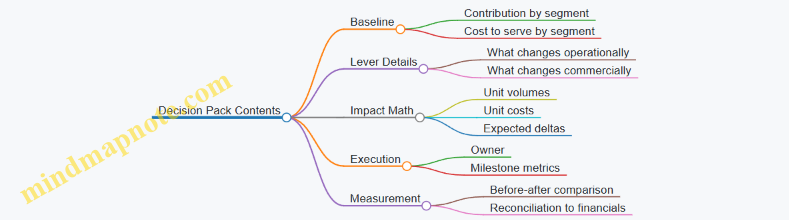
When you do this consistently, prioritization stops being a debate about opinions and becomes a set of calculations tied to operational reality. Contribution tells you where profit is missing; cost to serve tells you what to change; the lever stack tells you what to do first.
12.4 Designing Implementation Tracking with KPI Ownership
Implementation tracking is where good analysis turns into measurable change. The goal is simple: every action has an owner, a KPI target, a measurement method, and a feedback loop that catches issues before month-end surprises.
Step 1: Translate Actions into Measurable Outcomes
Start by converting each recommended action into an outcome statement that can be tested. For example, “Improve pricing discipline” becomes “Increase realized gross margin by reducing unapproved discounting in the top 20% of deals.” Then define the KPI that represents the outcome, not the activity.
Example: If the action is “Standardize freight terms,” the KPI should reflect margin impact (e.g., contribution margin per order after freight), while the activity log records which contracts were updated.
Step 2: Assign KPI Ownership with Clear Boundaries
KPI ownership should match decision authority. A common failure mode is assigning a KPI to someone who can report it but cannot influence it.
Use a three-role split:
- KPI Owner: accountable for target achievement and corrective actions.
- Data Owner: accountable for data quality, definitions, and refresh timing.
- Action Owner: accountable for executing specific initiatives.
Example: A Sales Finance leader may own “realized margin rate,” while Sales Ops owns “discount approval workflow changes,” and Finance Data owns the “deal margin calculation logic.”
Step 3: Define KPI Measurement Rules and Timing
Write down the measurement rules so the KPI is stable across reporting cycles. Include:
- Scope: which products, channels, regions, and customer types.
- Formula: exact inputs and sign conventions.
- Normalization: how you handle returns, rebates, and one-time adjustments.
- Timing: when the KPI is measured (order date vs. invoice date) and when it is reported.
Example: If returns are booked later, decide whether the KPI uses invoice-time margin or net-of-returns margin. Pick one and document it.
Step 4: Build a Tracking Cadence That Matches Decision Speed
Not all KPIs need the same rhythm. Use a cadence matrix:
- Weekly: leading indicators tied to execution (e.g., % deals with approved discounts).
- Monthly: financial KPIs tied to profitability (e.g., contribution margin by segment).
- Quarterly: model health checks and reconciliation status.
Example: If discount approvals are lagging, weekly tracking prevents a month of avoidable margin leakage.
Step 5: Create a KPI-to-Action Map with Evidence Requirements
Every KPI should link to one or more actions. Each action should have evidence that it happened and a mechanism for how it affects the KPI.
Example:
- Action: “Update discount approval thresholds.”
- Evidence: change log, workflow configuration, training completion.
- Mechanism: fewer deals bypass approvals.
- KPI: realized gross margin rate in affected deal bands.
Step 6: Use Variance Logic to Drive Corrective Actions
Tracking should not stop at “we missed the target.” Add variance logic that separates:
- Execution variance: actions not completed or completed late.
- Business variance: market or demand changes.
- Measurement variance: definition or data issues.
Example: If margin drops but approval compliance improved, suspect measurement scope changes or cost-to-serve shifts.
Step 7: Implement a Simple Governance Loop
A lightweight governance loop keeps ownership real:
- RACI for each KPI (who decides, who executes, who provides data).
- Exception thresholds (e.g., if KPI misses by more than 1.0 percentage point for two consecutive weeks).
- Escalation path (who gets pulled in and when).
Example: If “approved discount rate” falls below 95% for two weeks, the KPI owner escalates to Sales Ops to fix workflow friction.
Mind Map: KPI Ownership and Tracking Design
Example: Tracking a Margin Improvement Initiative
Initiative: Reduce unapproved discounting in mid-market deals.
- KPI: realized gross margin rate for mid-market deals.
- KPI Owner: Head of Sales Finance.
- Data Owner: Finance analytics lead.
- Action Owner: Sales Ops manager.
- Leading Indicator (weekly): % deals with approved discounts.
- Measurement Rule: realized gross margin uses invoice margin net of returns booked within the same month; scope excludes strategic contracts.
- Cadence: weekly compliance review; monthly margin review; quarterly reconciliation of deal margin logic to accounting.
- Variance Logic: if compliance improves but margin doesn’t, check cost-to-serve changes and whether discount codes map correctly to margin inputs.
Mind Map: Variance Diagnosis Workflow
Implementation tracking works when it is boring in the best way: consistent definitions, clear ownership, and variance logic that points to a next step rather than a meeting.
12.5 Closing the Loop with Post Review Reconciliations and Learnings
A profitability improvement effort is only as good as what you can explain after the month closes. Closing the loop means you compare what you planned to what actually happened, reconcile differences between analytical and accounting views, and capture learnings in a way that prevents the same confusion from returning next cycle. The goal is not to assign blame; it is to make the next decision easier and the next model more trustworthy.
Post Review Reconciliations
Start with a reconciliation checklist that mirrors how your profit model is built.
- Reconcile revenue and discounts: Confirm that the revenue used in the margin model matches the accounting revenue, then explain differences caused by timing (invoice date vs. shipment date), credit memos, and contract-specific discount recognition.
- Reconcile cost of goods and fulfillment: Verify that direct product costs and fulfillment costs are pulled from the correct ledgers and include the intended accruals. A common issue is missing accruals for freight or returns that hit the next period.
- Reconcile allocations: For activity-based or rule-based allocations, compare total allocated expense to the accounting total for the same period. If totals match but segment results differ, the issue is usually driver mapping or filter logic.
- Reconcile working capital impacts: If your profitability view includes cash conversion assumptions, reconcile them to the actual movement in receivables, inventory, and payables. Even if you do not forecast cash, you should still explain why “profit” and “cash” diverged.
A practical example: suppose a margin waterfall showed a 1.2% gross margin improvement for a customer segment. After reconciliation, you find that accounting gross margin increased by only 0.6%. The remaining 0.6% came from a timing mismatch: the model used shipment date while accounting used invoice date, and a late credit memo landed in the next month.
Learnings Capture That Actually Gets Used
Learnings should be written as decisions and evidence, not as observations. Use a simple template:
- What changed: One sentence describing the driver (e.g., “Discounts increased on expedited orders”).
- Why it happened: The operational or commercial reason (e.g., “Sales approved exceptions without updating deal terms”).
- What the model did: How the model represented it (e.g., “Discounts were treated as revenue reductions, not as separate allowances”).
- What to fix: A specific action (e.g., “Add exception flag to discount feed and re-run allocation”).
- Proof: The reconciliation evidence (e.g., “Credit memo volume explained 0.4% of variance”).
To keep this systematic, assign ownership. Finance owns reconciliation logic; operations owns driver definitions; commercial finance owns deal and discount mapping. If everyone owns it, no one does.
Mind Map: Closing the Loop
Example Workflow for One Month Close
Assume the team ran a profitability improvement initiative in the month ending 2026-03-15. The post review proceeds like this:
- Step 1: Totals check: Accounting gross margin totals match the model within 0.1%. Net income differs by 0.3% due to operating expense allocations.
- Step 2: Segment check: The customer segment that “improved” actually improved in gross margin but not in contribution margin. The gap is traced to higher cost-to-serve from increased returns.
- Step 3: Driver check: Returns were recorded using a different reason code than the one used in the cost-to-serve model. The model treated those returns as normal demand.
- Step 4: Fix and validate: Update the reason code mapping, re-run the month, and confirm that the model now reconciles and the segment story matches the operational reality.
- Step 5: Learning entry: Record that mapping changes must be reviewed during month-end close, not after the next cycle starts.
Common Failure Modes to Prevent
- Reconciling only totals: Totals can match while segment logic is wrong.
- Writing learnings without evidence: “We think it happened” is not a learning; it is a guess.
- Changing the model without re-running: Every change should be validated by re-running the same period and confirming reconciliation.
Closing the loop turns profitability analysis from a one-time report into a repeatable system: reconcile first, diagnose next, and capture learnings as actionable changes tied to proof.